1 brainstorming for presentation of variability in current practices scenario b. contor august 2007
TRANSCRIPT
1
Brainstorming for Presentationof Variability in Current
Practices Scenario
B. Contor
August 2007
2
The first three sections are todescribe the pseudo data.
These will be followed by several sections of possible presentation
formats based upon the pseudo data.
Slides colored yellow are for ESHMC review and not proposed
as alternatives for presentation.
3
Pseudo Data,Monthly Gains Targets
(See spreadsheet “PseudoHistory.xls”)
(Purposely constructed to not look like Snake Plain data, so we don’t get bogged down in
discussions of the data themselves.)
4
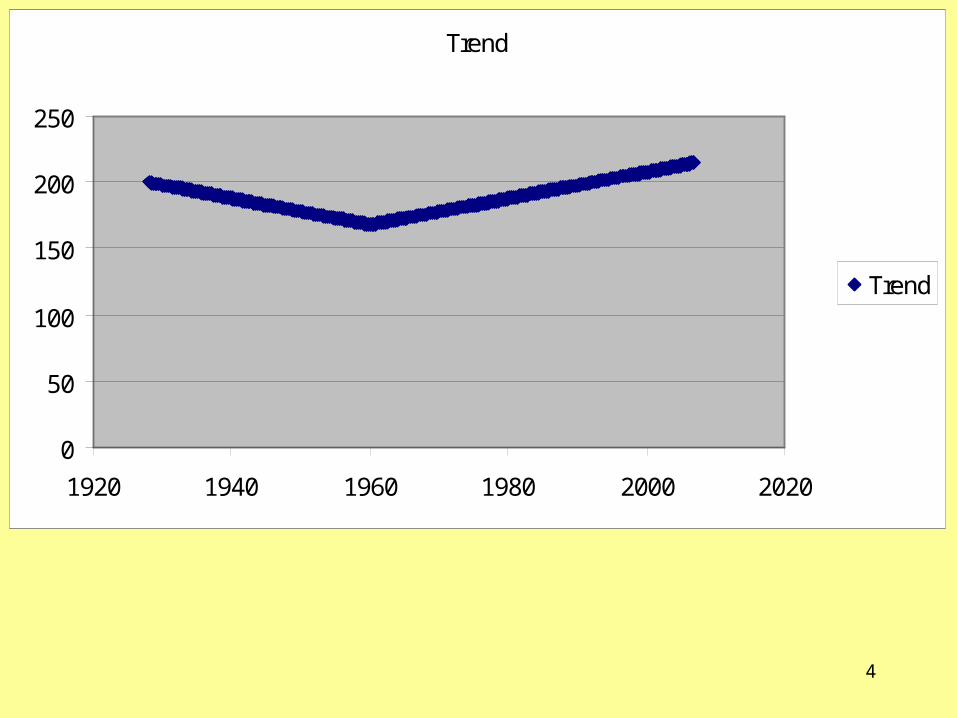
Trend
0
50
100
150
200
250
1920 1940 1960 1980 2000 2020
Trend
5
-2.5
-2
-1.5
-1
-0.5
0
0.5
1
1.5
2
2.5
1920 1940 1960 1980 2000 2020
7-yr Rand
7-yr Sin
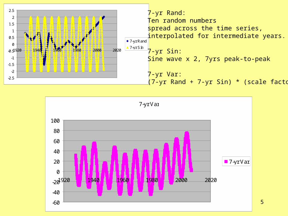
7-yr Rand:Ten random numbersspread across the time series,interpolated for intermediate years.
7-yr Sin:Sine wave x 2, 7yrs peak-to-peak
7-yr Var:(7-yr Rand + 7-yr Sin) * (scale factor)
7-yr Var
-60
-40
-20
0
20
40
60
80
100
1920 1940 1960 1980 2000 2020
7-yr Var
6
3-yr Var
-25
-20
-15
-10
-5
0
5
10
15
20
25
1920 1940 1960 1980 2000 2020
3-yr Var
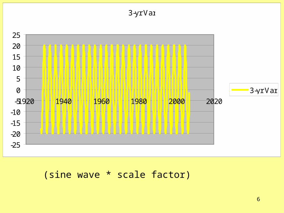
(sine wave * scale factor)
7
Ann Var
-200
-150
-100
-50
0
50
100
150
200
1920 1940 1960 1980 2000 2020
Ann Var
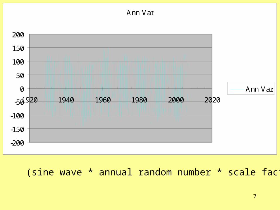
(sine wave * annual random number * scale factor)
8
Rand
-80
-60
-40
-20
0
20
40
60
80
1920 1940 1960 1980 2000 2020
Rand
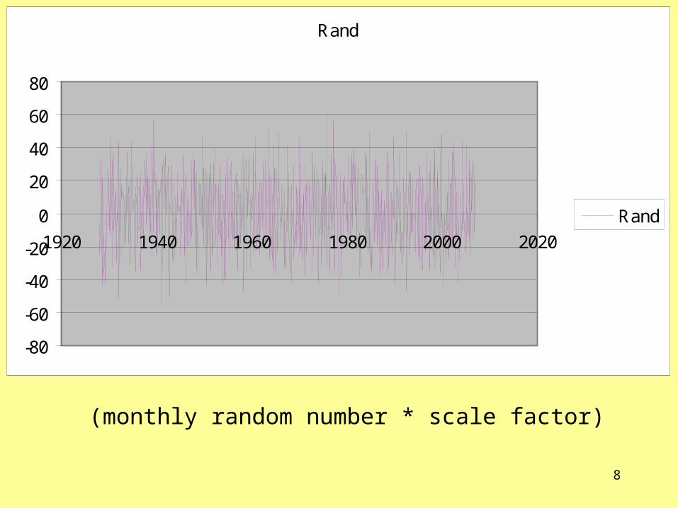
(monthly random number * scale factor)
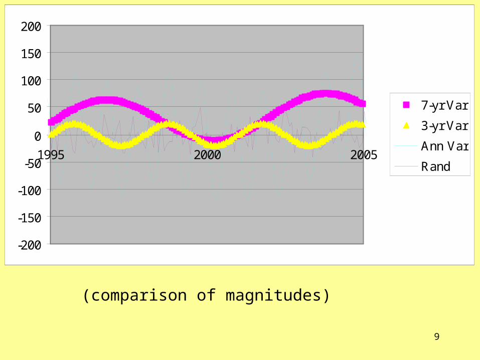
9
-200
-150
-100
-50
0
50
100
150
200
1995 2000 2005
7-yr Var
3-yr Var
Ann Var
Rand
(comparison of magnitudes)
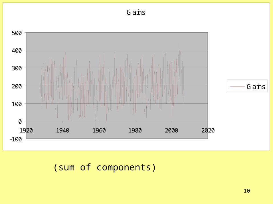
10
Gains
-100
0
100
200
300
400
500
1920 1940 1960 1980 2000 2020
Gains
(sum of components)
11
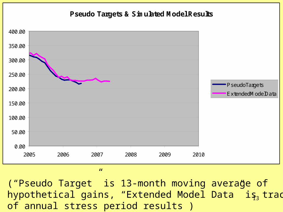
Pseudo Data,Modeling Results,“Extended Data”
(See spreadsheet “PseudoHistory.xls”)
12
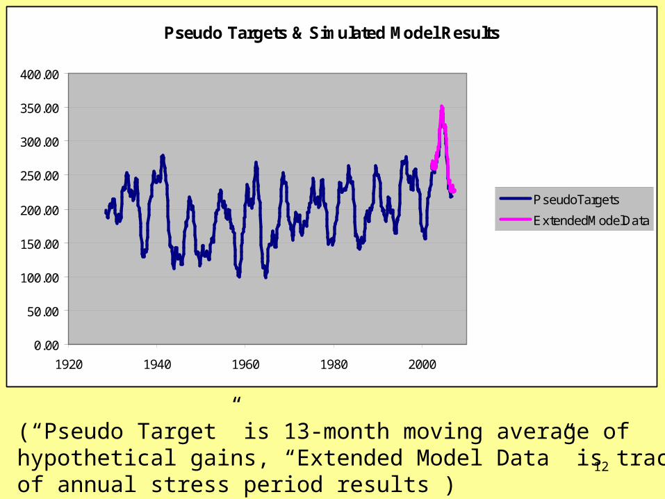
(“Pseudo Target” is 13-month moving average ofhypothetical gains, “Extended Model Data” is traceof annual stress period results )
Pseudo Targets & Simulated Model Results
0.00
50.00
100.00
150.00
200.00
250.00
300.00
350.00
400.00
1920 1940 1960 1980 2000
PseudoTargets
ExtendedModelData
13
Pseudo Targets & Simulated Model Results
0.00
50.00
100.00
150.00
200.00
250.00
300.00
350.00
400.00
2005 2006 2007 2008 2009 2010
PseudoTargets
ExtendedModelData
(“Pseudo Target” is 13-month moving average ofhypothetical gains, “Extended Model Data” is traceof annual stress period results )
14
Pseudo DataModeling Results,“Four Methods”
(See spreadsheet “PseudoHistory.xls”)
15
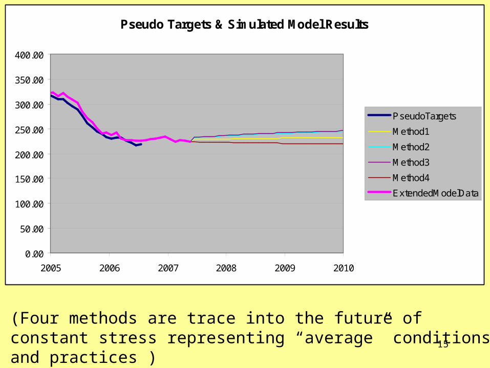
Pseudo Targets & Simulated Model Results
0.00
50.00
100.00
150.00
200.00
250.00
300.00
350.00
400.00
2005 2006 2007 2008 2009 2010
PseudoTargets
Method1
Method2
Method3
Method4
ExtendedModelData
(Four methods are trace into the future ofconstant stress representing “average” conditionsand practices )
16
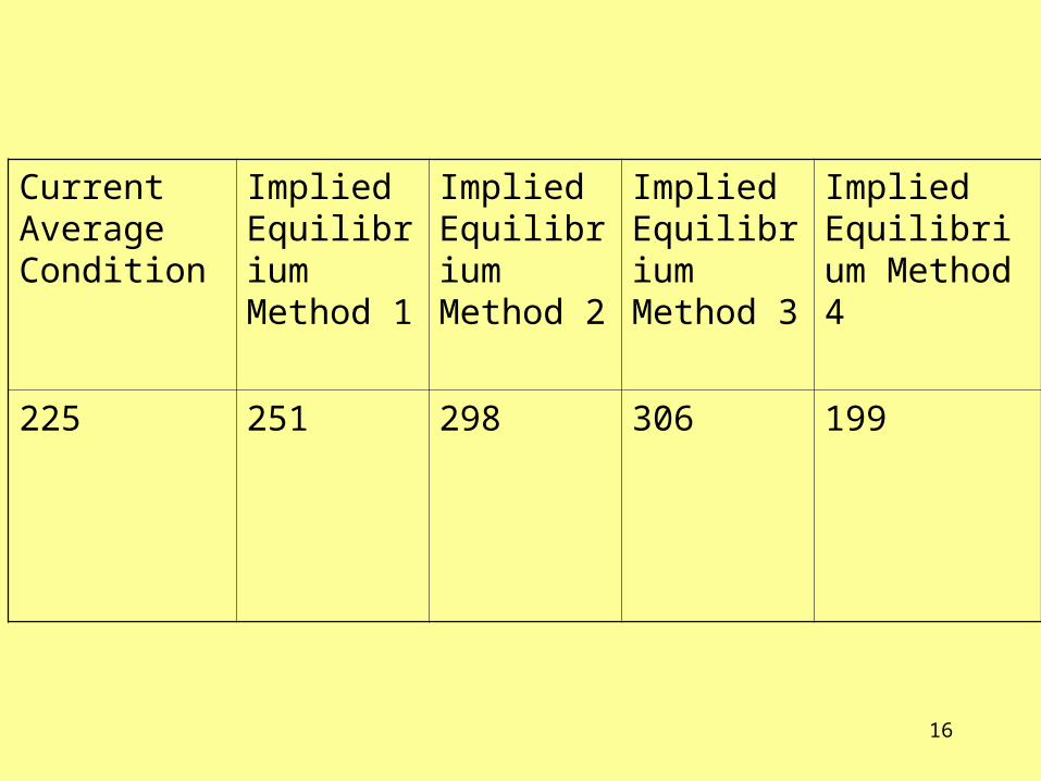
Current Average Condition
Implied Equilibrium Method 1
Implied Equilibrium Method 2
Implied Equilibrium Method 3
Implied Equilibrium Method 4
225 251 298 306 199

17
Presentation of Historical Record, option (a)
18
-100
0
100
200
300
400
500
1920 1940 1960 1980 2000 2020
Gains
Trend
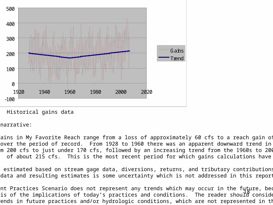
Figure 1: Historical gains data
Proposed narrative:
Monthly gains in My Favorite Reach range from a loss of approximately 60 cfs to a reach gain of over400 cfs, over the period of record. From 1928 to 1960 there was an apparent downward trend in meangains from 200 cfs to just under 170 cfs, followed by an increasing trend from the 1960s to 2006 to a mean gain of about 215 cfs. This is the most recent period for which gains calculations have been completed.
Gains are estimated based on stream gage data, diversions, returns, and tributary contributions. Inherentin these data and resulting estimates is some uncertainty which is not addressed in this report.
The Current Practices Scenario does not represent any trends which may occur in the future, because it is an analysis of the implications of today’s practices and conditions. The reader should consider that theremay be trends in future practices and/or hydrologic conditions, which are not represented in the scenario.
19
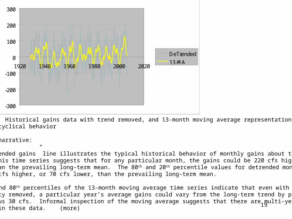
Figure 2: Historical gains data with trend removed, and 13-month moving average representation ofpossible cyclical behavior
Proposed narrative:
The “detrended gains” line illustrates the typical historical behavior of monthly gains about the long-term meanvalue. This time series suggests that for any particular month, the gains could be 220 cfs higher, or 230 cfs lower, than the prevailing long-term mean. The 80 th and 20th percentile values for detrended monthly gains are about 90 cfs higher, or 70 cfs lower, than the prevailing long-term mean.
The 20th and 80th percentiles of the 13-month moving average time series indicate that even with annual variability removed, a particular year’s average gains could vary from the long-term trend by plus50 to minus 30 cfs. Informal inspection of the moving average suggests that there are multi-year cyclicalpatterns in these data. (more)
-300
-200
-100
0
100
200
300
1920 1940 1960 1980 2000 2020
DeTrended
13-MA
20
Proposed narrative for Figure 2 (Continued):
In considering the implications of the Current Practices Scenario, the reader should contemplate boththe historical variability that has been observed in My Favorite Reach as well as the possibility thatfuture changes could occur in both the cyclical and seasonal variability of gains. (If the reach datadid appear to exhibit changes in variability, those would also be pointed out here.)
21
-80
-60
-40
-20
0
20
40
60
80
100
1920 1940 1960 1980 2000 2020
Cyclical
35-MA
Note:
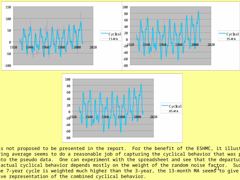
This slide is not proposed to be presented in the report. For the benefit of the ESHMC, it illustrates that the 13-month moving average seems to do a reasonable job of capturing the cyclical behavior that was purposely inserted into the pseudo data. One can experiment with the spreadsheet and see that the departure of the 13-monthMA from the actual cyclical behavior depends mostly on the weight of the random noise factor. Surprisingly, even when the 7-year cycle is weighted much higher than the 3-year, the 13-month MA seems to give the most intuitive representation of the combined cyclical behavior.
-100
-50
0
50
100
150
1920 1940 1960 1980 2000 2020
Cyclical
13-MA
-80
-60
-40
-20
0
20
40
60
80
100
1920 1940 1960 1980 2000 2020
Cyclical
85-MA

22
Presentation of Historical Record, option (b)
23
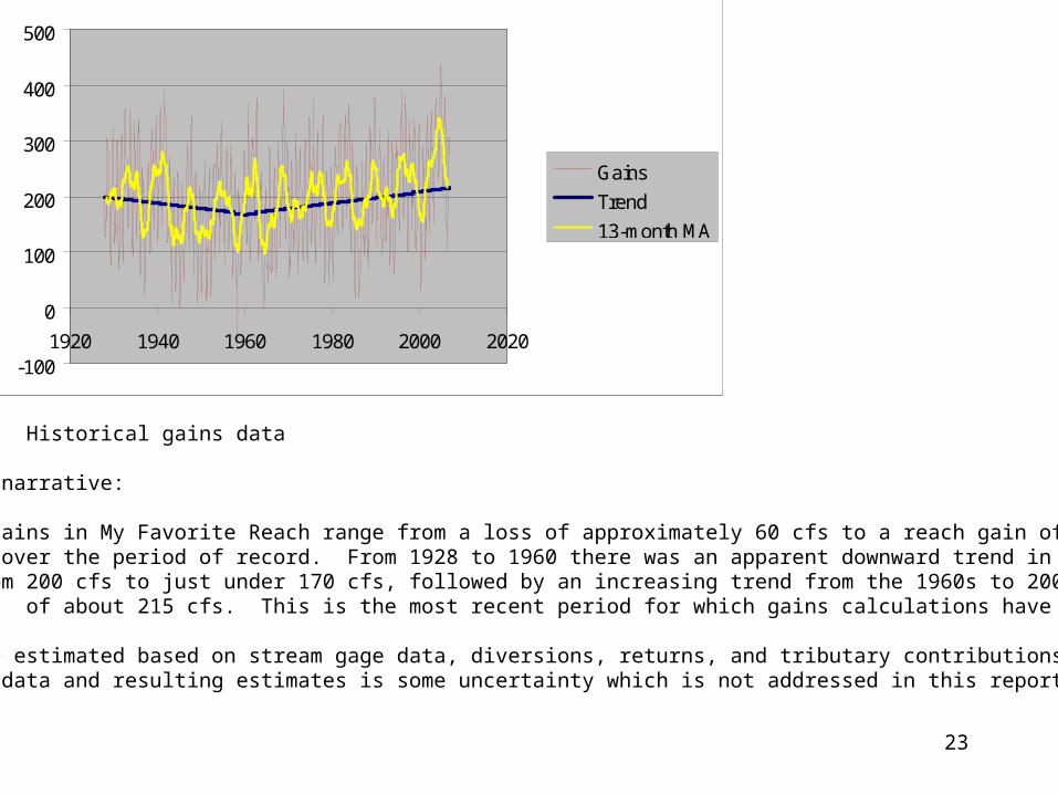
Figure 1: Historical gains data
Proposed narrative:
Monthly gains in My Favorite Reach range from a loss of approximately 60 cfs to a reach gain of over400 cfs, over the period of record. From 1928 to 1960 there was an apparent downward trend in meangains from 200 cfs to just under 170 cfs, followed by an increasing trend from the 1960s to 2006 to a mean gain of about 215 cfs. This is the most recent period for which gains calculations have been completed.
Gains are estimated based on stream gage data, diversions, returns, and tributary contributions. Inherentin these data and resulting estimates is some uncertainty which is not addressed in this report.
(more)
-100
0
100
200
300
400
500
1920 1940 1960 1980 2000 2020
Gains
Trend
13-month MA
24
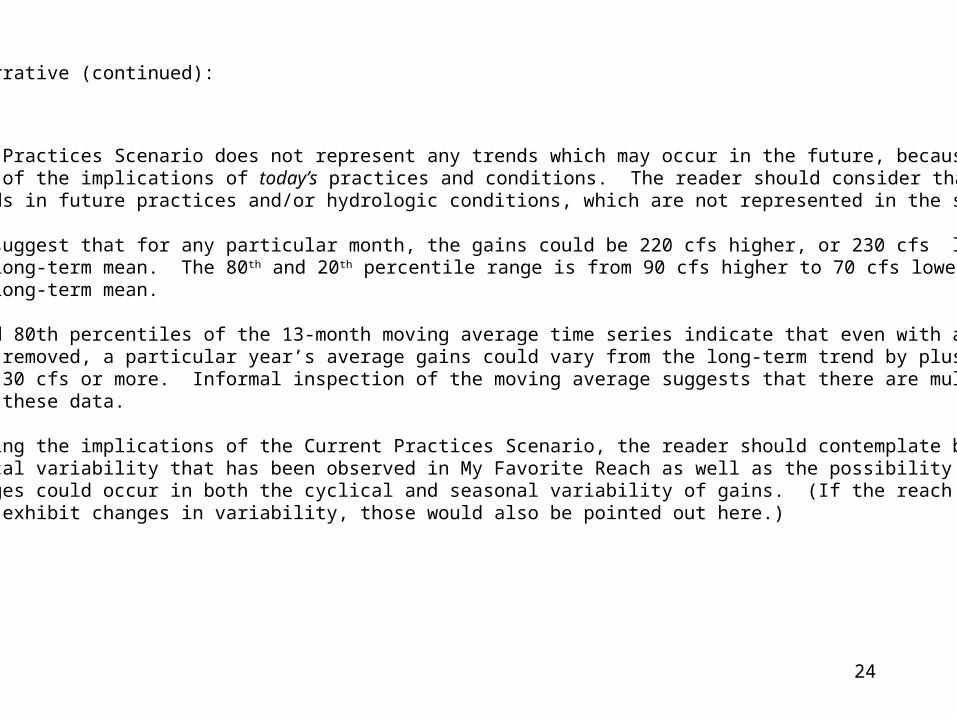
Proposed narrative (continued):
The Current Practices Scenario does not represent any trends which may occur in the future, because it is an analysis of the implications of today’s practices and conditions. The reader should consider that theremay be trends in future practices and/or hydrologic conditions, which are not represented in the scenario.
These data suggest that for any particular month, the gains could be 220 cfs higher, or 230 cfs lower, than the prevailing long-term mean. The 80th and 20th percentile range is from 90 cfs higher to 70 cfs lower than the prevailing long-term mean.
The 20th and 80th percentiles of the 13-month moving average time series indicate that even with annual variability removed, a particular year’s average gains could vary from the long-term trend by plus50 to minus 30 cfs or more. Informal inspection of the moving average suggests that there are multi-year cyclicalpatterns in these data.
In considering the implications of the Current Practices Scenario, the reader should contemplate boththe historical variability that has been observed in My Favorite Reach as well as the possibility thatfuture changes could occur in both the cyclical and seasonal variability of gains. (If the reach dataappeared to exhibit changes in variability, those would also be pointed out here.)

25
Presentation of Historical Record, option (c)
26
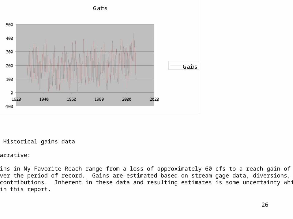
Figure 1: Historical gains data
Proposed narrative:
Monthly gains in My Favorite Reach range from a loss of approximately 60 cfs to a reach gain of over400 cfs, over the period of record. Gains are estimated based on stream gage data, diversions, returns, and tributary contributions. Inherent in these data and resulting estimates is some uncertainty which is not addressed in this report.
(more)
Gains
-100
0
100
200
300
400
500
1920 1940 1960 1980 2000 2020
Gains
27
Proposed narrative (continued):
Inspection of these data suggests that reach gains are subject to annual variability, short- to medium-termcyclical variability, and to longer-term trends. The Current Practices Scenario does not represent any trendsor cyclical variability, because the purpose is to estimate the average equilibrium implied bycurrent practices and conditions. In interpreting scenario results, the reader should contemplate the futuretrends and variability that may be expected to occur. The reader should also consider that a consequenceof changing conditions and practices may be that future trends and variability patterns will not be identicalto the trends and patterns observed in the past.
28
Presentation of AlternateScenario Simulations, option (1)
29
Average Reach Gains, My Favorite Reach
-100
0
100
200
300
400
500
600
2000 2002 2004 2006 2008 2010
Year
cfs
Method1 Method2 Method3
Method4 Max Min
80th 20th ExtendedModelData
PseudoTargets
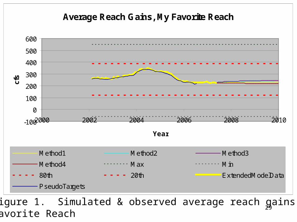
Figure 1. Simulated & observed average reach gains for MyFavorite Reach
30
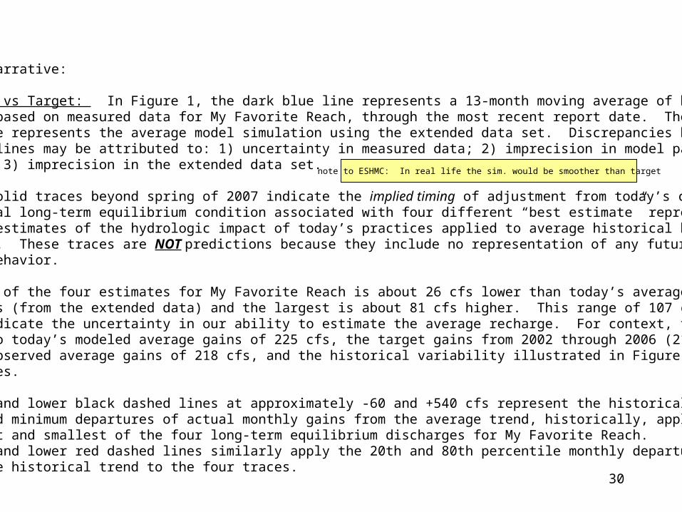
Proposed narrative:
Simulation vs Target: In Figure 1, the dark blue line represents a 13-month moving average of historical gainsestimates based on measured data for My Favorite Reach, through the most recent report date. The heavy yellow line represents the average model simulation using the extended data set. Discrepancies betweenthese two lines may be attributed to: 1) uncertainty in measured data; 2) imprecision in model parametersand setup; 3) imprecision in the extended data set.
The four solid traces beyond spring of 2007 indicate the implied timing of adjustment from today’s condition to thehypothetical long-term equilibrium condition associated with four different “best estimate” representations.These are estimates of the hydrologic impact of today’s practices applied to average historical hydrologic conditions. These traces are NOT predictions because they include no representation of any future trends or cyclical behavior.
The lowest of the four estimates for My Favorite Reach is about 26 cfs lower than today’s average modeledreach gains (from the extended data) and the largest is about 81 cfs higher. This range of 107 cfs from lowto high indicate the uncertainty in our ability to estimate the average recharge. For context, this range may be compared to today’s modeled average gains of 225 cfs, the target gains from 2002 through 2006 (217 to 315cfs), the 2006 observed average gains of 218 cfs, and the historical variability illustrated in Figure 1 with the dashed lines.
The upper and lower black dashed lines at approximately -60 and +540 cfs represent the historicalmaximum and minimum departures of actual monthly gains from the average trend, historically, applied to the largest and smallest of the four long-term equilibrium discharges for My Favorite Reach. The upper and lower red dashed lines similarly apply the 20th and 80th percentile monthly departures fromthe average historical trend to the four traces.
note to ESHMC: In real life the sim. would be smoother than target
31
Presentation of AlternateScenario Simulations, option (2)
(this option would essentiallybe the format in the
slides presented to ESHMC23 July 2007, which included blue
vertical error bars added tothe upper and lower traces)
32
Presentation of AlternateScenario Simulations, option (3)
33
Average Reach Gains, My Favorite Reach
150
200
250
300
350
400
2000 2002 2004 2006 2008 2010
Year
cfs
Method1 Method2 Method3
Method4 MaxEq MinEq
ExtendedModelData PseudoTargets
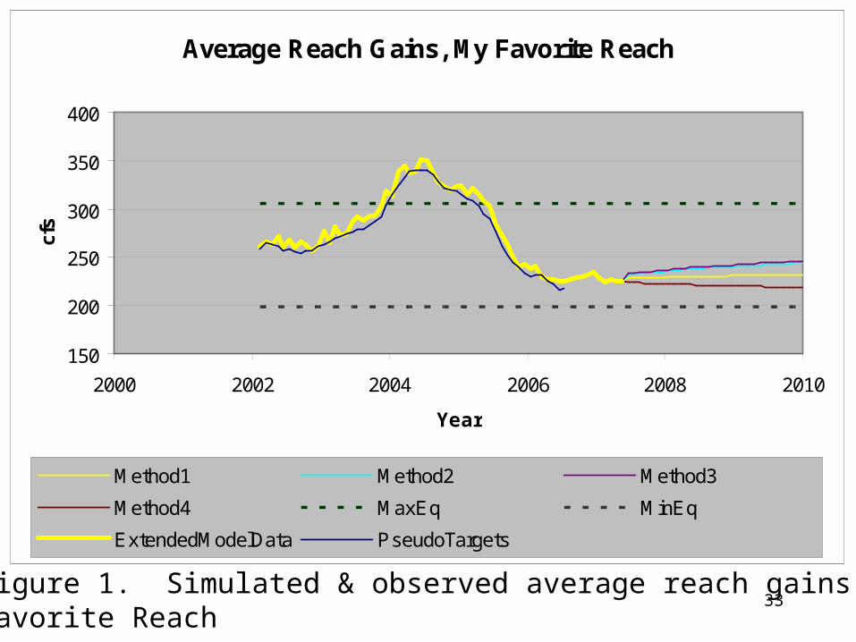
Figure 1. Simulated & observed average reach gains for MyFavorite Reach
34
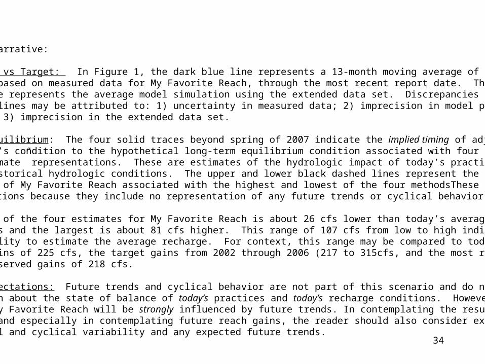
Proposed narrative:
Simulation vs Target: In Figure 1, the dark blue line represents a 13-month moving average of historical gainsestimates based on measured data for My Favorite Reach, through the most recent report date. The heavy yellow line represents the average model simulation using the extended data set. Discrepancies betweenthese two lines may be attributed to: 1) uncertainty in measured data; 2) imprecision in model parametersand setup; 3) imprecision in the extended data set.
Implied Equilibrium: The four solid traces beyond spring of 2007 indicate the implied timing of adjustment from today’s condition to the hypothetical long-term equilibrium condition associated with four different “best estimate” representations. These are estimates of the hydrologic impact of today’s practices applied toaverage historical hydrologic conditions. The upper and lower black dashed lines represent the final equilibrium discharges of My Favorite Reach associated with the highest and lowest of the four methodsThese traces are NOT predictions because they include no representation of any future trends or cyclical behavior.
The lowest of the four estimates for My Favorite Reach is about 26 cfs lower than today’s average modeledreach gains and the largest is about 81 cfs higher. This range of 107 cfs from low to high indicates uncertaintyin our ability to estimate the average recharge. For context, this range may be compared to today’s modeled average gains of 225 cfs, the target gains from 2002 through 2006 (217 to 315cfs, and the most recent (2006)average observed gains of 218 cfs.
Future Expectations: Future trends and cyclical behavior are not part of this scenario and do not communicate information about the state of balance of today’s practices and today’s recharge conditions. However, actual futuregains in My Favorite Reach will be strongly influenced by future trends. In contemplating the results of thisscenario, and especially in contemplating future reach gains, the reader should also consider expectationsof seasonal and cyclical variability and any expected future trends.

35
Presentation of AlternateScenario Simulations, option (4)
36
Average Reach Gains, My Favorite Reach
150
200
250
300
350
400
2000 2002 2004 2006 2008 2010
Year
cfs
Method1 Method2 Method3
Method4 ExtendedModelData PseudoTargets
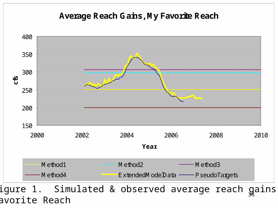
Figure 1. Simulated & observed average reach gains for MyFavorite Reach
37
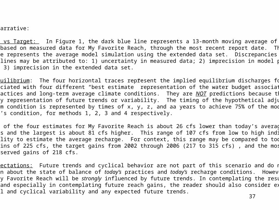
Proposed narrative:
Simulation vs Target: In Figure 1, the dark blue line represents a 13-month moving average of historical gainsestimates based on measured data for My Favorite Reach, through the most recent report date. The heavy yellow line represents the average model simulation using the extended data set. Discrepancies betweenthese two lines may be attributed to: 1) uncertainty in measured data; 2) imprecision in model parametersand setup; 3) imprecision in the extended data set.
Implied Equilibrium: The four horizontal traces represent the implied equilibrium discharges for My FavoriteReach associated with four different “best estimate” representation of the water budget associated withtoday’s practices and long-term average climate conditions. They are NOT predictions because they do notinclude any representation of future trends or variability. The timing of the hypothetical adjustment to thisequilibrium condition is represented by times of x, y, z, and aa years to achieve 75% of the modeled changefrom today’s condition, for methods 1, 2, 3 and 4 respectively.
The lowest of the four estimates for My Favorite Reach is about 26 cfs lower than today’s average modeledreach gains and the largest is about 81 cfs higher. This range of 107 cfs from low to high indicates uncertaintyin our ability to estimate the average recharge. For context, this range may be compared to today’s modeled average gains of 225 cfs, the target gains from 2002 through 2006 (217 to 315 cfs) , and the most recent (2006)average observed gains of 218 cfs.
Future Expectations: Future trends and cyclical behavior are not part of this scenario and do not communicate information about the state of balance of today’s practices and today’s recharge conditions. However, actual futuregains in My Favorite Reach will be strongly influenced by future trends. In contemplating the results of thisscenario, and especially in contemplating future reach gains, the reader should also consider expectationsof seasonal and cyclical variability and any expected future trends.

38
Presentation of AlternateScenario Simulations, option (5)
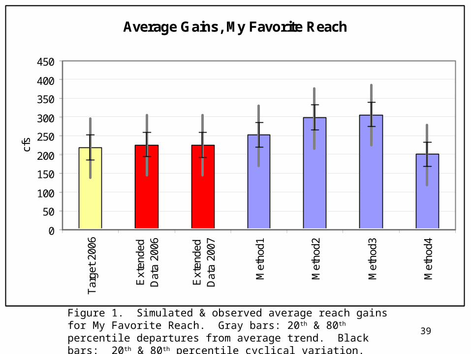
39
Figure 1. Simulated & observed average reach gains for My Favorite Reach. Gray bars: 20th & 80th percentile departures from average trend. Black bars: 20th & 80th percentile cyclical variation.
Average Gains, My Favorite Reach
0
50
100
150
200
250
300
350
400
450
Tar
get
2006
Ext
ende
dD
ata
2006
Ext
ende
dD
ata
2007
Met
hod1
Met
hod2
Met
hod3
Met
hod4
cfs
Average Gains, My Favorite Reach
0
50
100
150
200
250
300
350
400
450
Tar
get
2006
Ext
ende
dD
ata
2006
Ext
ende
dD
ata
2007
Met
hod1
Met
hod2
Met
hod3
Met
hod4
cfs
40
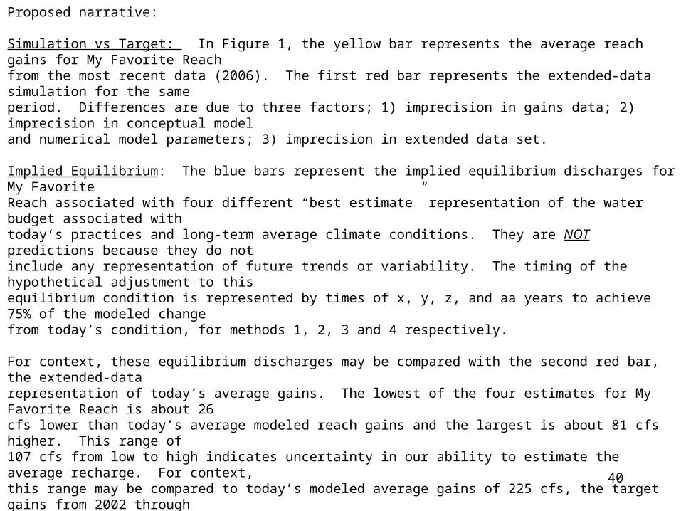
Proposed narrative:
Simulation vs Target: In Figure 1, the yellow bar represents the average reach gains for My Favorite Reachfrom the most recent data (2006). The first red bar represents the extended-data simulation for the sameperiod. Differences are due to three factors; 1) imprecision in gains data; 2) imprecision in conceptual modeland numerical model parameters; 3) imprecision in extended data set.
Implied Equilibrium: The blue bars represent the implied equilibrium discharges for My FavoriteReach associated with four different “best estimate” representation of the water budget associated withtoday’s practices and long-term average climate conditions. They are NOT predictions because they do notinclude any representation of future trends or variability. The timing of the hypothetical adjustment to thisequilibrium condition is represented by times of x, y, z, and aa years to achieve 75% of the modeled changefrom today’s condition, for methods 1, 2, 3 and 4 respectively.
For context, these equilibrium discharges may be compared with the second red bar, the extended-data representation of today’s average gains. The lowest of the four estimates for My Favorite Reach is about 26cfs lower than today’s average modeled reach gains and the largest is about 81 cfs higher. This range of 107 cfs from low to high indicates uncertainty in our ability to estimate the average recharge. For context,this range may be compared to today’s modeled average gains of 225 cfs, the target gains from 2002 through 2006 (217 to 315 cfs) , and the most recent (2006) average observed gains of 218 cfs.
(more)
41
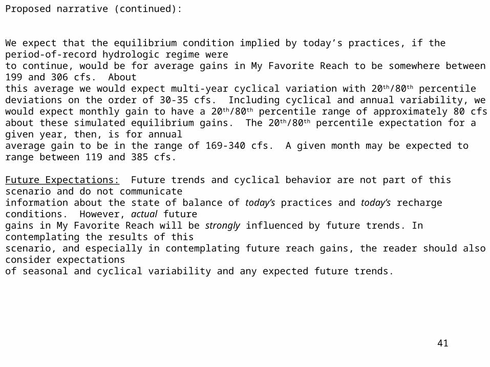
Proposed narrative (continued):
We expect that the equilibrium condition implied by today’s practices, if the period-of-record hydrologic regime wereto continue, would be for average gains in My Favorite Reach to be somewhere between 199 and 306 cfs. Aboutthis average we would expect multi-year cyclical variation with 20 th/80th percentile deviations on the order of 30-35 cfs. Including cyclical and annual variability, we would expect monthly gain to have a 20 th/80th percentile range of approximately 80 cfs about these simulated equilibrium gains. The 20 th/80th percentile expectation for a given year, then, is for annualaverage gain to be in the range of 169-340 cfs. A given month may be expected to range between 119 and 385 cfs.
Future Expectations: Future trends and cyclical behavior are not part of this scenario and do not communicate information about the state of balance of today’s practices and today’s recharge conditions. However, actual futuregains in My Favorite Reach will be strongly influenced by future trends. In contemplating the results of thisscenario, and especially in contemplating future reach gains, the reader should also consider expectationsof seasonal and cyclical variability and any expected future trends.