1

Chapter 12

Inference About One Inference About One PopulationPopulation

Inference About One Inference About One PopulationPopulation

2

12.1 Introduction12.1 Introduction

• In this chapter we utilize the approach In this chapter we utilize the approach developed before to describe a population.developed before to describe a population.– Identify the parameter to be estimated or tested.Identify the parameter to be estimated or tested.– Specify the parameter’s estimator and its sampling Specify the parameter’s estimator and its sampling

distribution.distribution.– Construct a confidence interval estimator or perform Construct a confidence interval estimator or perform

a hypothesis test.a hypothesis test.

3

• We shall develop techniques to estimate and test three population parameters.– Population mean – Population variance 2

– Population proportion p

12.1 Introduction12.1 Introduction

4

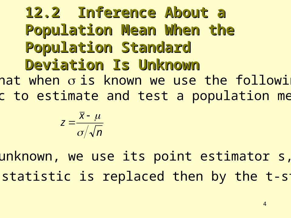
Recall that when is known we use the following statistic to estimate and test a population mean

When is unknown, we use its point estimator s,

and the z-statistic is replaced then by the t-statistic

12.2 Inference About a Population Mean 12.2 Inference About a Population Mean When the Population Standard Deviation When the Population Standard Deviation Is UnknownIs Unknown

n

xz

5

The t - StatisticThe t - Statistic

n

x

n

x

sn

x

Z t

s ss s

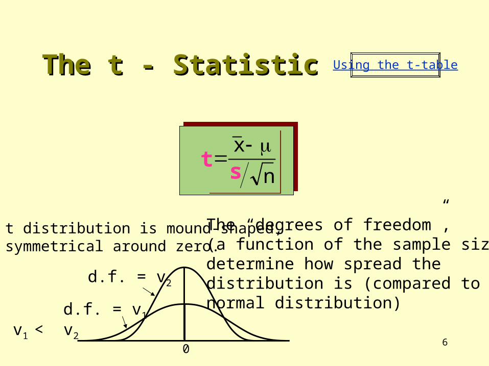
When the sampled population is normally distributed,the t statistic is Student t distributed.

ZZZZZt t t t t t t t t

sss s s

t

6

The t - StatisticThe t - Statistic

n

x

n

x

s

0

The t distribution is mound-shaped, and symmetrical around zero.

The “degrees of freedom”,(a function of the sample size)determine how spread thedistribution is (compared to the normal distribution)

d.f. = v2

d.f. = v1

v1 < v2

t

Using the t-table

7

Testing Testing when when is unknown is unknown

• Example 12.1 - Productivity of newly hired Trainees

8

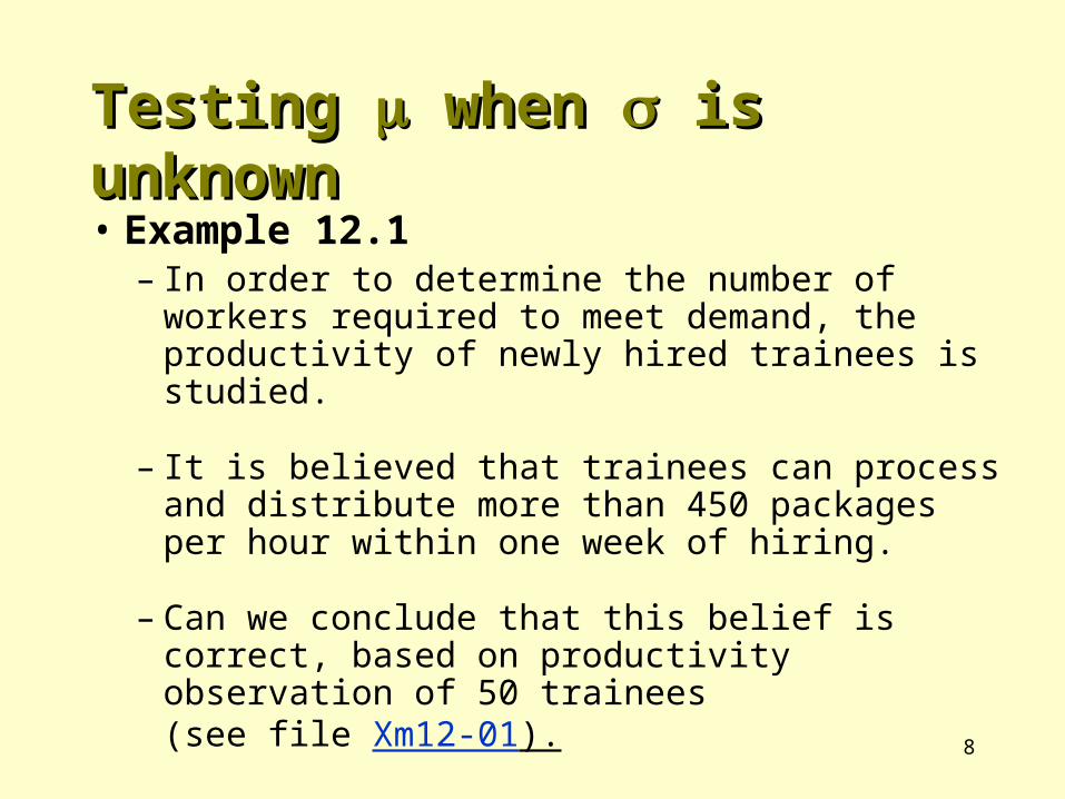
• Example 12.1– In order to determine the number of workers required

to meet demand, the productivity of newly hired trainees is studied.

– It is believed that trainees can process and distribute more than 450 packages per hour within one week of hiring.

– Can we conclude that this belief is correct, based on productivity observation of 50 trainees (see file Xm12-01).

Testing Testing when when is unknown is unknown

9

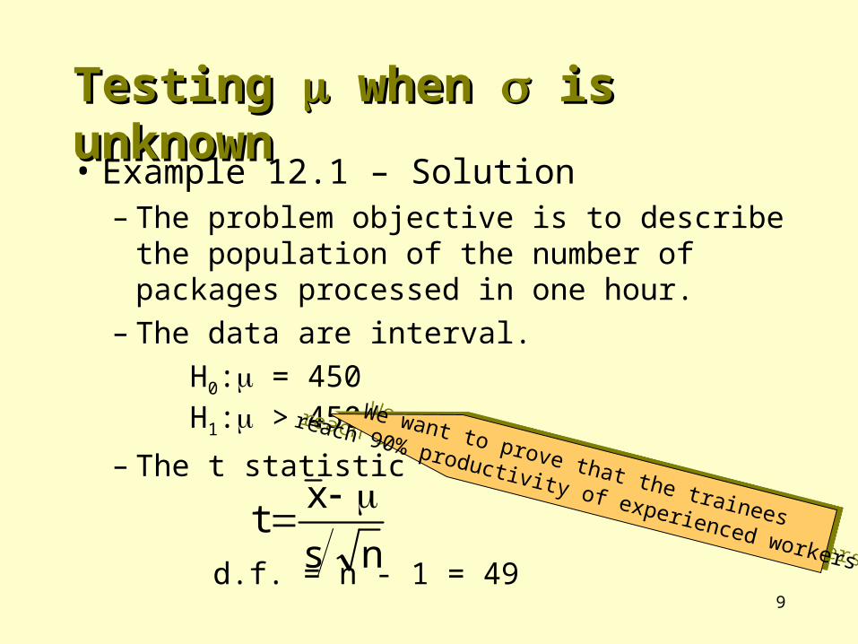
• Example 12.1 – Solution– The problem objective is to describe the population

of the number of packages processed in one hour.– The data are interval.

H0: = 450 H1: > 450

– The t statistic

d.f. = n - 1 = 49ns

xt

We want to prove that the trainees

reach 90% productivity of experienced workers

We want to prove that the trainees

reach 90% productivity of experienced workers

Testing Testing when when is unknown is unknown

10

• Solution continued (solving by hand) – The rejection region is

t > t,n – 1

t,n - 1 = t.05,49

t.05,50 = 1.676.

83.3855.1507s

.55.15071n

nx

xs

and,38.46050019,23

x

thus,357,671,10x019,23x

havewedatatheFrom

2

i2i2

2ii

Testing Testing when when is unknown is unknown

11

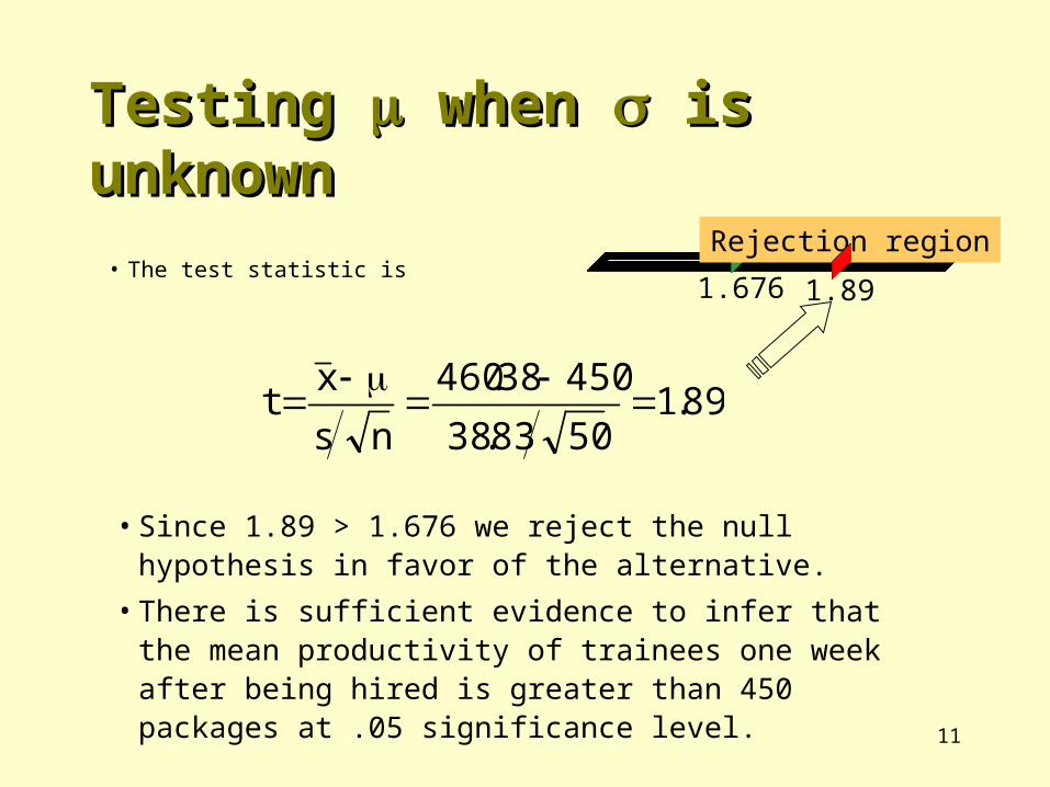
• The test statistic is

89.15083.38

45038.460

ns

xt

• Since 1.89 > 1.676 we reject the null hypothesis in favor of the alternative.

• There is sufficient evidence to infer that the mean productivity of trainees one week after being hired is greater than 450 packages at .05 significance level.

1.676 1.89

Rejection region

Testing Testing when when is unknown is unknown

12

Testing Testing when when is unknown is unknown

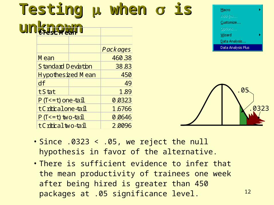
• Since .0323 < .05, we reject the null hypothesis in favor of the alternative.

• There is sufficient evidence to infer that the mean productivity of trainees one week after being hired is greater than 450 packages at .05 significance level.

.05

.0323

t-Test: Mean

PackagesMean 460.38Standard Deviation 38.83Hypothesized Mean 450df 49t Stat 1.89P(T<=t) one-tail 0.0323t Critical one-tail 1.6766P(T<=t) two-tail 0.0646t Critical two-tail 2.0096

13

Estimating Estimating when when is unknown is unknown

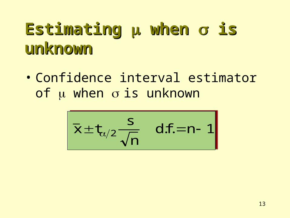
• Confidence interval estimator of when is unknown

1n.f.dn

stx 2 1n.f.d

n

stx 2

14

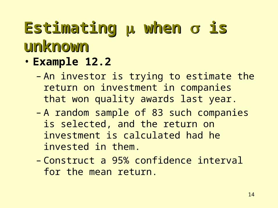
• Example 12.2– An investor is trying to estimate the return on

investment in companies that won quality awards last year.

– A random sample of 83 such companies is selected, and the return on investment is calculated had he invested in them.

– Construct a 95% confidence interval for the mean return.

Estimating Estimating when when is unknown is unknown

15

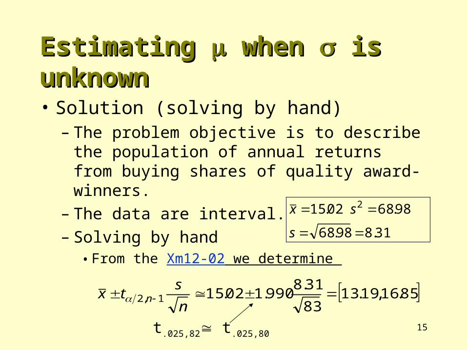
• Solution (solving by hand)– The problem objective is to describe the population

of annual returns from buying shares of quality award-winners.

– The data are interval.– Solving by hand

• From the Xm12-02 we determine

31.898.68

98.6802.15 2

s

sx

85.16,19.1383

31.8990.102.151,2

n

stx n

t.025,82 t.025,80

Estimating Estimating when when is unknown is unknown

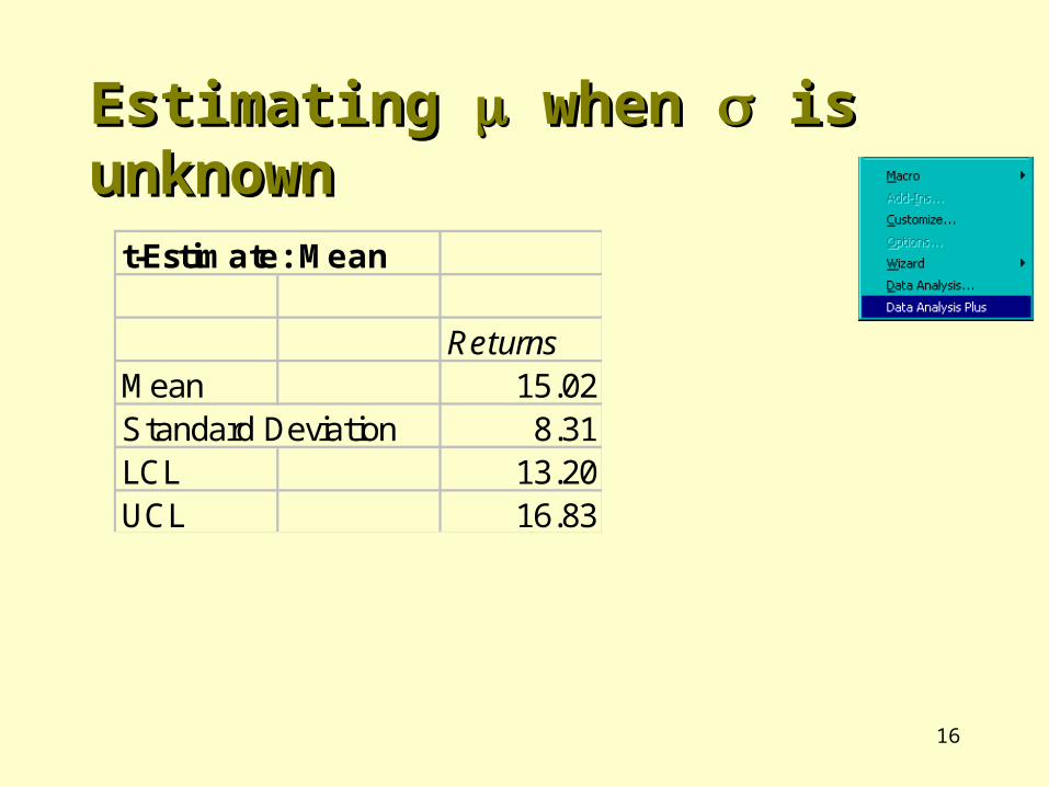
16

Estimating Estimating when when is unknown is unknown

t-Estimate: Mean

ReturnsMean 15.02Standard Deviation 8.31LCL 13.20UCL 16.83

17

Checking the required conditionsChecking the required conditions

• We need to check that the population is normally distributed, or at least not extremely nonnormal.

• There are statistical methods to test for normality (one to be introduced later in the book).

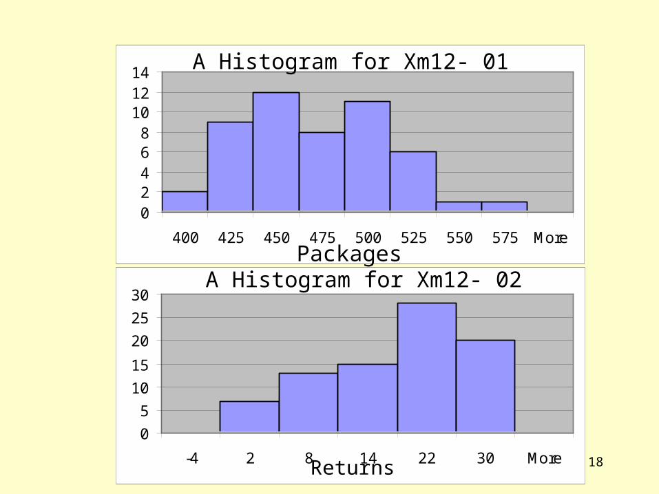
• From the sample histograms we see…

18

0

5

10

15

20

25

30

-4 2 8 14 22 30 More

02468

101214

400 425 450 475 500 525 550 575 More

A Histogram for Xm12- 01

PackagesA Histogram for Xm12- 02

Returns

19

12.3 Inference About a Population Variance12.3 Inference About a Population Variance

• Sometimes we are interested in making inference about the variability of processes.

• Examples:– The consistency of a production process for quality

control purposes.– Investors use variance as a measure of risk.

• To draw inference about variability, the parameter of interest is 2.

20

• The sample variance s2 is an unbiased, consistent and efficient point estimator for 2.

• The statistic has a distribution called Chi-squared, if the population is normally distributed.

2

2s)1n(

1n.f.ds)1n(

2

22

1n.f.ds)1n(

2

22

d.f. = 5

d.f. = 10

12.3 Inference About a Population Variance12.3 Inference About a Population Variance

21

Testing and Estimating a Population Testing and Estimating a Population VarianceVariance

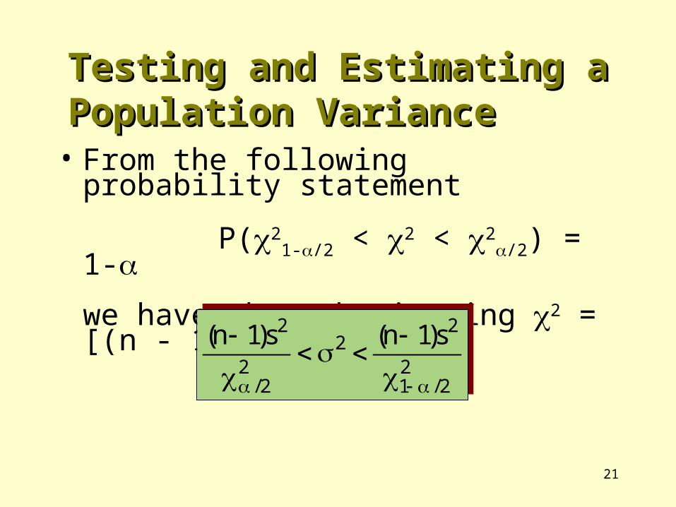
• From the following probability statement

P(21-/2 < 2 < 2

/2) = 1-

we have (by substituting 2 = [(n - 1)s2]/2.)

22/1

22

22/

2 s)1n(s)1n(

22/1

22

22/

2 s)1n(s)1n(

22

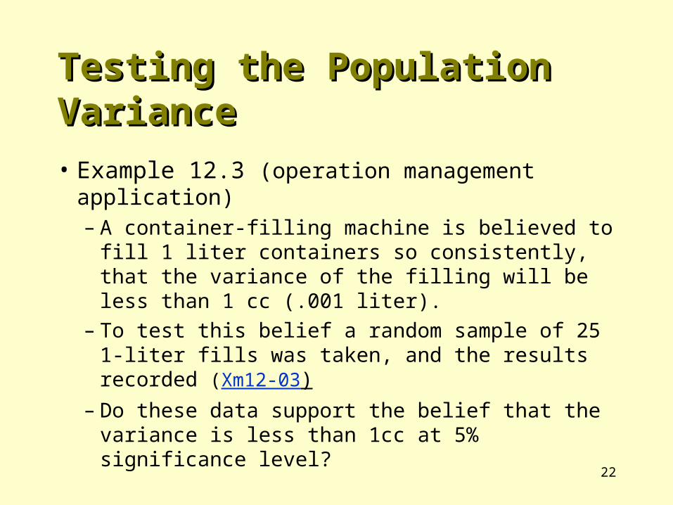
• Example 12.3 (operation management application)– A container-filling machine is believed to fill 1 liter

containers so consistently, that the variance of the filling will be less than 1 cc (.001 liter).

– To test this belief a random sample of 25 1-liter fills was taken, and the results recorded (Xm12-03)

– Do these data support the belief that the variance is less than 1cc at 5% significance level?

Testing the Population VarianceTesting the Population Variance

23

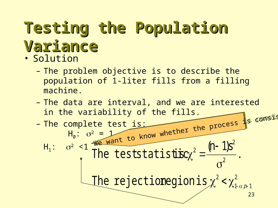
• Solution– The problem objective is to describe the population of 1-liter fills

from a filling machine. – The data are interval, and we are interested in the variability of

the fills.– The complete test is:

H0: 2 = 1

H1: 2 <1

21n,1

2

2

22

isregionrejectionThe

.s)1n(

isstatistictestThe

We want to know whether the process is consistent

We want to know whether the process is consistent

Testing the Population VarianceTesting the Population Variance

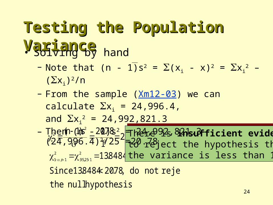
24.hypothesisnullthe

rejectnotdo,78.208484.13Since

.8484.13

,78.201

78.20s)1n(

2

125,95.

2

1n,1

22

22

There is insufficient evidence to reject the hypothesis thatthe variance is less than 1.

There is insufficient evidence to reject the hypothesis thatthe variance is less than 1.

• Solving by hand– Note that (n - 1)s2 = (xi - x)2 = xi

2 – (xi)2/n – From the sample (Xm12-03) we can calculate xi = 24,996.4,

and xi2 = 24,992,821.3

– Then (n - 1)s2 = 24,992,821.3-(24,996.4)2/25 =20.78

Testing the Population VarianceTesting the Population Variance

25

13.8484 20.8

Rejectionregion

8484.132 2

2125,95.

= .05 1- = .95

Do not reject the null hypothesis

Testing the Population VarianceTesting the Population Variance

26

Estimating the Population VarianceEstimating the Population Variance

• Example 12.4– Estimate the variance of fills in Example 12.3 with

99% confidence.• Solution

– We have (n-1)s2 = 20.78.From the Chi-squared table we have2

/2,n-1 = 2.005, 24 = 45.5585

2/2,n-1 2

.995, 24 = 9.88623

27

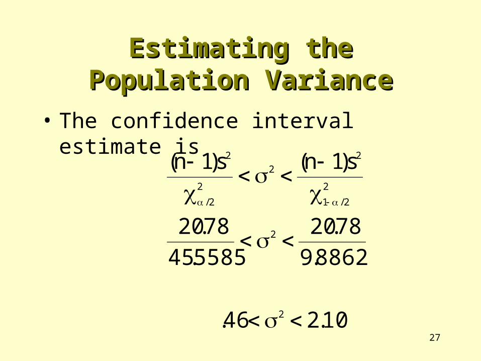
• The confidence interval estimate is

10.246.

88623.978.20

5585.4578.20

s)1n(s)1n(

2

2

2

2/1

22

2

2/

2

Estimating the Population VarianceEstimating the Population Variance

28

12.4 Inference About a Population 12.4 Inference About a Population ProportionProportion

• When the population consists of nominal data, the only inference we can make is about the proportion of occurrence of a certain value.

• The parameter p was used before to calculate these probabilities under the binomial distribution.

29

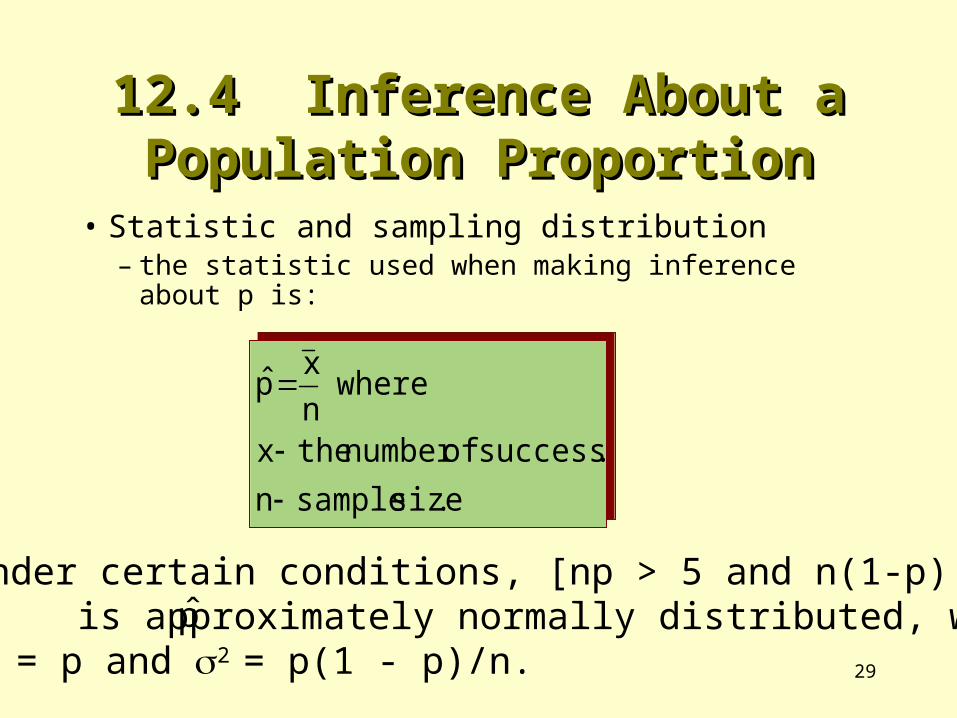
.sizesamplen.successesofnumberthex

wherenx

p̂

.sizesamplen.successesofnumberthex

wherenx

p̂

• Statistic and sampling distribution– the statistic used when making inference about p is:

– Under certain conditions, [np > 5 and n(1-p) > 5], is approximately normally distributed, with

= p and 2 = p(1 - p)/n.p̂

12.4 Inference About a Population 12.4 Inference About a Population ProportionProportion

30

Testing and Estimating the ProportionTesting and Estimating the Proportion

• Test statistic for p

• Interval estimator for p (1- confidence level)

5)p1(nand5npwhere

n/)p1(ppp̂

Z

5)p1(nand5npwhere

n/)p1(ppp̂

Z

5)p̂1(nand5p̂nprovided

n/)p̂1(p̂zp̂ 2/

5)p̂1(nand5p̂nprovided

n/)p̂1(p̂zp̂ 2/

31

• Example 12.5 (Predicting the winner in election day)– Voters are asked by a certain network to participate in an

exit poll in order to predict the winner on election day.– Based on the data presented in Xm12-05 where

1=Democrat, and 2=Republican), can the network conclude that the republican candidate will win the state college vote?

Testing the ProportionTesting the Proportion

Additional example

32

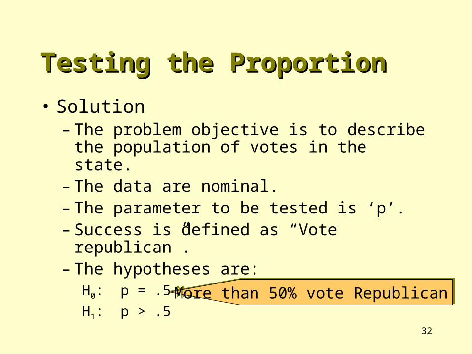
• Solution– The problem objective is to describe the population

of votes in the state.– The data are nominal.– The parameter to be tested is ‘p’.– Success is defined as “Vote republican”.– The hypotheses are:

H0: p = .5H1: p > .5 More than 50% vote RepublicanMore than 50% vote Republican

Testing the ProportionTesting the Proportion

33

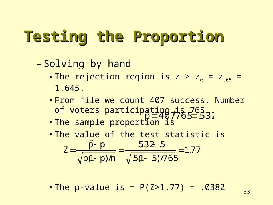
– Solving by hand• The rejection region is z > z = z.05 = 1.645.• From file we count 407 success. Number of voters

participating is 765.• The sample proportion is• The value of the test statistic is

• The p-value is = P(Z>1.77) = .0382

532.765407p̂

77.1765/)5.1(5.

5.532.

n/)p1(p

pp̂Z

Testing the ProportionTesting the Proportion

34

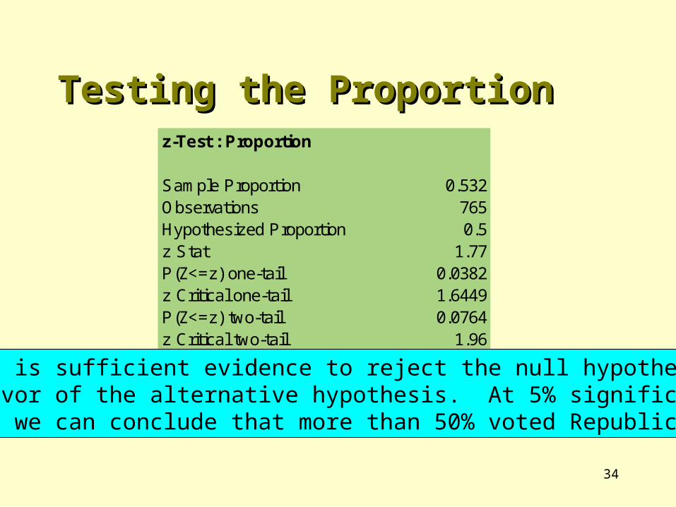
z-Test : Proportion

Sample Proportion 0.532Observations 765Hypothesized Proportion 0.5z Stat 1.77P(Z<=z) one-tail 0.0382z Critical one-tail 1.6449P(Z<=z) two-tail 0.0764z Critical two-tail 1.96

There is sufficient evidence to reject the null hypothesisin favor of the alternative hypothesis. At 5% significance level we can conclude that more than 50% voted Republican.

Testing the ProportionTesting the Proportion

35

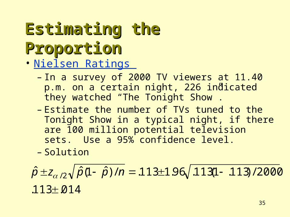
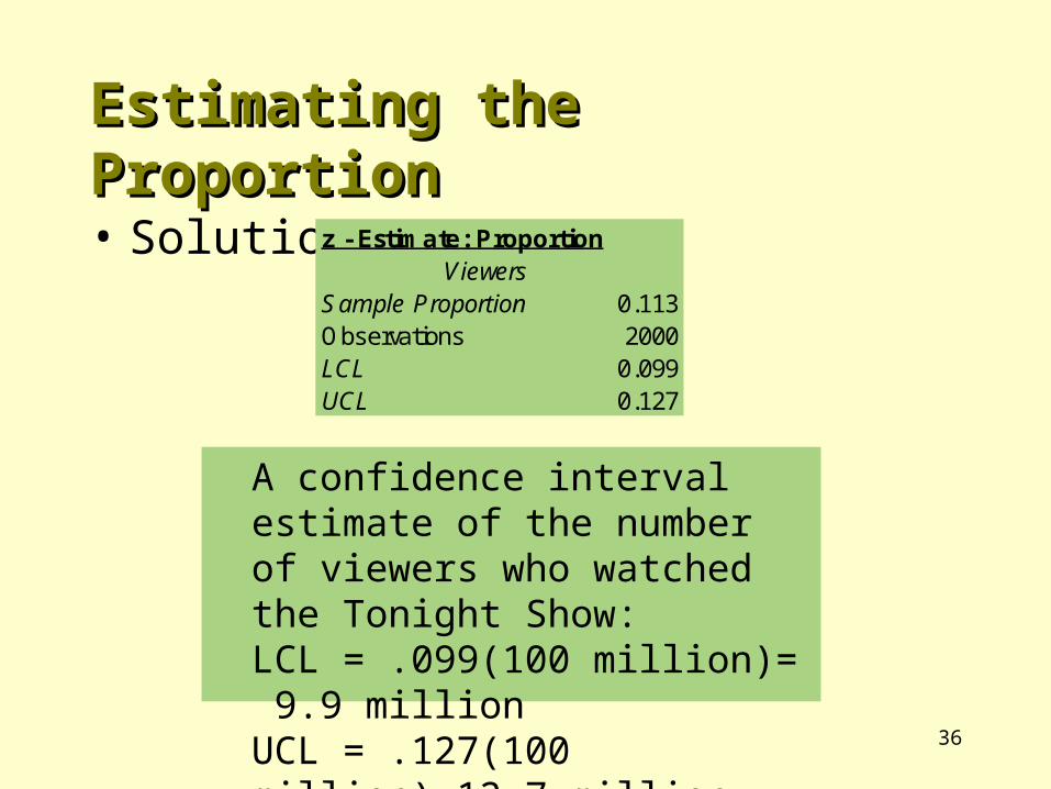
• Nielsen Ratings – In a survey of 2000 TV viewers at 11.40 p.m. on a

certain night, 226 indicated they watched “The Tonight Show”.

– Estimate the number of TVs tuned to the Tonight Show in a typical night, if there are 100 million potential television sets. Use a 95% confidence level.

– Solution

014.113.

2000/)113.1(113.96.1113./)ˆ1(ˆˆ 2/

nppzp

Estimating the ProportionEstimating the Proportion

36

A confidence interval estimate of the number of viewers who watched the Tonight Show:LCL = .099(100 million)= 9.9 millionUCL = .127(100 million)=12.7 million

• Solution

Estimating the ProportionEstimating the Proportion

z - Estimate: ProportionViewers

Sample Proportion 0.113Observations 2000LCL 0.099UCL 0.127

37

Selecting the Sample Size to Estimate Selecting the Sample Size to Estimate the Proportionthe Proportion

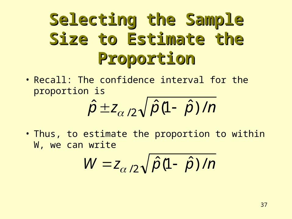
• Recall: The confidence interval for the proportion is

• Thus, to estimate the proportion to within W, we can write

nppzp /)ˆ1(ˆˆ 2/

nppzW /)ˆ1(ˆ2/

38

Selecting the Sample Size to Estimate Selecting the Sample Size to Estimate the Proportionthe Proportion

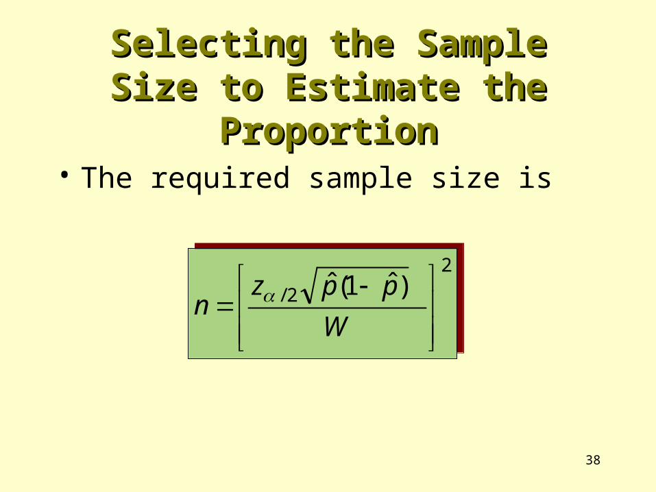
• The required sample size is

2

2/ )ˆ1(ˆ

W

ppzn

2

2/ )ˆ1(ˆ

W

ppzn

39

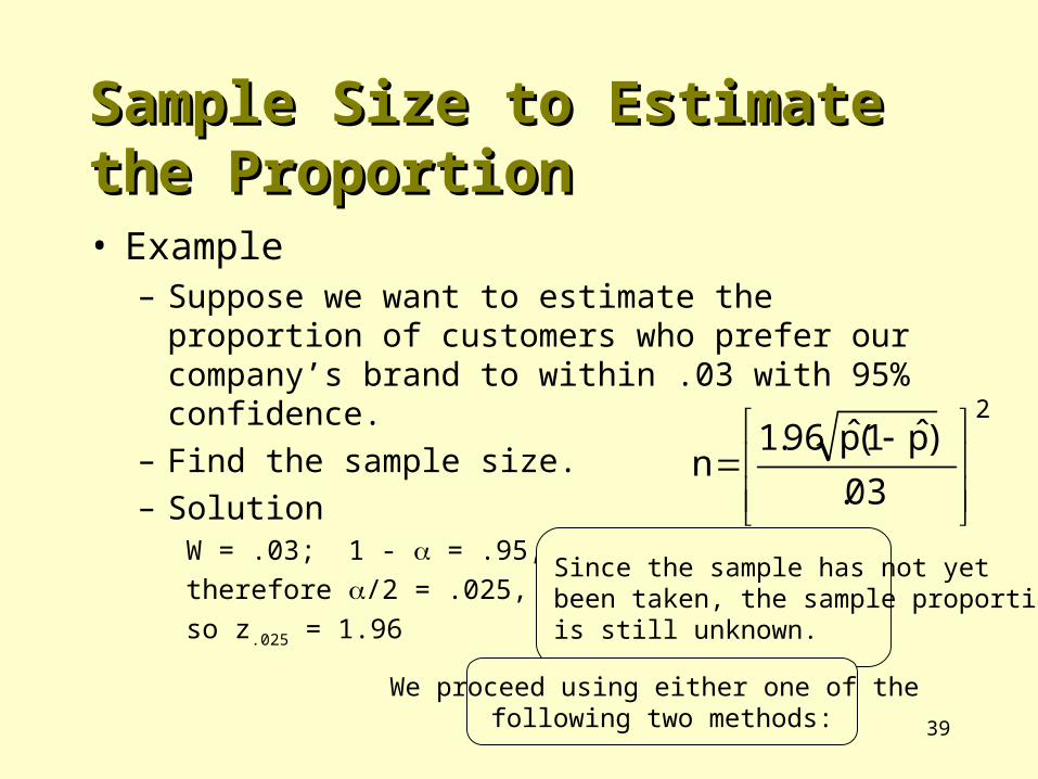
• Example– Suppose we want to estimate the proportion of customers

who prefer our company’s brand to within .03 with 95% confidence.

– Find the sample size.– Solution

W = .03; 1 - = .95, therefore /2 = .025, so z.025 = 1.96

2

03.)p̂1(p̂96.1

n

Since the sample has not yet been taken, the sample proportionis still unknown.

We proceed using either one of the following two methods:

Sample Size to Estimate the ProportionSample Size to Estimate the Proportion

40

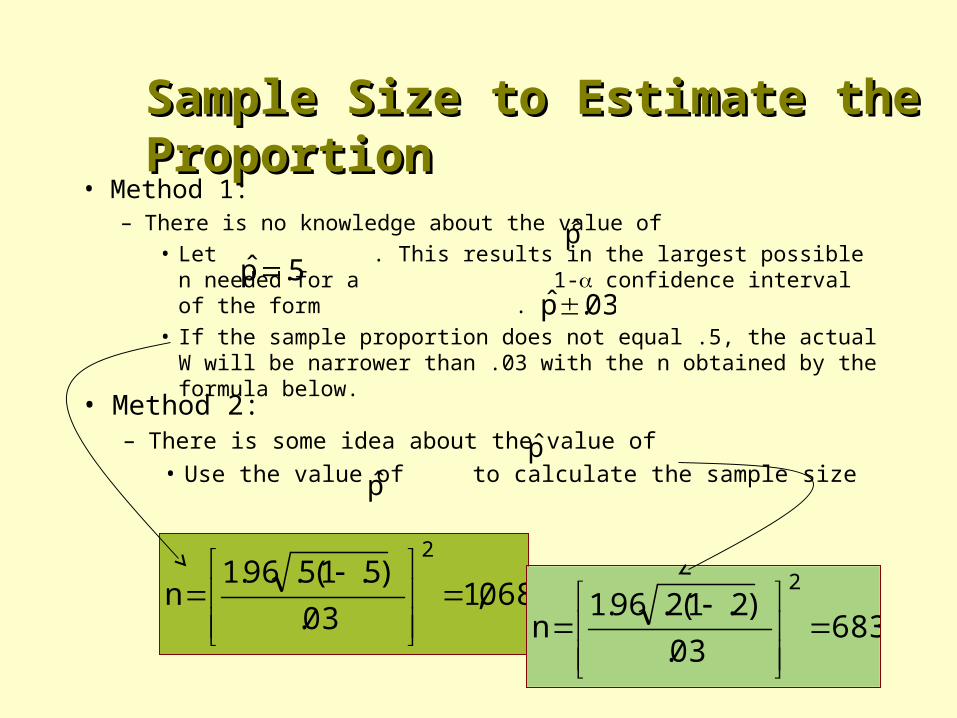
• Method 1:– There is no knowledge about the value of

• Let . This results in the largest possible n needed for a 1- confidence interval of the form .

• If the sample proportion does not equal .5, the actual W will be narrower than .03 with the n obtained by the formula below.

5.p̂ 03.p̂

p̂

068,103.

)5.1(5.96.1n

2

68303.

)2.1(2.96.1n

2

Sample Size to Estimate the ProportionSample Size to Estimate the Proportion

• Method 2:– There is some idea about the value of

• Use the value of to calculate the sample sizep̂p̂