Estimation IIIan Reid

Hilary Term, 2001

1 Discrete-time Kalman filter

We ended the first part of this course deriving the Discrete-Time Kalman Filter as a recursive Bayes’estimator. In this lecture we will go into the filter in more detail, and provide a new derivation forthe Kalman filter, this time based on the idea ofLinear Minimum Variance (LMV) estimation ofdiscrete-time systems.

1.1 Background

The problem we are seeking to solve is the continual estimation of a set of parameters whose valueschange over time. Updating is achieved by combining a set of observations or measurementsz(t)which contain information about the signal of interestx(t). The role of the estimator is to providean estimatex(t+ �) at some timet+ � . If � > 0 we have aprediction filter, if � < 0 asmoothingfilter and if � = 0 the operation is simply calledfiltering .

Recall that an estimator is said to beunbiased if the expectation of its output is the expectation ofthe quantity being estimated,E[x℄ = E[x℄.Also recall that aminimum variance unbiased estimator (MVUE) is an estimator which is unbi-ased and minimises the mean square error:x = argminx E[jjx� xjj2jz℄ = E[xjz℄The termE[jjx � xjj2℄, the so-calledvariance of error, is closely related to theerror covariancematrix ,E[(x� x)(x� x)T ℄. Specifically, the variance of error of an estimator is equalto the traceof the error covariance matrix,E[jjx� xjj2℄ = traceE[(x� x)(x� x)T ℄:The Kalman filter is alinear minimum variance of error filter (i.e. it is the best linear filter over theclass of all linear filters) over time-varying and time-invariant filters. In the case of the state vectorxand the observationsz being jointly Gaussian distributed, the MVUE estimator is alinear functionof the measurement setz and thus the MVUE (sometimes written MVE for Minimum Variance ofError estimator) is also a LMV estimator, as we saw in the firstpart of the course.

1

Notation

The following notation will be used.zk observation vector at timek.Zk the set of all observations up to (and including) timek.xk system state vector at timek.xkji estimation ofx at timek based on timei, k � i.~xkjk estimation error,xkjk � xk; (tilde notation)Pk Covariance matrix.Fk State transition matrix.Gk Input (control) transition matrix.Hk Output transition matrix.wk process (or system, or plant) noise vector.vk measurement noise vector.Qk process (or system, or plant) noise covariance matrix.Rk measurement noise covariance matrix.Kk Kalman gain matrix.�k innovation at timek.Sk innovation covariance matrix at timek.

1.2 System and observation model

We now begin the analysis of the Kalman filter. Refer to figure 1. We assume that the system can bemodelled by the state transition equation,xk+1 = Fkxk +Gkuk +wk (1)

wherexk is the state at timek, uk is an input control vector,wk is additive system or process noise,Gk is the input transition matrix andFk is the state transition matrix.

We further assume that the observations of the state are madethrough a measurement system whichcan be represented by a linear equation of the form,zk = Hkxk + vk; (2)

wherezk is the observation or measurement made at timek, xk is the state at timek, Hk is theobservation matrix andvk is additive measurement noise.

2

++

+

+ +Hunit

delay

F

Gu

w

x z

v

Figure 1:State-space model.

1.3 Assumptions

We make the following assumptions;� The process and measurement noise random processeswk andvk are uncorrelated, zero-meanwhite-noise processes with known covariance matrices. Then,E[wkwTl ℄ = � Qk k = l;0 otherwise; (3)E[vkvTl ℄ = � Rk k = l;0 otherwise; (4)E[wkvTl ℄ = 0 for all k; l (5)

whereQk andRk are symmetric positive semi-definite matrices.� The initial system state,x0 is a random vector that is uncorrelated to both the system andmeasurement noise processes.� The initial system state has a known mean and covariance matrixx0j0 = E[x0℄ and P0j0 = E[(x0j0 � x0)(x0j0 � x0)T ℄ (6)

Given the above assumptions the task is to determine, given aset of observationsz1; : : : ; zk+1, theestimation filter that at thek + 1th instance in time generates an optimal estimate of the statexk+1,which we denote byxk+1, that minimises the expectation of the squared-error loss function,E[jjxk+1 � xk+1jj2℄ = E[(xk+1 � xk+1)T (xk+1 � xk+1)℄ (7)

1.4 Derivation

Consider the estimation of statexk+1 based on the observations up to timek, z1 : : : ; zk , namelyxk+1jZk . This is called a one-step-ahead prediction or simply aprediction. Now, the solution tothe minimisation of Equation 7 is the expectation of the state at timek + 1 conditioned on theobservations up to timek. Thus,

3

xk+1jk = E[xk+1jz1; : : : ; zk ℄ = E[xk+1jZk℄ (8)

Then the predicted state is given byxk+1jk = E[xk+1jZk℄= E[Fkxk +Gkuk +wkjZk℄= FkE[xkjZk ℄ +Gkuk +E[wkjZk ℄= Fkxkjk +Gkuk (9)

where we have used the fact that the process noise has zero mean value anduk is known precisely.

The estimate variancePk+1jk is the mean squared error in the estimatexk+1jk.

Thus, using the facts thatwk andxkjk are uncorrelated:Pk+1jk = E[(xk+1 � xk+1jk)(xk+1 � xk+1jk)T jZk℄= FkE[(xk � xkjk)(xk � xkjk)T jZk℄FTk +E[wkwTk ℄= FkPkjkFTk +Qk (10)

Having obtained a predictive estimatexk+1jk suppose that we now take another observationzk+1.How can we use this information to update the prediction, ie.find xk+1jk+1? We assume that theestimate is a linear weighted sum of the prediction and the new observation and can be described bythe equation, xk+1jk+1 = K0k+1xk+1jk +Kk+1zk+1 (11)

whereK0k+1 andKk+1 are weighting orgain matrices (of different sizes). Our problem now is toreduced to finding theKk+1 andK0k+1 that minimise the conditional mean squared estimation errorwhere of course the estimation error is given by:~xk+1jk+1 = xk+1jk+1 � xk+1 (12)

1.5 The Unbiased Condition

For our filter to be unbiased, we require thatE[xk+1jk+1℄ = E[xk+1℄. Let’s assume (and argueby induction) thatxkjk is an unbiased estimate. Then combining equations (11) and (2) and takingexpectations yieldsE[xk+1jk+1℄ = E[K0k+1xk+1jk +Kk+1Hk+1xk+1 +Kk+1vk+1℄= K0k+1E[xk+1jk ℄ +Kk+1Hk+1E[xk+1℄ +Kk+1E[vk+1℄ (13)

Note that the last term on the right hand side of the equation is zero, and further note that theprediction is unbiased: E[xk+1jk ℄ = E[Fkxkjk +Gkuk℄= FkE[xkjk ℄ +Gkuk= E[xk+1℄ (14)

4

Hence by combining equations (13) and (14))E[xk+1jk+1℄ = (K0k+1 +Kk+1Hk+1)E[xk+1℄and the condition thatxk+1jk+1 be unbiased reduces the requirement toK0k+1 +Kk+1Hk+1 = I

or K0k+1 = I�Kk+1Hk+1 (15)

We now have that for our estimator to be unbiased is must satisfyxk+1jk+1 = (I�Kk+1Hk+1)xk+1jk +Kk+1zk+1= xk+1jk +Kk+1[zk+1 �Hk+1xk+1jk ℄ (16)

whereK is known as theKalman gain.

Note that sinceHk+1xk+1jk can be interpreted as a predicted observationzk+1jk , equation 16 canbe interpreted as the sum of a prediction and a fraction of thedifference between the predicted andactual observation.

1.6 Finding the Error Covariance

We determined the prediction error covariance in equation (10). We now turn to the updated errorcovariancePk+1jk+1 = E[~xk+1jk+1~xk+1jk+1)T jZk ℄= E[(xk+1 � xk+1jk+1)(xk+1 � xk+1jk+1)T ℄= (I�Kk+1Hk+1)E[~xk+1jk~xTk+1jk℄(I�Kk+1Hk+1)T+Kk+1E[vk+1vTk+1℄KTk+1 + 2(I�Kk+1Hk+1)E[~xk+1jkvTk+1℄KTk+1and with E[vk+1vTk+1℄ = Rk+1E[~xk+1jk~xTk+1jk ℄ = Pk+1jkE[~xk+1jkvTk+1℄ = 0we obtainPk+1jk+1 = (I�Kk+1Hk+1)Pk+1jk(I�Kk+1Hk+1)T +Kk+1Rk+1KTk+1 (17)

Thus the covariance of the updated estimate is expressed in terms of the prediction covariancePk+1jk , the observation noiseRk+1 and the Kalman gain matrixKk+1.

1.7 Choosing the Kalman Gain

Our goal is now to minimise the conditional mean-squared estimation error with respect to theKalman gain,K.

5

L = minKk+1E[~xTk+1jk+1~xk+1jk+1jZk+1℄= minKk+1 trace�E[~xk+1jk+1~xTk+1jk+1jZk+1℄�= minKk+1 trace�Pk+1jk+1� (18)

For any matrixA and a symmetric matrixB��A �trace(ABAT )� = 2AB(to see this, consider writing the trace as

Pi aTi Bai whereai are the columns ofAT , and thendifferentiating w.r.t. theai).Combining equations (17) and (18) and differentiating withrespect to the gain matrix (using therelation above) and setting equal to zero yields�L�Kk+1 = �2(I�Kk+1Hk+1)Pk+1jkHTk+1 + 2Kk+1Rk+1 = 0Re-arranging gives an equation for the gain matrixKk+1 = Pk+1jkHTk+1[Hk+1Pk+1jkHTk+1 +Rk+1℄�1 (19)

Together with Equation 16 this defines the optimal linear mean-squared error estimator.

1.8 Summary of key equations

At this point it is worth summarising the key equations whichunderly the Kalman filter algorithm.The algorithm consists of two steps; a prediction step and anupdate step.

Prediction: also known as the time-update. This predicts the state and variance at timek + 1dependent on information at timek.xk+1jk = Fkxkjk +Gkuk (20)Pk+1jk = FkPkjkFTk +Qk (21)

Update: also known as the measurement update. This updates the stateand variance using acombination of the predicted state and the observationzk+1.xk+1jk+1 = xk+1jk +Kk+1 �zk+1 �Hk+1xk+1jk� (22)Pk+1jk+1 = (I�Kk+1Hk+1)Pk+1jk(I�Kk+1Hk+1)T +Kk+1Rk+1KTk+1 (23)

6

++

+Hunit

delay FGu

Blending

stateestimate

x

K

z

measurement

z

measurementprediction

state predictioncorrection

innovation(whitening)

+−

Figure 2:Discrete-time Kalman filter block diagram.

where the gain matrix is given byKk+1 = Pk+1jkHTk+1[HkPk+1jkHTk+1 +Rk+1℄�1 (24)

Together with the initial conditions on the estimate and itserror covariance matrix (equation 6)this defines the discrete-time sequential, recursive algorithm for determining the linear minimumvariance estimate known as the Kalman filter.

1.9 Interpreting the Kalman Filter

We now take a look at the overall Kalman filter algorithm in more detail. Figure 2 summarises thestages in the algorithm in block diagram form.

The innovation, �k+1, is defined as the difference between the observation (measurement)zk+1and its predictionzk+1jk made using the information available at timek. It is a measure of the newinformation provided by adding another measurement in the estimation process.

Given that zk+1jk = E[zk+1jZk ℄= E[Hk+1xk+1 + vk+1jZk℄= Hk+1xk+1jk (25)

the innovation�k+1 can be expressed by�k+1 = zk+1 �Hk+1xk+1jk (26)

The innovation or residual is an important measure of how well an estimator is performing. Forexample it can be used to validate a measurement prior to it being included as a member of theobservation sequence (more on this later).

7

The process of transformingzk+1 into �k+1 is sometimes said to be achieved through theKalmanwhitening filter . This is because the innovations form an uncorrelated orthogonal white-noise pro-cess sequenceVk+1 which is statistically equivalent to the observationsZk+1. This is importantbecause where aszk+1 is in generally statistically correlated, the innovation�k+1 is uncorrelated soeffectively provides new information or “innovation”.

The innovation has zero mean, since,E[�k+1jZk℄ = E[zk+1 � zk+1jkjZk ℄= E[zk+1jZk℄� zk+1jk ;= 0 (27)

and the innovation varianceSk+1 is given bySk+1 = E[�k+1�Tk+1℄;= E[(zk+1 �Hk+1xk+1jk)(zk+1 �Hk+1xk+1jk)T ℄Sk+1 = Rk+1 +Hk+1Pk+1jkHTk+1 (28)

Using Equation 26 and 28 we can re-write the Kalman updates interms of the innovation and itsvariance as follows.xk+1jk+1 = xk+1jk +Kk+1�k+1 (29)Pk+1jk+1 = E[(xk+1 � xk+1jk �Kk+1�k+1)(xk+1 � xk+1jk �Kk+1�k+1)T ℄= E[(xk+1 � xk+1jk)(xk+1 � xk+1jk)T ℄�Kk+1E[�k+1�Tk+1℄Pk+1jk+1 = Pk+1jk �Kk+1Sk+1KTk+1 (30)

where, from Equation 19 Kk+1 = Pk+1jkHTk+1S�1k+1 (31)

and Sk+1 = Hk+1Pk+1jkHTk+1 +Rk+1: (32)

This is a convenient form of the Kalman filter often used in analysis.

Although primarily used as a state estimator the Kalman filter algorithm can be used to estimateparameters other than the state vector. These are illustrated in Figure 2.

1. If applied to estimatezk+1jk it is called ameasurementfilter.

2. If applied to estimatexk+1jk it is called aprediction filter.

3. If applied to estimate�k+1 it is called awhitening filter.

4. If applied to estimatexk+1jk+1 it is called aKalman filter.

1.10 Example

Consider a vehicle tracking problem where a vehicle is constrained to move in a straight line witha constant velocity. Letp(t) and _p(t) represent the vehicle position and velocity. We assume thatobservations of position can be made where the measurement noise isv(t). Since the vehicle ismoving at constant speed,�p(t) = 0.

8

System model: The system state can be described byx(t) = [p(t); _p(t)℄T . The system state andoutput equations can be expressed by_x(t) = Ax(t) +w(t);z(t) = Hx(t) + v(t); (33)

where A = � 0 10 0 � ; H = � 1 0 � :Suppose we have sampled observations of the system at discrete time intervals4T , then the discreteequivalent is given by (see later this lecture for a derivation)xk+1 = Fkxk +wk (34)

where Fk = eA4T = �1 4T0 1 � (35)zk = Hxk + vk (36)

Kalman filter: Suppose that the known mean and covariance ofx0 = x(0) are,x0j0 = E(x0) = � 010� P0j0 = �10 00 10� (37)

Assume also that Qk = E(wkwTk ) = �1 00 1� Rk = E(v2k) = 1 (38)

The Kalman filter involves sequential application of the recursive equations as given above fork =0; 1; : : : . Here is some Matlab code to implement them, and an example program

function [xpred, Ppred] = predict(x, P, F, Q)

xpred = F*x;Ppred = F*P*F’ + Q;

function [nu, S] = innovation(xpred, Ppred, z, H, R)

nu = z - H*xpred; %% innovationS = R + H*Ppred*H’; %% innovation covariance

function [xnew, Pnew] = innovation_update(xpred, Ppred, n u, S, H)

K = Ppred*H’*inv(S); %% Kalman gainxnew = xpred + K*nu; %% new statePnew = Ppred - K*S*K’; %% new covariance

9

%%% Matlab script to simulate data and process usiung Kalman filter

delT = 1;F = [ 1 delT

0 1 ];H = [ 1 0 ];x = [ 0

10];P = [ 10 0

0 10 ];Q = [ 1 1

1 1 ];R = [ 1 ];z = [2.5 1 4 2.5 5.5 ];

for i=1:5[xpred, Ppred] = predict(x, P, F, Q);[nu, S] = innovation(xpred, Ppred, z(i), H, R);[x, P] = innovation_update(xpred, Ppred, nu, S, H);

end

Results: The plots in Figure 3a-c illustrate the result of running theKalman filter using�t = 1.Some interesting observations can be made as follows.

1. BothKk+1 andPk+1jk+1 tend to constant (steady-state) values ask !1.

2. The estimatesxk+1jk+1 tend to follow the measurement values quite closely. IndeedsinceKk+1 is a weighting function acting on the measurement it is clearthat this effect is moreprominent whenKk+1 is high.

3. From Equation 19Kk+1 is decreases withRk+1 and increases withQk+1. Thus the conver-gence properties are dependent on the relative magnitudes of the process and measurementnoise. Figure 4a illustrates this effect clearly. Here we have re-run the Kalman filter but de-creased the elements ofQk+1 by a factor of 10 and 100 (Rk+1 was kept at the original value).It is clear from the figure that the net effect is that the estimates follow the measurements lessclosely. Similar effects can be observed if the relative magnitude ofRk+1 is increased (Figure4b). How do you explain what is observed in the latter case?

This example illustrates the fact that the performance of a Kalman filter is dependent on initialisationconditions. In the next lecture we examine this observationin more detail when we consider theperformance of the discrete-time Kalman filter.

1.11 Deriving the System Model

Up to this point we have somewhat glossed over the derivationof the discrete system evolutionmodel, but since there are one or two points which are not entirely obvious, we illustrate it here withsome examples.

10

(a)

0

1

2

3

4

5

6

0 1 2 3 4 5

x(k)^

k

z(k)

(b)

0.4

0.5

0.6

0.7

0.8

0.9

1.0

0 1 2 3 4 5

k

K0

K1

(c)

0

1

2

3

4

5

6

7

0 1 2 3 4 5

k

P(k|k)11

P(k|k)00

Figure 3:Example 1: (a) measurement and estimated state trajectories; (b) Kalman gain; (c) diago-nal elements of error covariance matrix. Note how in the latter diagrams the curves tend to constantvalues ask gets large.

0

1

2

3

4

5

6

0 1 2 3 4 5

k

alpha=1

alpha=0.1

alpha=0.01

z(k)

0

1

2

3

4

5

6

7

8

9

10

11

12

0 1 2 3 4 5

k

beta=1

beta=100

z(k)

Figure 4: Example 1: Effect of changing the process and measurement noise covariance matriceson the estimated position trajectory. (a) decreasingQk+1 by a factor of 10 and 100; (b) increasingRk+1 by a factor of 100.

11

1.11.1 Constant-velocity particle

Consider a particle moving at constant velocity. It’s idealmotion is described by�x(t) = 0. In thereal world, the velocity will undergo some perturbationw(t) which we will assume to be randomlydistributed. Therefore the real motion equation is given by,�x(t) = w(t)where E[w(t)℄ = 0E[w(t)w(�)℄ = q(t)Æ(t� �)Recall from your 2nd year maths that this latter expectationis theauto-correlation function and thatan autocorrelation of this form corresponds to aconstant power spectral density, more commonlyreferred to aswhite noise.

The state vector is, x = �x_x� (39)

and the continuous state-space system equation is�x�t = Ax(t) +Bw(t) (40)

where A = �0 10 0� and B = �01� (41)

We obtain the discrete time equivalent for equation 40 for a sample interval of�t by integating upover one sampling period. Taking Laplace transforms we obtain:sX(s)� x(0) = AX(s) +BW(s)) (sI�A)X(s) = x(0) +BW(s)) X(s) = (sI�A)�1x(0) + (sI�A)�1BW(s)Now taking inverse Laplace transforms:x(�t) = �1 �t0 1 �x(0) + Z �t0 �1 �t� �0 1 �Bw(�)d�Note that the integration on the right hand side is a consequence of the convolution rule for Laplacetransforms.

Shifting this forward in time to match our initial conditions we havex(tk +�t) = �1 �t0 1 �x(tk) + Z �t0 �1 �t� �0 1 �Bw(tk + �)d�= �1 �t0 1 �x(tk) + Z �t0 ��t� �1 �w(tk + �)d�or xk+1 = Fk xk + wk (42)

12

It remains to determine the process noise covariance,Qk = E[wkwTk ℄:Qk = E[wkwTk ℄= E[(Z �t0 ��t� u1 �w(tk + u)du)(Z �t0 ��t� v1 �w(tk + v)dv)T ℄= Z �t0 Z �t0 ��t� u1 � ��t� v 1�E[w(tk + u)w(tk + v)T ℄dudv= Z �t0 �(�t� u)2 (�t� u)(�t� u) 1 � q(tk + u)du= q � 13�t3 12�t212�t2 �t � (43)

since (by our initial assumptions)q is constant.

In summary: Fk = �1 �t0 1 � and Qk = q � 13�t3 12�t212�t2 �t � (44)

Note that we have derived the process noise covariance usinga continuous-time white noiseas-sumption. If, on the other hand we assume apiece-wise constant white noisemodel, then the targetundergoes a constant accelerationwk, with the accelerations independent from period to period,andthe process noise is slightly different. Bar-Shalom (p86) discusses (and derives the piecewise ver-sion) this and you should familiarise yourselves with both,but always keeeping in mind that bothare approximations.

1.11.2 Constant-acceleration particle

The analysis is similar to the previous case. In this case theparticle moves at constant acceleration.The ideal particle motion is described by��x(t)=�t = 0. In the real world, the acceleration will notbe perfectly constant, thus, ��x(t)�t = w(t);where as before, E[w(t)℄ = 0;E[w(t)w(�)℄ = q(t)Æ(t� �)We can express the state-space model of the system as follows.

The state vector is x = 24 x_x�x 35 (45)

The continuous state-space system equation is,�x�t = Ax(t) +Bw(t); (46)

13

where A = 24 0 1 00 0 10 0 0 35 and B = 2400135 (47)

The discrete-time equivalent to Equation 46 for a sample interval of�t is given by,xk+1 = Fkxk +wk (48)

Once again taking Laplace transforms (etc) and using the assumption thatq is constant, we candetermine the state transition matrixFk and the process noise covariance matrixQk:Fk = eA�t = 241 �t �t20 1 �t0 0 1 35

and Qk = E[wkwTk ℄ = q 24�t5=20 �t4=8 �t3=6�t4=8 �t3=3 �t2=2�t3=6 �t2=2 �t 35 (49)

2 Kalman Filter Performance

In this lecture we consider how to evaluate the performance of a Kalman filter. We will focus onunderstanding the following problems

1. how a Kalman filter of a perfectly modelled system with perfectly estimated noise behaves.

2. the effect that changes in the values of the noise sources have on the overall performance of aKalman filter.

3. how to recognise if the filter assumptions are met in practice. This is particularly importantin practical situations since many real systems are not wellrepresented by a linear model andmeasurement and system noise is non-Gaussian.

In the case of (3), here, we will only consider how to detect a problem with a Kalman filter. We con-sider how to modify the Kalman filter to accommodate nonlinear process and measurement modelsand non-Gaussian noise in the final lecture.

2.1 Example

We will illustrate Kalman filter performance using as an example a variant of the constant velocitymodel we considered in section 1.10, in which we use the Kalman filter to track a vehicle moving ina straight line.

14

(a)

-10

0

10

20

30

40

50

60

70

10 20 30 40 50 60 70 80 90 100

(b)

-0.2

0.0

0.2

0.4

0.6

0.8

1.0

1.2

1.4

1.6

10 20 30 40 50 60 70 80 90 100

(c)

-10

0

10

20

30

40

50

60

70

10 20 30 40 50 60 70 80 90 100

Figure 5:Input to Example 2: (a) true position; (b) true velocity; (c)observations.

System model

We assume that sampled observations are acquired at discrete time intervals�t and the system stateand output equations are of the formxk+1 = �1 �t0 1 �xk +wk (50)zk = �1 0�xk + vk: (51)

Further, we assume that the process and observation noise are given byQk = ��T 3=3 �T 2=2�T 2=2 �T ��2q Rk = �2r : (52)

We will take�2q = 0:01, �2r = 0:1 and assume that the vehicle starts from rest so thatx0j0 = [0; 0℄T .Figure 5 shows the true position and velocity and observations for a run of 100 samples computedfrom the system equations using a pseudo-randomnumber generator to generate normally distributedrandom numbers for the variances�2r and�2q .

15

2.2 Performance under ideal modelling conditions

We first consider the performance of the Kalman filter under ideal modelling conditions meaningthat the system model is known precisely as are the process and noise models.

Figure 6 shows the position track achieved by applying the Kalman filter. Figure 6a shows thepredicted and estimated positions together with the measurements for the complete track. A close-up of the initial track is shown in Figure 6b. The key thing to note here is that the updated estimatexk+1jk+1 always lies between the predictionxk+1jk and the measurementzk+1. This follows fromthe fact that the update is a weighted sum of the prediction and the measurement (see lecture 1).Figure 6c shows a close-up of the estimator when it is in the steady-state. In this case, the weights(i.e. the Kalman gain) used in the update are approximately constant.

Figure 7 shows the velocity track achieved by applying the Kalman filter. No measurement is madeof the velocity state so estimates are produced via the cross-correlation between the velocity andposition (ie throughP).

2.2.1 Steady-state performance

Figure 8 shows the predicted and estimated error covariances for position and velocity. In particular,note that they tend to constant values ask gets large.

Performance in the steady-state turns out to be dependent onthe values chosen for the process andmeasurement noise covariance matrices,Q andR.

Given that Pk+1jk = FkPkjkFTk +Qkand Pkjk = Pkjk�1 �Pkjk�1HTk [HkPkjk�1HTk +Rk℄�1HkPkjk�1we havePk+1jk = Fk[Pkjk�1 �Pkjk�1HTk [HkPkjk�1HTk +Rk℄�1HkPkjk�1℄FTk +Qk (53)

Equation (53) is known as the discrete-timematrix Ricatti equation . It turns out that if the system istime-invariant (i.e.F;G; andH are constant), and the measurement and process noise are stationary(Q andR are constant) then ask !1 the solution to equation (53) converges to a positive definitematrix �P provided that the system model is completelyobservableand completelycontrollable (forprecise definitions of these see Jacobs). The correspondinggain matrix�K = �PHTS�1 will also beconstant and called thesteady-state gain.

The importance of this result is that in some applications you can assume that the Kalman filterworks under steady-state conditions. In this case you fix thevalue of�P and hence�K from the startand initial conditions do not need to be specified. SinceK is now fixed it means that considerablecomputational saving can be made sinceK does not have to be recomputed at each time step.

2.2.2 Initialisation

Recall that part of the requirements for a Kalman filter is specification of initial conditions. There-fore, when considering implementation of a Kalman filter an important concern is how to set (guess!)

16

(a)

−10

0

10

20

30

40

50

60

70

10 20 30 40 50 60 70 80 90 100

(b)

-0.6

-0.4

-0.2

0.0

0.2

0.4

0.6

0.8

1.0

2 3 4 5 6 7 8 9 10

(c)

39

40

41

42

43

44

45

46

47

48

49

50

74 76 78 80 82 84 86

Figure 6:Position track: (a) predicted, estimated positions and observation ; (b) initial track (zoomof (a)); (c) steady-state track (zoom of (a).

−0.2

0.0

0.2

0.4

0.6

0.8

1.0

1.2

1.4

1.6

10 20 30 40 50 60 70 80 90 100

prediction

estimate

Figure 7:Velocity track.

17

(a)

0.0e+00

5.0e−02

1.0e−01

1.5e−01

2.0e−01

0 10 20 30 40 50 60 70 80 90 100

Prediction

Estimate

(b)

0.0e+00

5.0e−02

1.0e−01

1.5e−01

2.0e−01

0 10 20 30 40 50 60 70 80 90 100

EstimatePredication

Figure 8:(a) Position error covariance; (b) Velocity error covariance.

values forx0j0 andP0j0 as they are not known. The obvious question to ask then, is does it matterhow good (or bad) your guess is?

One possibility is to initialise the state vector from the measurementsx0j0 = � z0z0�z�1�t �and a simple way to initialise the state covariance matrix isto set it to be a multipleR of the processnoise matrix P0j0 = RQk;whereR is a constant (typicallyR = 10).

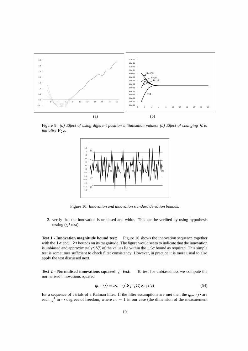
Figure 9 illustrates the effect that changing initialisation parameters has on long term Kalman filterperformance. Note that regardless of the initial values both x andP tend to constant values in a fewiterations.

More formally, it can be shown that provided that the system is observable and controllable the errordue to poor initialisation tends to zero ask ! 1. Finally note that although good initialisationis desirable for a linear Kalman filter it is not essential (the estimator merely takes longer to settledown). However, good initialisation is critical in the implementation of Kalman filters for nonlinearsystem models (see final lecture).

2.2.3 Checking consistency

Since in practice we can not measure performance with respect to the state error measures (sincewe don’t know the true state values) how do we check that the filter is performing correctly? Theanswer is that we can define filter performance measures in terms of theinnovation

We know that if the filter is working correctly then�k is zero mean and white with a covarianceSk(see previous lecture). So we can verify that the filter is consistent by applying the following twoprocedures.

1. check that the innovation is consistent with its covariance by verifying that the magnitude ofthe innovation is bounded by�2pSk.

18

-0.5

0.0

0.5

1.0

1.5

2.0

2.5

3.0

3.5

2 4 6 8 10 12 14 16 18 20

0.0e+00

1.0e−02

2.0e−02

3.0e−02

4.0e−02

5.0e−02

6.0e−02

7.0e−02

8.0e−02

9.0e−02

1.0e−01

1.1e−01

1.2e−01

1.3e−01

0 2 4 6 8 10 12 14 16 18 20

R=100

R=20R=10

R=1

(a) (b)

Figure 9: (a) Effect of using different position initialisation values; (b) Effect of changingR toinitialiseP0j0.

−1.2

−1.0

−0.8

−0.6

−0.4

−0.2

0.0

0.2

0.4

0.6

0.8

1.0

1.2

10 20 30 40 50 60 70 80 90 100

Figure 10:Innovation and innovation standard deviation bounds.

2. verify that the innovation is unbiased and white. This canbe verified by using hypothesistesting (�2 test).

Test 1 - Innovation magnitude bound test: Figure 10 shows the innovation sequence togetherwith the�� and�2� bounds on its magnitude. The figure would seem to indicate that the innovationis unbiased and approximately95% of the values lie within the�2� bound as required. This simpletest is sometimes sufficient to check filter consistency. However, in practice it is more usual to alsoapply the test discussed next.

Test 2 - Normalised innovations squared�2 test: To test for unbiasedness we compute thenormalised innovations squaredqk+1(i) = �k+1(i)S�1k+1(i)�k+1(i) (54)

for a sequence ofi trials of a Kalman filter. If the filter assumptions are met then theqk+1(i) areeach�2 in m degrees of freedom, wherem = 1 in our case (the dimension of the measurement

19

0

1

2

3

4

5

6

7

8

0 10 20 30 40 50 60 70 80 90 100

Figure 11:Normalised innovation and moving average.

vector). Thus E[qk+1℄ = m (55)

This provides the test for unbiasedness. To estimate the mean we need to haveN independentsamples ofqk+1(i); i = 1; : : :N . The mean of this sequence,�qk+1 = 1N NXi=1 qk+1(i)can be used as a test statistic sinceN �qk+1 is �2 onNm degrees of freedom.

In our case, however, we can exploit the fact that the innovations areergodic to estimate the samplemean from the time average for a long sequence (ie. the movingaverage) rather than an ensembleaverage. Thus we can estimate the mean as,�q = 1N NXk=1 qk (56)

from a single run of a Kalman filter. Figure 11 shows the normalised innovation and the movingaverage of the innovation. The latter tends to1:0 ask gets large. To test unbiasedness we need toverify that �q lies in the confidence interval[r1; r2℄ defined by the hypothesisH0 thatN �q is �2Nmdistributed with probability1� �. Thus we need to find[r1; r2℄ such thatP (N �q 2 [r1; r2℄jH0) = 1� �; (57)

For the example we are considering,N = 100, �q = 1:11, and let� = 0:05 (ie. define the two-sided95% confidence region). Using statistical tables we find that,[r1; r2℄ = ��2100(0:025); �2100(0:975)� ;= [74:22; 129:6℄The hypothesis is indeed acceptable for this example.

20

-0.4

-0.2

0.0

0.2

0.4

0.6

0.8

1.0

10 20 30 40 50 60 70 80 90 100

Figure 12:Autocorrelation of the innovation.

Test 3 - Innovation whiteness (autocorrelation) test: To test for whiteness we need to provethat E[�Ti �j ℄ = SiÆij (58)

We can test this by checking that everywhere except wherei = j, the statistic defined by Equation(58) is zero within allowable statistical error. Again, we can exploit ergodicity to redefine the teststatistic as a time-averaged correlationr(�) = 1N N���1Xk=0 �Tk �k+� (59)

The autocorrelation is usually normalised byr(0). Figure 12 shows the normalised auto-correlationof the innovation for the example we are considering. Note that it peaks at� = 0 and everywhereelse is distributed randomly about zero. We can test that theoscillations about zero are random byestimating the variance of the test statistic. For large enoughN we can assume thatr(�) is normallydistributed with mean zero and variance1=N . Then we can compute the2�-gate as�2=pN andcheck that at least95% of the values fall within this confidence region. Again in ourexample theautocorrelation satisfies the hypothesis.

2.3 Model validation

So far we have only considered the performance of a Kalman filter when both the system model andnoise processes are known precisely. A Kalman filter may not perform correctly if there is eithermodelling or noise estimation error or both. Here we discussthe causes and identify most of theimportant techniques used to control a Kalman filter from diverging. We consider two types of errorand their characteristics;

1. Error in the process and observation noise specification.

2. Error in the modelling of system dynamics (process model).

The three tests that we introduced in the last section will beused as a basis for trying to tell whensomething has gone wrong with the filter.

21

2.3.1 Detecting process and observation noise errors

The example used in the previous section will be used to illustrate general characteristics that areobserved when the process and observation noise are under- and over-estimated.

Somematlab code to generate a simulation sequence.

%%% Matlab script to generate some "true" data for later asse ssment%%% Generates:%%% x: the state history which evolves according to%%% x(k+1) = Fx(k) + w(k)%%% w: the process noise history (randomly generated)%%% z: a set of observations on the state corrupted by noise%%% v: the noise on each observation (randomly generated)

N = 100;

delT = 1;F = [ 1 delT

0 1 ];H = [ 1 0 ];sigma2Q = 0.01;sigma2R = 0.1;Q = sigma2Q * [ delTˆ3/3 delTˆ2/2

delTˆ2/2 delT ];P = 10*Q;R = sigma2R * [ 1 ];

x = zeros(2,N);w = zeros(2,N);z = zeros(1,N);v = zeros(1,N);for i=2:N

w(:,i) = gennormal([0;0], Q); % generate process noisex(:,i) = F*x(:,i-1) + w(:,i); % update statev(:,i) = gennormal([0], R); % generate measurement noisez(:,i) = H * x(:,i) + v(:,i); % get "true" measurement

end

plot(x(1,:));

Thematlab code to process the sequence and generate the various graphsis given below.

%%% Matlab script to assess Kalman filter performance%%% The script assumes the existence of a vector z of%%% noise corrupted observations

N = length(z); % number of Klamn filter iterations

Qfactor = 1; % process noise mult factorRfactor = 10; % measurement noise mult factor

delT = 1; % time stepF = [ 1 delT % update matrix

22

0 1 ];H = [ 1 0 ]; % measurement matrix

sigmaQ = Qfactor*sqrt(0.01);sigmaR = Rfactor*sqrt(0.1);Q = sigmaQˆ2 * [ 1/3 1/2 % process noise covariance matrix

1/2 1 ];P = 10*Q;R = sigmaRˆ2 * [ 1 ]; % measurement noise covariance

xhat = zeros(2,N); % state estimatenu = zeros(1,N); % innovationS = zeros(1,N); % innovation (co)varianceq = zeros(1,N); % normalised innovation squared

for i=2:N[xpred, Ppred] = predict(xhat(:,i-1), P, F, Q);[nu(:,i), S(:,i)] = innovation(xpred, Ppred, z(i), H, R);[xhat(:,i), P] = innovation_update(xpred, Ppred, nu, S, R) ;q(:,i) = nu(:,i)’*inv(S(:,i))*nu(:,i);

end

sumQ = sum(q) % determine Sum q which is Chiˆ2 on N d.o.f.r = xcorr(nu); % get autocorrealtion of innovation

plot(xhat(1,:)); % plot state estimatepause;

plot(nu) % plot innovation and 2sigma confidence intervalhold on;plot(2*sqrt(S),’r’);plot(-2*sqrt(S),’r’);hold off;pause;

plot(q); % plot normalised innovation squaredpause;

plot(r(N:2*N-1)/r(N)); % plot autocorr of innovation (nor malised)

Under-estimating�q : Refer to Figure 13. This illustrates the performance tests for the case whenthe process noise is under-estimated by a factor of10.

A greater quantity of innovations than expected (i.e.> 5%) fall outside the2� gate (obvious evenfrom visual inspection).

The normalised innovations squared are larger than expected and the sample mean falls outsidethe confidence bound defined by the�2 test (for my trial the value came to 492.34/100 which isclearly above the 95% confidence region [74.22/100,129.6/100] computed above). This tells us thatthe combined process and measurement noise levels are too low, i.e. too little weight is placed oncurrent measurements in the update process.

The autocorrelation sequence shows time correlations.

23

0 10 20 30 40 50 60 70 80 90 100−10

0

10

20

30

40

50

60

70

0 10 20 30 40 50 60 70 80 90 100−2

−1.5

−1

−0.5

0

0.5

1

1.5

2

(a) (b)

0 10 20 30 40 50 60 70 80 90 1000

5

10

15

20

25

0 10 20 30 40 50 60 70 80 90 100−0.4

−0.2

0

0.2

0.4

0.6

0.8

1

(c) (d)

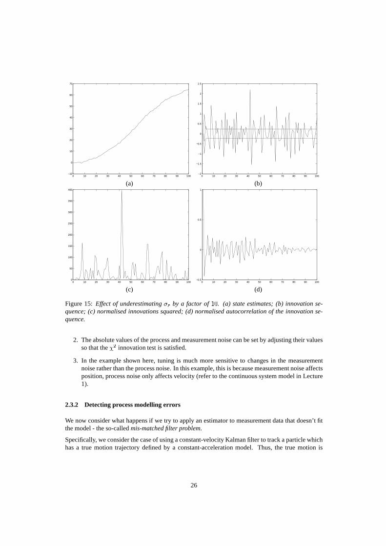
Figure 13:Effect of underestimating�q by a factor of10. (a) state estimates; (b) innovation se-quence; (c) normalised innovations squared; (d) normalised autocorrelation of the innovation se-quence.

Over-estimating�q : Refer to Figure 14. This illustrates the performance tests for the case whenthe process noise is over-estimated by a factor of10. The innovations are well within the requiredbounds.

The normalised innovations squared are smaller than expected and the sum (32.81, or eqivalentlythe average) falls below the confidence bound defined by the�2 test. This tells us that the combinedprocess and measurement noise levels is too high.

The autocorrelation sequence shows no obvious time correlations.

Under-estimating�r: Refer to Figure 15. This illustrates the performance tests for the case whenthe measurement noise is under-estimated by a factor of10.

The innovations exceed the2� bounds more often than allowable.

The normalised innovations squared are larger than expected and the sample mean (3280/100) fallsoutside the confidence bound [0.74,1.3] defined by the�2 test. This tells us that the combinedprocess and measurement noise levels is too low.

24

0 10 20 30 40 50 60 70 80 90 100−10

0

10

20

30

40

50

60

70

0 10 20 30 40 50 60 70 80 90 100−10

−8

−6

−4

−2

0

2

4

6

8

10

(a) (b)

0 10 20 30 40 50 60 70 80 90 1000

0.5

1

1.5

2

2.5

3

3.5

4

0 10 20 30 40 50 60 70 80 90 100−0.5

0

0.5

1

(c) (d)

Figure 14:Effect of overestimating�q by a factor of10. (a) state estimates; (b) innovation sequence;(c) normalised innovations squared; (d) normalised autocorrelation of the innovation sequence.

The autocorrelation sequence shows no obvious time correlations.

Over-estimating�r: Refer to Figure 16. This illustrates the performance tests for the case whenthe measurement noise is over-estimated by a factor of10.

The innovations are below the2� bounds.

The normalised innovations squared are smaller than expected and the sample mean (4.95/100) fallsoutside the confidence bound defined by the�2 test. This tells us that the combined process andmeasurement noise levels is too high.

The autocorrelation sequence shows time correlations.

General observations:

1. If the ratio of process to measurement noise is too low the innovation sequence becomescorrelated.

25

0 10 20 30 40 50 60 70 80 90 100−10

0

10

20

30

40

50

60

70

0 10 20 30 40 50 60 70 80 90 100−2

−1.5

−1

−0.5

0

0.5

1

1.5

2

2.5

(a) (b)

0 10 20 30 40 50 60 70 80 90 1000

50

100

150

200

250

300

350

400

0 10 20 30 40 50 60 70 80 90 100−0.5

0

0.5

1

(c) (d)

Figure 15:Effect of underestimating�r by a factor of10. (a) state estimates; (b) innovation se-quence; (c) normalised innovations squared; (d) normalised autocorrelation of the innovation se-quence.

2. The absolute values of the process and measurement noise can be set by adjusting their valuesso that the�2 innovation test is satisfied.

3. In the example shown here, tuning is much more sensitive tochanges in the measurementnoise rather than the process noise. In this example, this isbecause measurement noise affectsposition, process noise only affects velocity (refer to thecontinuous system model in Lecture1).

2.3.2 Detecting process modelling errors

We now consider what happens if we try to apply an estimator tomeasurement data that doesn’t fitthe model - the so-calledmis-matched filter problem.

Specifically, we consider the case of using a constant-velocity Kalman filter to track a particle whichhas a true motion trajectory defined by a constant-acceleration model. Thus, the true motion is

26

0 10 20 30 40 50 60 70 80 90 100−10

0

10

20

30

40

50

60

70

0 10 20 30 40 50 60 70 80 90 100−8

−6

−4

−2

0

2

4

6

8

(a) (b)

0 10 20 30 40 50 60 70 80 90 1000

0.05

0.1

0.15

0.2

0.25

0 10 20 30 40 50 60 70 80 90 100−0.4

−0.2

0

0.2

0.4

0.6

0.8

1

(c) (d)

Figure 16:Effect of overestimating�r by a factor of10. (a) state estimates; (b) innovation sequence;(c) normalised innovations squared; (d) normalised autocorrelation of the innovation sequence.

described by the transition equation xk+1 = Fxk +wk (60)

where the state transition matrix isF = 241 �T �T 2=20 1 �T0 0 1 35 (61)

with Q = E[wkwTk ℄ = 24�T 5=20 �T 4=8 �T 3=6�T 4=8 �T 3=3 �T 2=2�T 3=6 �T 2=2 �T 35�2q (62)

Figure 17 shows the result of applying the constant-velocity filter to the constant-acceleration modelwhere the filter noise parameters were�q = 0:01 and�r = 0:1.

Observe that the innovation behaves like a first order Gauss-Markov process (recall this implies thatin continuous-timedx=dt + A(t)x = w, wherew is white noise). The normalised squared values

27

0 10 20 30 40 50 60 70 80 90 100−500

0

500

1000

1500

2000

2500

3000

3500

4000

4500

0 10 20 30 40 50 60 70 80 90 100−2

0

2

4

6

8

10

12

(a) (b)

0 10 20 30 40 50 60 70 80 90 1000

50

100

150

200

250

300

350

400

450

500

0 10 20 30 40 50 60 70 80 90 100−0.2

0

0.2

0.4

0.6

0.8

1

1.2

(c) (d)

Figure 17:Performance tests for an unmatched filter. (a) state estimates; (b) innovation sequence;(c) normalised innovations squared; (d) normalised autocorrelation of the innovation sequence.

show a substantial drift in the mean and is not stationary. The autocorrelation reduces exponentiallyin time - again typical of a first-order Gauss-Markov process.

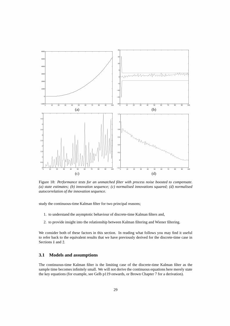
Boosting Q to reduce effects of modelling errors: one obvious thing to try in order to reduce theeffects of modelling errors is to boost the magnitude of the process noiseQ artificially to take intoaccount unmodelled errors. Recall that this should boost the value of the Kalman gain and hence letthe estimate follow the measurements more closely. The result of doing this where the process noisewas increased by a factor of 10 is shown in Figure 18. Some improvement is seen but this has nottotally compensated for the process model error.

3 The Continuous-Time Kalman Filter

So far we have considered the discrete-time formulation of the Kalman filter. This is the versionwhich finds the most wide-spread application in practice. The Kalman filter estimation approachcan also be derived for continuous-time. This is what we lookat in this section. It is interesting to

28

0 10 20 30 40 50 60 70 80 90 100−1000

0

1000

2000

3000

4000

5000

6000

0 10 20 30 40 50 60 70 80 90 100−20

−15

−10

−5

0

5

10

15

20

(a) (b)

0 10 20 30 40 50 60 70 80 90 1000

0.5

1

1.5

2

2.5

3

3.5

4

4.5

5

0 10 20 30 40 50 60 70 80 90 100−0.2

0

0.2

0.4

0.6

0.8

1

1.2

(c) (d)

Figure 18: Performance tests for an unmatched filter with process noiseboosted to compensate.(a) state estimates; (b) innovation sequence; (c) normalised innovations squared; (d) normalisedautocorrelation of the innovation sequence.

study the continuous-time Kalman filter for two principal reasons;

1. to understand the asymptotic behaviour of discrete-timeKalman filters and,

2. to provide insight into the relationship between Kalman filtering and Wiener filtering.

We consider both of these factors in this section. In readingwhat follows you may find it usefulto refer back to the equivalent results that we have previously derived for the discrete-time case inSections1 and2.

3.1 Models and assumptions

The continuous-time Kalman filter is the limiting case of thediscrete-time Kalman filter as thesample time becomes infinitely small. We will not derive the continuous equations here merely statethe key equations (for example, see Gelb p119 onwards, or Brown Chapter 7 for a derivation).

29

In the continuous case thesystem modelis given by�x(t)�t = F(t)x(t) +w(t) (63)

where the process noise has covarianceQ(t).Themeasurement modelis given byz(t) = H(t)x(t) + v(t) (64)

where the measurement noise has covarianceR(t). We assume that the inverseR�1(t) exists.

Recall from the derivation of the discrete-time estimator that we also need to specify initial condi-tions for the state and its error covariance. Thus we assume that the initial conditionsE[x(0)℄ = x(0); E[(x(0)� x(0))(x(0)� x(0))T ℄ = P(0) (65)

are given.

3.2 Kalman filter equations

State estimation is governed by the equation_x(t) = F(t)x(t) +K(t)[z(t) �H(t)x(t)℄ (66)

Error covariance propagation is determined by the differential equation_P(t) = F(t)P(t) +P(t)FT (t) +Q(t)�K(t)R(t)KT (t) (67)

which is known as thematrix Riccati equation. This matrix differential equation has been studiedextensively and an analytic solution exists for the constant parameter case.

Here the Kalman gain matrix is defined byK(t) = P(t)HT (t)R�1(t) (68)

In summary Equations 66, 67 and 68 together with the initial conditions specified by Equation 65describe thecontinuous-time Kalman filter algorithm. You should compare these equations withthe equivalent results for the discrete-time case.

3.3 Example

Consider the problem of estimating the value of a constant signalx(t) given measurements corruptedby Gaussian white noise which is zero-mean and has constant spectral density�. Derive (1) thecontinuous-time Kalman filter; and (2) the discrete-time Kalman filter assuming a sampling timeinterval of�T .

Continuous-time solution: The state-space model equations of the problem are_x(t) = 0 (69)z(t) = x(t) + v(t); v � N(0; �) (70)

30

The scalar Riccati equation (Equation 67) governs error covariance propagation and is given by_p = fp+ pf + q � krk (71)

wherek = ph=r. In this problemf = q = 0; h = 1; r = �. Therefore_p = �k2r and k = p=�Substituting fork and integrating Equation 71 we can solve forp as follows_p = �p2�Z pp0 dpp2 = � 1� Z t0 dt;p = p0(1 + (p0=�) t)�1 (72)

Hence the Kalman gain is given byk = p� = (p0=�)[1 + (p0=�)t℄�1and the state estimation by_x(t) = (p0=�)[1 + (p0=�)t℄�1(z(t)� x(t))Finally, note that ast!1, k ! 0 and the estimate reaches a constant value.

Discrete-time solution: Let us consider what the result would have been if rather thananalysethe continuous-time measurements we had sampled the signals at instants in timet = k�T; k =0; 1; 2; : : : (satisfying the Nyquist criterion of course).

In this case, the discrete-time space-model isx(k + 1) = x(k) (73)z(k) = x(k) + v(k); v(k) � N(0; �) (74)

We haveF(k) =H(k) = 1,Q(k) = 0 andR(k) = �.

The predicted state and error covariance are given by (see Section 1)x(k + 1jk) = x(kjk) andP (k + 1jk) = P (kjk)Using this result the update equation for the error covariance isP (k + 1jk + 1) = P (kjk)�K(k + 1)[�+ P (kjk)℄K(k + 1) (75)

whereK(k+1) = P (kjk)[P (kjk) +�℄�1. Making this substitution forK(k+1) into Equation 75gives P (k + 1jk + 1) = P (kjk) � 11 + P (kjk)=�� : (76)

If our initial error covariance wasP0 then it follows from Equation 76 that, at timek + 1P (k + 1jk + 1) = P0 � 11 + kP0=�� (77)

31

+ +

NV

H_2H_1 YX

Hopt

Figure 19:Wiener filter.

Hence the state update equation isx(k + 1jk + 1) = x(kjk) +K(k + 1) [z(k + 1)� x(kjk)℄ (78)

where K(k + 1) = (P0=�)1 + (kP0=�)Compare this with the result for the continuous-time case. Note again that ask !1, x(k+1jk+1)tends to a constant value.

One final point: unfortunately only simple types of continuous-time problems such as the examplegiven above can be solved analytically using the covarianceequations. For more complicated prob-lems, numerical methods are required. This is the main reason why the continuous-time Kalmanfilter has not found wide-spread use as an estimation method.

3.4 Relation to the Wiener Filter

In this section we consider the connection of the Kalman filter to the Wiener filter. We will not derivethe optimal filter from first principles. Here our interest isin the relation to the Kalman filter.

Problem statement: The Wiener filter is the linear minimum variance of error estimation filterfrom among all time-invariant filters. Briefly, in one-dimension, we consider the problem of howto find the optimal impulse functionh(t) which gives the best estimate of a signals(t) where theinformation available is a corrupted version of the original,z(t) = s(t) + n(t): (79)

Heren(t) is additive noise. If (1) we know the power spectral densities of the signal and noise,SX(s)andSN (s) respectively; and (2) the observations have been acquired for sufficient time length so thatthe spectrum ofz(t) reflects boths(t) andn(t) then the goal is to find the optimal filter responseh(t) to recover the underlying signal.

Wiener filter solution: The Wiener filter solution to this problem is to find the transfer functioncorresponding toh(t) using frequency response methods. It can be shown (see for example Brownchapter 4) that if the signal and noise are uncorrelated thenthe Wiener optimal filter takes on the

32

form HWopt(s) = SX(s)SX(s) + SN (s) (80)

whereSX(s) andSN (s) are the power spectral densities of the signal and noise. However, the filterdefined by Equation 80 defines a non-causal filter, meaning that the output depends on future valuesof the inputz(t) as well as the past, orh(�) 6= 0 for some� � 0For “real-time” operation this filter is not physically realisable (however it can be worth studying foroff-line processing applications). To generate acausalfilter we need to define the filter such that itdepends only on past and current values of the inputz(t), thus,h(�) = 0 for all � � 0Thus we want our optimal filterHWopt(s) to satisfy this. The key is that if a transfer functionF (s)has only poles in the left half plane then its inversef(t) is a positive time function (proof omitted).We can makeHWopt(s) have this property by doing the following.

Consider the denominator of Equation 80. It can be separatedinto a part containing poles and zerosin the left hand plane[SX + SN ℄� and a part containing only poles and zeros in the[SX + SN ℄+.This process is calledspectral decomposition.

Let H1(s) = 1[SX + SN ℄� ; H2(s) = SX[SX + SN ℄+ (81)

Then we can considerHopt as being the cascade of two filters,H1(s) (causal) andH2(s) (non-causal) as illustrated in Figure 19. Letv(t) be the intermediate signal as shown. Then the powerspectral density ofv(t), SV (s) is given bySV (s) = jH1j2(SN + SX)= 1 (82)

In other words it is white noise and hence uncorrelated (independent of time). To make the wholefilter causal we can ignore the negative tail of the impulse response corresponding toH2(s). We dothis by taking partial fractions ofH2(s) and discarding the terms with poles in the right hand plane.We denote this byfH2(s)g�. Hence the causal Wiener optimal filter is given byHWopt(s) = 1[SX(s) + SN (s)℄� � SX(s)[SN (s) + SX(s)℄+�� (83)

Example: As an illustration of this approach consider as an exampleSX(s) = 1�s2 + 1 ; SN (s) = 1 (84)

Then, SN (s) + SX(s) = �s2 + 2�s2 + 1= " (s+p2)(s+ 1) #" (�s+p2)(�s+ 1) # (85)

33

It follows that, H1(s) = (s+ 1)(s+p2) (86)H2(s) is given by H2(s) = 1(�s2+1) (�s+ 1)(�s+p2)= 1(s+ 1)(�s+p2) (87)

Re-writing this equation in partial fractions givesH2(s) = p2� 1s+ 1 + p2� 1�s+p2Hence fH2(s)g� = p2� 1(s+ 1) (88)

Combining Equations 86 and 88 gives the optimal Wiener filterasHWopt(s) = H1(s) fH2(s)g� = (p2� 1)(s+p2) (89)

or in the time domain hWopt(t) = (p2� 1)e�p2t; t � 0 (90)

The Kalman filter equivalent: We can solve the same LMV problem by using an alternativeapproach based on state-space techniques that leads to a Kalman filter solution.

Specifically, we can re-write Equation 79 in terms of a state-space equation asz(t) = Hx(t) + v(t)We can findx as the solution to the steady-state continuous-time Kalmanfiltering problem andhence find the (optimal) transfer function between the signal and measurement. More details ofthis approach are given next followed by a re-working of the example described earlier using thisalternative approach.

We have to make some assumptions about the Kalman filtering problem before we start. Let usassume that the system and measurement equations have linear constant coefficients (i.e.F andHare time-invariant). Let us also assume that the noise processes are time-invariant (Q andR areconstant). Further we assume thatF is controllable, andF andH are observable. Under theseconditions the Kalman filter will reach a steady-state condition where the error covariance matrixP! P1. This means that the matrix Riccati equation (Equation 67) now becomes0 = FP1 +P1FT +Q�K1RKT1;= FP1 +P1FT +Q�P1HTR�1HP1; (91)

34

and state estimation is given by_x(t) = Fx(t) +K1[z(t) �Hx(t)℄ (92)

where the steady-state gain isK1 = P1HTR�1. Equations 91 and 92 define thesteady-state(stationary) continuous-time Kalman filter.

Now let us re-arrange Equation 92_x(t)� (F�K1H)x(t) = K1z(t)Taking the Laplace transform and ignoring initial conditions (since we are in the steady state) wehave (sI� F�K1H)X(s) = K1Z(s)or X(s)Z(s) = HKopt(s) = K1 [(sI� F�K1H)℄�1 (93)

This last equation defines a transfer function between the state estimate and the measurement whichwhen multiplied byH gives theWiener optimal filter ,HWopt(s) =HHKopt(s): (94)

Note that thecausalWiener filter and the continuous-time Kalman filter are equivalent under theassumptions of time-invariance and one can be determined from the other. The key difference is thatone approach is based on state-space models and the other on frequency domain concepts (auto andcross correlations).

Example: Let us re-work the example we considered before using the Kalman filter approach.

The power spectral density ofx(t) is decomposed asSX(s) = 1�s2 + 1 = 1s+ 1 1�s+ 1Thus the state-space model is _x(t) = �x(t) + w(t) (95)z(t) = x(t) + v(t) (96)

Then this implies thatF = �1;Q = 1;H = 1;R = 1.

Substituting these values into the steady-state Riccati equation gives�2P1 �P21 + 1 = 0orP1 = p2� 1. HenceK1 = P1HTR�1 = p2� 1.

The optimal transfer function between the state and measurement is thereforeHKopt(s) = K1 [(sI� F�K1H)℄�1 = p2� 1s+p235

giving HWopt(s) = HHKopt(s) = p2� 1s+p2which agrees with Equation 89.

4 Further Topics in Kalman Filtering

This section deals with some variants of the discrete Kalmanfilter which prove useful when some ofthe assumptions of the conventional Kalman filter break down. Recall that three of the key problemareas for a Kalman filter are,

1. Initialisation: we assume that the initial state vector and its error covariance matrix areknown.

2. Modelling: we assume that we have an accurate linear model of the processand measurementsystem.

3. Noise: we assume that the process and sensor noise processes are Gaussian.

In this section we look at how to deal with each of these problems.

We begin by considering theinformation filter which is a variant on the conventional Kalman filterwhich gives more accurate results when there is no information about the initial state.

Next we consider how to cope with modelling error. In most practical cases the linear equationsdescribing the system and observation models of Equations 14 and 15 in Section1 are not a goodapproximation to reality. Although, as we have seen, it is possible to detect that our assumptionsabout modelling and noise are invalid it is clear that what weneed to do is extend the estimationapproach to accommodate nonlinear models. Recall that for the Kalman filter algorithm, the estimateis the conditional mean of the state given all the measurements up to timek + 1. We showed inSection 1 that under the assumption that the process was linear and the noise processes white thisled to linear, recursive solution of the form,xk+1jk+1 = xk+1jk +Kk+1[zk+1 �Hk+1xk+1jk ℄: (97)

We show that there exists an equivalent version of Equation 97 that can be used in the case of anonlinear system model. We do this by linearising the (non-linear) state and observation matricesabout the estimated trajectory. This leads to the so-calledExtended Kalman Filter (EKF) which isthe best linear estimator with respect to the minimum-mean-square error.

Finally we take a brief look at validating measurements where due to non-Gaussian sensor noisesome measurements could be confused with background clutter or outliers.

4.1 The Information Filter

The information filter (or inverse covariance filter) is an alternative form of the Kalman filter algo-rithm which is mathematically equivalent to the conventional Kalman filter but used in preference toit when either,

36

1. the measurement dimension is large compared to that of theprocess noise; or,

2. the initial system state is unknown.

As with the conventional algorithm, the information filter is a recursive linear estimator that repeat-edly estimates the state of a variable called theinformation vector and its error covariance matrixcalled theinformation matrix . This idea should be familiar from the first part of the coursewherewe discussed recursive least squares.

The information vector at timek + 1 given a set of observations up to this time is defined as�k+1jk+1 = P�1k+1jk+1xk+1jk+1 (98)

It is then straightforward to prove that its covariance is the inverse of the error covariance matrix,P�1k+1jk+1, or information matrix .

Update equations: Recall that the conventional Kalman filter update equation for the error covari-ance matrix is given byPk+1jk+1 = Pk+1jk �Kk+1Hk+1Pk+1jk (99)Kk+1 = Pk+1jkHTk+1(Hk+1Pk+1jkHTk+1 +Rk+1)�1 (100)

The inverse of the (posterior) covariance matrix is given byP�1k+1jk+1 = P�1k+1jk +HTk+1R�1k+1Hk+1 (101)

Proof: [P�PHT (HTPHT +R)�1HP℄[P�1 +HTR�1H℄= I+PHTR�1H�PHT (HTPHT +R)�1H�PHT (HTPHT +R)�1HPHTR�1H= I+PHT [R�1 � (HTPHT +R)�1 � (HTPHT +R)�1HPHTR�1℄H= I+PHT [R�1 � (HTPHT +R)�1(I+HTPHTR�1)℄H= I+PHT [R�1 � (HTPHT +R)�1(R+HTPHT )R�1℄H= I+PHT [I� I℄R�1H= IThe gain can be written Kk+1 = Pk+1jk+1HTk+1R�1k+1 (102)

Proof: K = Pk+1jkHT [HPk+1jkHT +R℄�1= Pk+1jk+1P�1k+1jk+1Pk+1jkHTR�1R[HPk+1jkHT +R℄�1= Pk+1jk+1P�1k+1jk+1Pk+1jkHTR�1[HPk+1jkHTR�1 + I℄�1= Pk+1jk+1[P�1k+1jk +HTR�1H℄Pk+1jkHTR�1[HPk+1jkHTR�1 + I℄�1= Pk+1jk+1[I+HTR�1HPk+1jk℄HTR�1[HPk+1jkHTR�1 + I℄�1= Pk+1jk+1HTR�1[I+HPk+1jkHTR�1℄[HPk+1jkHTR�1 + I℄�1= Pk+1jk+1HTR�137

Next consider how to update the information vector:�k+1jk+1 = P�1k+1jk+1xk+1jk+1= P�1k+1jk+1(I�KH)xk+1jk +P�1k+1jk+1Kz= (P�1k+1jk+1 �HTR�1H)xk+1jk +HTR�1z= P�1k+1jkxk+1jk +HTR�1z (103)

Note that this is exactly the form we derived from Bayes’ Rulein the first part of the course: it is aninformation weighted sum of prediction and measurement

The update can be written succinctly as�k+1jk+1 = �k+1jk +HTk+1R�1k+1zk+1Prediction equations: Recall that the state prediction is defined byxk+1jk = Fxkjk +GuPk+1jk = FPkjkFT +QIt follows that the corresponding prediction equations forthe information filter are�k+1jk = P�1k+1jkFPkjk�kjk +P�1k+1jkGu (104)P�1k+1jk = �FPkjkFT +Q��1 (105)

4.1.1 Summary of key equations

Prediction: �k+1jk = P�1k+1jkFPkjk�kjk +P�1k+1jkGuP�1k+1jk = �FPkjkFT +Q��1Update: P�1k+1jk+1 = P�1k+1jk +HTk+1R�1k+1Hk+1�k+1jk+1 = �k+1jk +HTR�1zComments: As noted at the beginning of this section certain problems are better solved using theinformation filter rather than the conventional Kalman filter.

In the case that there is no information about the initial state then the magnitude ofP0j0 should beset very large in the conventional Kalman filter. This may lead to significant loss in accuracy. Theinformation filter does not have this problem as it uses the inverse of the initial state covariance errormatrix.

When the dimension of the measurement vectorm is significantly larger than that of the processnoisep the information filter is computationally more efficient that the conventional Kalman filter.This is because one of the computationally expense steps in either case is matrix inversion. In thecase of the conventional Kalman filter the inversion of them � m matrix (Hk+1PTk+1jkHTk+1 +

38

Rk+1) is required. In the case of the inverse covariance filter we compute the inverse of thep � pmatrix defined by Equation 105.

Finally, note that given the output from one filter it is easy to find the equivalent output of the otherfilter using Equation 98 and the imformation matrix (inversecovariance).

4.2 Extended Kalman Filter

In this section we consider the extension of Kalman filteringideas to the case of non-linear systemmodels.

We assume that the system can be represented by a nonlinear discrete-time state-space model of theform xk+1 = f(xk ;uk; k) +wk; (106)zk = h(xk ; k) + vk ; (107)

wheref(:; :; k) is a nonlinear state transition matrix andh(:; :; k) is the nonlinear observation matrix.

We assume that the process and measurement noise are Gaussian, uncorrelated and zero-mean, andhave no cross-correlation. Thus E[wk℄ = 0E[vk ℄ = 0E[wiwTj ℄ = ÆijQiE[vivTj ℄ = ÆijRiE[wivTj ℄ = 04.2.1 Prediction

As in the linear case, we assume that we have at timekxkjk = E[xk jZk℄; PkjkTo generate the prediction we expand Equation 106 in a Taylor’s series about the predictionxkjk upto the first-order terms.xk+1 = f(xkjk ;uk; k) + � �f�x� [xk � xkjk ℄ +O([xk � xkjk℄2) +wk (108)

where the Jacobian off is evaluated atxkjk . Taking the Expectation of Equation 108, ignoringhigher than first order terms, and assuming thatxkjk is approximately equal to the conditional meanand that the process noise has zero mean, yieldsxk+1jk = E[xk+1jZk ℄= f(xkjk ;uk; k) (109)

39

The state covariance can be found as follows. First the prediction error is given by~xk+1jk = xk+1 � xk+1jk= f(xkjk ;uk; k) + � �f�x� [xk � xkjk ℄+O([xk � xkjk℄2) +wk � f(xkjk ;uk; k)� � �f�x� [xk � xkjk℄ +wk= � �f�x� [~xkjk ℄ +wk (110)

The prediction covariance is then found by taking the Expectation of the product of the predictionerror with it’s transpose:Pk+1jk = E[~xk+1jk~xTk+1jkjZk ℄� E[(� �f�x� [~xkjk ℄ +wk)(� �f�x� [~xkjk ℄ +wk)T jZk℄= � �f�x�E[~xkjk~xTkjk jZk℄ � �f�x�T +E[wkwTk ℄= � �f�x�Pkjk � �f�x�T +Qk (111)

Note that the prediction covariance has the same form as its linear equivalent with the Jacobian� �f�x�

playing the role of transition matrixFk.

4.2.2 Observation Prediction and Innovation

The observationz can be written as a Taylor series expanded about the prediction xk+1jk:zk+1 = h(xk+1jk) + ��h�x� [xk+1jk � xk+1℄ +O([xk+1jk � xk+1℄2) +wk+1Truncating to first order and taking expectations yields thepredicted observationzk+1jk � h(xk+1jk) (112)

The innovation is then found as �k+1 = zk+1 � h(xk+1jk) (113)

and the innovation covariance is found as follows:Sk+1 = E[�k+1�Tk+1℄= E[(zk+1 � h(xk+1jk)(zk+1 � h(xk+1jk)T ℄� E "���h�x� (xk+1jk � xk) +wk+1� (xk+1jk � xk)T ��h�x�T +wTk+1!#= ��h�x�Pk+1jk ��h�x�T +Rk+1 (114)

40

where the Jacobian ofh is evaluated atxk+1jk . Again note that Equation 114 is in the same form asits linear counterpart except that

��h�x � has replacedHk+1.4.2.3 Update

By similar reasoning to that made for the linear case it is possible to derive from first principles theequations for the filter gain, state update and covariance update. The forms turn out to be the sameas for the linear Kalman filter withHk+1 replaced by

��h�x �. Thus, the Kalman gain is given byKk+1 = Pk+1jk ��h�x�T S�1k+1 (115)

The state update is given byxk+1jk+1 = xk+1jk +Kk+1[zk+1 � h(xk+1jk)℄ (116)

and the covariance update is given byPk+1jk+1 = Pk+1jk �Kk+1Sk+1KTk+1 (117)

4.2.4 Summary of key equations

Prediction: xk+1jk = f(xkjk ;uk; k) (118)Pk+1jk = � �f�x�Pkjk � �f�x�T +Qk (119)

Update: xk+1jk+1 = xk+1jk +Kk+1[zk+1 � h(xk+1jk)℄ (120)Pk+1jk+1 = Pk+1jk �Kk+1Sk+1KTk+1 (121)

where Kk+1 = Pk+1jk ��h�x�T S�1k+1 (122)

and Sk+1 = ��h�x�Pk+1jk ��h�x�T +Rk+1 (123)

4.3 Some general comments

1. The Jacobians� �f�x� and

��h�x� are functions of both the state and timestep; they are not con-stant.

41

2. Stability: Since we are dealing with perturbation models of the state and observation matricesabout the predicted trajectory, it is important that predictions are close enough to the true statesotherwise the filter will be poorly matched and possibly diverge.

3. Initialisation: Unlike in the linear case, special care has to be taken when initialising theExtended Kalman filter.

4. Computational cost: The Extended Kalman filter is computationally significantlymore ex-pensive than it’s linear counterpart. This limited its early use in applications. However, todayreal-time computing implementations of the EKF can be achieved using moderate computingresources.

4.4 Implementation

Implementation issues are similar to those of the linear Kalman filter and you can test the perfor-mance of the filter using all the techniques introduced in Section 2.

In particular, special care has to be taken to check whether the system and noise process modellingassumptions are met. There are obviously some errors introduced by using a linearised model.

A further important point to note is that the state covariance matrix is only an approximation to themean square error and not a true covariance. Recall thatPk+1jk+1 determines the weight given tonew measurements in the updating procedure. Thus, ifPk+1jk+1 is erroneous and becomes small,the measurements have little affect on the estimation and itis quite possible that the EKF will diverge.

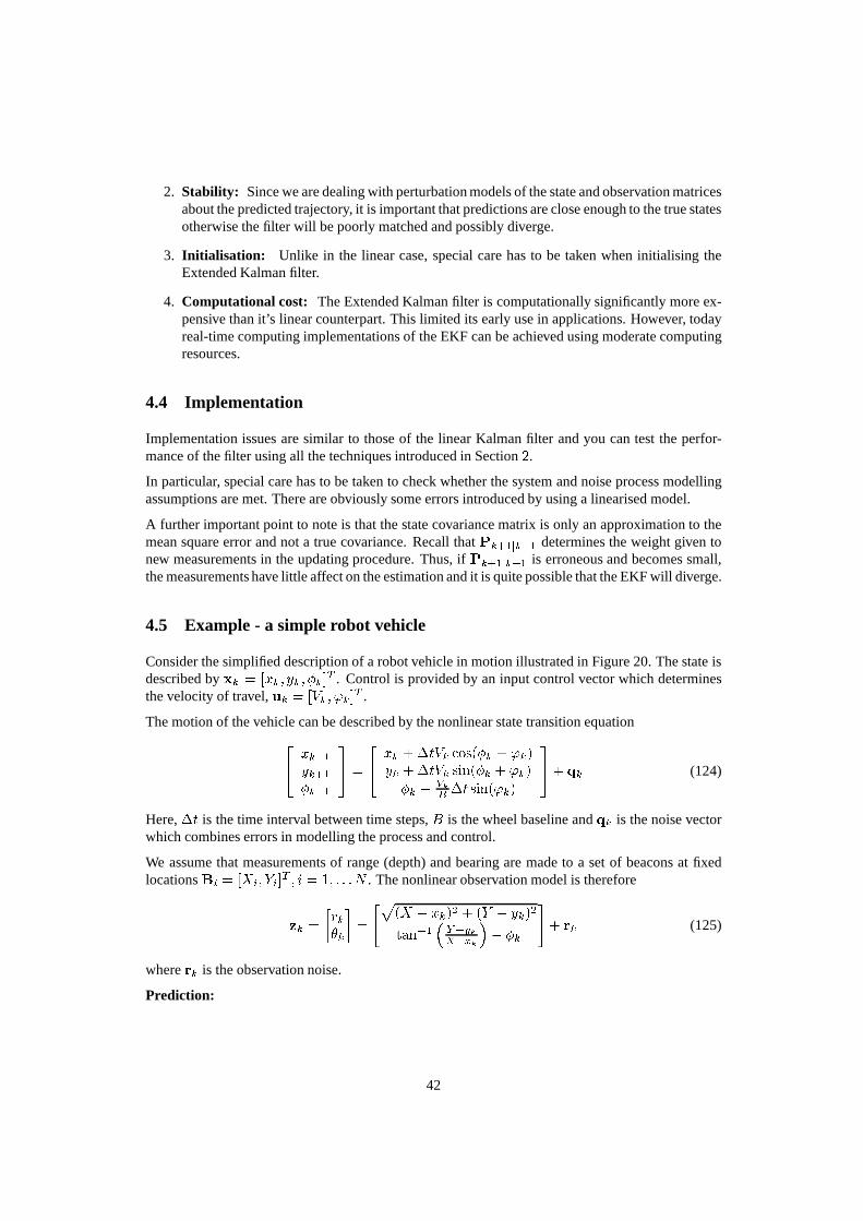
4.5 Example - a simple robot vehicle

Consider the simplified description of a robot vehicle in motion illustrated in Figure 20. The state isdescribed byxk = [xk; yk; �k℄T . Control is provided by an input control vector which determinesthe velocity of travel,uk = [Vk; 'k℄T .

The motion of the vehicle can be described by the nonlinear state transition equation24 xk+1yk+1�k+1 35 = 24 xk +�tVk os(�k + 'k)yk +�tVk sin(�k + 'k)�k + VkB �t sin('k) 35+ qk (124)

Here,�t is the time interval between time steps,B is the wheel baseline andqk is the noise vectorwhich combines errors in modelling the process and control.

We assume that measurements of range (depth) and bearing aremade to a set of beacons at fixedlocationsBi = [Xi; Yi℄T ; i = 1; : : :N . The nonlinear observation model is thereforezk = �rk�k� = "p(X � xk)2 + (Y � yk)2tan�1 � Y�ykX�xk �� �k #+ rk (125)

whererk is the observation noise.

Prediction:

42

y

xorigin

Bi

z(k)=(r,θ)

x(k)=(x,y,θ)T

γ

θ

Figure 20:Example: geometry of a simple robot vehicle.

From equation 109 the predicted statexk+1jk is given by24 xk+1jkyk+1jk�k+1jk 35 = 24 xkjk +�tVk os(�kjk + 'k)ykjk +�tVk sin(�kjk + 'k)�kjk + VkB �t sin('k) 35+ qk (126)

The prediction covariance matrix isPk+1jk = � �f�x�Pkjk � �f�x�T +Qk (127)

where � �f�x� = 24 1 0 ��tVk sin(�kjk + 'k)0 1 +�tVk os(�kjk + 'k)0 0 1 35 (128)

Update:

The equations for the updating of the state and its covariance are:xk+1jk+1 = xk+1jk +Kk+1[zk � h(xk+1jk)℄Pk+1jk+1 = Pk+1jk �Kk+1Sk+1KTk+1 (129)

where Kk+1 = Pk+1jk ��h�x�T S�1k+1 (130)

43

and Sk+1 = ��h�x�Pk+1jk ��h�x�T +Rk+1 (131)

and ��h�x� = " xk+1jk�Xd yk+1jk�Yd 0� yk+1jk�Yd2 xk+1jk�Xd2 �1 # (132)

Hered =p(X � xk+1jk)2 + (Y � yk+1jk)2.4.6 Measurement Validation - coping with Non-Gaussian Noise

Recall that in the first part of the course we considered the problem ofvalidating new measure-ments. Such considerations are particularly important in applications such as sonar tracking wheremeasurement ‘outliers’ are common; i.e. the sensor distribution (conditioned on the true value) is nolonger Gaussian.

The solution to this problem we developed was to set up avalidation gateor innovation gate; anymeasurement lying in the “region” of space defined by the gateis considered to be associated withthe target. Note that since the measurement vector typically has a number of components (say N) the“region” will be a region in N-dimensional space (typicallyan ellipsoid). We use the same approachwith the Kalman Filter and recap it here.

Assume that we already have a predicted measurementzk+1jk, hence theinnovation, �k+1 and itsassociated covarianceSk+1. Under the assumption that the innovation is normally distributed, thenormalised innovation�k+1S�1k+1�Tk+1 is distributed as a�2 distribution onn degrees of freedom,wheren is the dimension of the vector�.

Hence, as we saw in the first part of the course, we can define a confidence region (which we callhere the validation gate) such thatR( ) = fzj(zk+1 � zk+1jk)TS�1k+1(zk+1 � zk+1jk) � g= fzj�Tk+1S�1k+1�k+1 � g (133)

where can be obtained from standard�2 distribution tables.

In the context of the Kalman Filter algorithm, Equation 133 constrains the region of space where welook for a measurement. We assume that the correct measurement will be detected in this region. Itis possible, however, that more than one measurement will bein the valid region. The problem ofdistinguishing between the correct measurement and measurements arising from background clutterand other targets (false alarms) is calleddata association. This topic falls outside of the scope ofthe course (see, for example, Bar-Shalom and Fortmann).

44