1 Endogeneity

1. Formally, the problem is that, in a model

Y = g(X;�) + ";

the disturbances are endogenous, or equivalently, correlated with the re-gressors, as in

E[X 0"] 6= 0

In the Venn Diagram (Ballentine) on page 167 of Kennedy, we get a pictureof this. There is a variable X which does covary with Y (red+blue+purple),but sadly some of the covariance with Y is through covariance with theerror term (red). This covariance leads to bias in the OLS estimator.

2. Why do you get bias?

(a) Covariation of Y with the disturbance term, which is correlated withX, is attributed to X. Consider the case where

Y = X� + "; " = X� + � , Y = X (� + �) + �:

(b) The regression loads the response of Y to X entirely on to X. But inreality, the response of Y to X has two channels: the direct channelthrough �, and the indirect channel through �. The indirect channelis through the disturbance term: it is the derivative of " with respectto X.

(c) Think of the simplest possible regression model, where X is a uni-variate continuous variable in [�1; 1] and the true coe¢ cient is 1, butwhere

E[X 0"] = 1:

Here, X is positively correlated with the disturbance, which has ex-pectation 1 when X = 1, and expectation �1 when X = �1. Drawthe picture and you will see that the OLS estimator gives you thewrong slope. The reason is that it assigns variation that is due to thecovariance of X and the disturbance to covariation between X andY . Here, it will give you an estimate of 2 rather than 1.

(d) The covariance between X and the disturbance pollutes the OLS es-timator with variation that violates its identifying assumptions.

3. What causes endogeneity?

(a) Nothing need cause endogeneity. It is just about covariances.

1

(b) Simultaneity : Equations are said to be simultaneous if stu¤ on theRHS in one equation shows up in the LHS in other equation(s). Forexample, if

Y = X� + ";

X = Y �+ Z�;

then, substituting into X yields

X = X��+ Z� + "�

X �X�� = Z� + "�

X = [I � ��]�1 (Z� + "�) ;

which is obviously correlated with ". A classic reason that this couldhappen is if an underlying cause of the error term in your primaryequation is also an underlying cause of variation in one of the X�s.

(c) Correlated Missing Variables. If the true model is

Y = X� + Z� + ";

E�[X Z]

0"�= 0

but we estimate a model based on

Y = X� + ";

then, the expectation of the OLS estimator is

Eh�OLS

i= E

h(X 0X)

�1X 0 (X� + Z� + ")

i= � + E

h(X 0X)

�1X 0 (Z� + ")

i= � + (X 0X)

�1X 0Z� + (X 0X)

�1E [X 0"]

= � + (X 0X)�1X 0Z�

Here, even though the " are exogenous to the X�s, there is a biasterm depending on the empirical covariance between X and Z: IfX 0Z = 0, then �OLS is unbiased. If Z is a random variable, thenif E [X 0Z] = 0, then �OLS is unbiased: This is why only correlatedmissing variables are a problem: uncorrelated missing variables donot induce bias.

i. If X and Z are correlated, then the OLS estimator is comprisedof two terms added together: (1) the true coe¢ cient on X, and(2) the marginal e¤ect of X on Z�. The latter e¤ect maybe interpreted as � times the regression coe¢ cients on X in aregression of Z on X.

2

(d) Consider the model of earnings Y given characteristics X and school-ing levels W . Let � be a measure of smartness that a¤ects schoolingchoice. In a model like this, schooling will be correlated with thedisturbance because smart people both get more schooling and getmore money given schooling. Thus, the OLS estimate of the returnto schooling is biased upwards:

Y = X� +W� + "

whereW = Z + �

and the two disturbances are correlated, implying

E[�"] 6= 0

Here W is correlated with the disturbance ", which captures amongother things the impact of smartness on income conditional on school-ing.

(e) Selection Bias. Classic selection bias is when your sample selec-tion has di¤erent characteristics from the population in a way thatmatters for the coe¢ cient you are estimating. Eg, leaving out non-workers leaves out those who get no return to schooling. Formally,the problem is that the same thing that causes selection into thesampleXan observed wageXis correlated with having a higher valueof the disturbance term.

4. Corrections for endogeneity bias are always going to lie in dealing with thispollution by either (1) removing it; (2) controlling for it; or (3) modellingit.

2 Dealing With Endogeneity

1. how do you solve an endogeneity problem?

(a) Go back to the Venn Diagram. The problem is that we have red vari-ation that OLS mistakenly attaches to X. Three general approachesare

i. Clever Sample Selection. Drop the polluted observations of Xthat covary with the disturbance;

ii. Instrumental Variables or Control Variables. In each observa-tion, drop the polluted component of X or control for the pol-luted component of X.

iii. Full Information Methods. Model the covariation of errors acrossthe equations.

3

(b) Clever Sample Selection. Okay, so some of our observations havecovariance of X and the disturbances. But, maybe some don�t.

i. In the returns to schooling example, if some people, for examplethe very tall, were not allowed to choose their schooling level,but rather were just assigned an amount of time in school, thentheir W would be exogenous.

ii. Run a regression on the very tall only. You would have to assumethat their returns to schooling are the same as everyone else�sthough.

iii. If you are interested, for example, in the wage loss due to layo¤,you might worry that �rms layo¤big losers, so that layo¤ (on theRHS) is correlated with the disturbance in the pre-layo¤ wage.

iv. When �rms close entire plants, they don�t pick and choose whoto layo¤.

v. run a regression on people who were laid o¤ due to plant closuresonly.

(c) Instrumental Variables.

i. Say you have a variable, called an instrument, usually labelledZ, that is correlated with the polluted X, but not correlated withthe disturbance term. You could use that information instead ofX. This is the purple area in the Venn Diagram.

ii. The purple area is not correlated with the disturbance term byconstruction. Thus, you can use it in an OLS regression.

iii. The only problem is a regression of Y on the instrument givesyou the marginal impact of the instrument on Y , when you reallywanted the marginal impact of X on Y . You can solve this byexpressing the instrument in units of X. This is the spirit of twostage least squares.

iv. It is important to assess the strength of the instrument. Afterall, identi�cation and precision is coming from the covariation ofthe instrument with X and Y . If there isn�t much of this jointcovariation, you won�t get much precision. You will also get biasif the model is overidenti�ed. These problems are called WeakInstruments problems.

2. Two Stage Least Squares

(a) �nd an instrument Z such that

E[X 0Z] 6= 0; E[Z 0"] = 0;

and then use Z variation instead of X variation. The trick is to useZ variation which is correlated with X variation to learn about themarginal e¤ect of X on Y .

4

(b) Denote bX as the predicted values from a regression of X on Z. SinceZ is assume uncorrelated with the disturbances, bX must also beuncorrelated with the disturbances. Run a regression of Y on bX.This regression will satisfy the conditions which make OLS unbiased.This regression uses only the purple area in the Venn Diagram toidentify the marginal e¤ect of X on Y . Here,

�2SLS =� bX 0 bX��1 bX 0Y

where bX = Z (Z 0Z)�1Z 0X:

(c) Since, bX is a constructed variable, the output from this OLS regres-sion will give the wrong covariance matrix for the coe¢ cients. Thereason is that what you want is

b�2 � bX 0 bX��1where

b�2 = �Y �X�2SLS�0 �Y �X�2SLS� = (N �K)

This is because the estimate of the disturbance is still

e = Y �X�2SLS

even though the coe¢ cients are the IV coe¢ cients. But what you�dget as output is bs2 � bX 0 bX��1where

bs2 = �Y � bX�2SLS�0 �Y � bX�2SLS� = (N �K)

which is not the estimated variance of the disturbance.

3. Exactly Identi�ed (and homoskedastic) Case: Method of Moments Esti-mator:

(a) Recall: a method-of-moments approach substitutes sample analogsinto theoretical moments:

i. a moment is an expectation of a power of a random variable.ii. sample analogs are observed variables that can be plugged in.

5

iii. For example, given the assumption that

E[X 0"] = 0;

the method-of-moments approach to estimating parameters is tosubstitute sample moments into the restriction:

X 0e = 0, X 0(Y �X�) = 0:

The unique solution to this equation is the OLS estimate.iv. The method-of-moments approach tells you that the covariance

assumption onX and the disturbances is extremely closely linkedto the solution of minimising vertical distances.me

(b) De�nition: Projection Matrix

i. For any variable W , denote the projection matrix

PW �W (W 0W )�1W 0;

and note that in OLS, we may express predicted values in termsof this projection matrix as

Y = X� = X(X 0X)�1X 0Y = PXY

ii. projection matrices are idempotent: they equal their own square:

PWPW = PW :

iii. projection matrice are symmetric, so that PW = P 0W .iv. projection matrices have rank T where T is the rank of W .

(c) You can think about Two Stage Least Squares in a method-of-momentsway, too. The moment restrictions are

E[Z 0"] = 0

If Z is full rank with K columns, then we say that the model isexactly identi�ed. Substituting in sample moments yields

Z 0�Y �X�MoM

�= 0

Solving this for the coe¢ cients yields:

b�MoM = (Z 0X)�1Z 0Y

This is sometimes referred to as Indirect Least Squares.

6

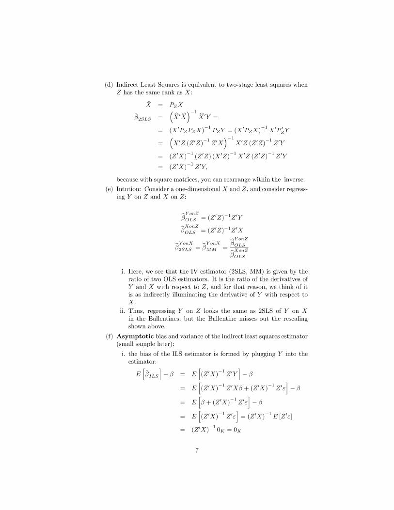
(d) Indirect Least Squares is equivalent to two-stage least squares whenZ has the same rank as X:

X = PZX

�2SLS =� bX 0 bX��1 bX 0Y =

= (X 0PZPZX)�1PZY = (X

0PZX)�1X 0P 0ZY

=�X 0Z (Z 0Z)

�1Z 0X

��1X 0Z (Z 0Z)

�1Z 0Y

= (Z 0X)�1(Z 0Z) (X 0Z)

�1X 0Z (Z 0Z)

�1Z 0Y

= (Z 0X)�1Z 0Y;

because with square matrices, you can rearrange within the inverse.

(e) Intution: Consider a one-dimensional X and Z, and consider regress-ing Y on Z and X on Z:

b�Y onZOLS = (Z 0Z)�1Z 0Yb�XonZOLS = (Z 0Z)�1Z 0X

b�Y onX2SLS = b�Y onXMM =b�Y onZOLSb�XonZOLS

i. Here, we see that the IV estimator (2SLS, MM) is given by theratio of two OLS estimators. It is the ratio of the derivatives ofY and X with respect to Z, and for that reason, we think of itis as indirectly illuminating the derivative of Y with respect toX.

ii. Thus, regressing Y on Z looks the same as 2SLS of Y on Xin the Ballentines, but the Ballentine misses out the rescalingshown above.

(f) Asymptotic bias and variance of the indirect least squares estimator(small sample later):

i. the bias of the ILS estimator is formed by plugging Y into theestimator:

Eh�ILS

i� � = E

h(Z 0X)

�1Z 0Y

i� �

= Eh(Z 0X)

�1Z 0X� + (Z 0X)

�1Z 0"

i� �

= Eh� + (Z 0X)

�1Z 0"

i� �

= Eh(Z 0X)

�1Z 0"

i= (Z 0X)

�1E [Z 0"]

= (Z 0X)�10K = 0K

7

ii. since the ILS estimator is asymptotically unbiased, aka, con-sistent, the variance is formed by squaring the term inside theexpectation in the bias expression:

E

���ILS � �

���ILS � �

�0�= E

h(Z 0X)

�1Z 0""0Z (Z 0X)

�1i:

Here, we need to assume something about E[""0] to make progress(just as in the OLS case). So, use the usual homoskedasticityassumption:

E[""0] = �2IN ;

so,

E

���ILS � �

���ILS � �

�0�= E

h(Z 0X)

�1Z 0""0Z (Z 0X)

�1i

= (Z 0X)�1Z 0�2INZ (Z

0X)�1

= �2 (Z 0X)�1Z 0Z (Z 0X)

�1:

If Z = X, then we have the OLS variance matrix.iii. This variance is similar to

V (")

Cov(X;Z)

V (Z)

Cov(X;Z);

so, to get precise estimates, you keep the variance of the dis-turbance V (") low, and the covariance between instruments andregressors Cov(X;Z) high. The right-hand term is the recipro-cal of the share of the variance of Z that shows up in X. If youget a big share of X in Z, the variance of the estimate is smaller.

4. Overidenti�ed (and homoskedastic) Case: Generalised Method of MomentsEstimator

(a) If Z contains more columns than X, we say that the model is overi-denti�ed. In this case, you have too much information, and you can�tget the moment restriction all the way to zero. Instead, you solvefor the coe¢ cients by minimising a quadratic form of the momentrestriction. This is called Generalised Method-of-Moments (GMM).The GMM estimator is exactly equal to the two stage least squaresestimator in linear homoskedastic models.

(b) Assume Z has J > K columns. GMM (Hansen 1982) proposesa criterion "get Z 0e as close to zero as you can by choice of theparameter vector �". Since � only has K elements and Z 0e hasmore than K elements, you can�t generally get Z 0e all the way tozero. So, you minimize a quadratic form in Z 0e with some kind ofweighting matrix in the middle. Consider

min�e0Z�1Z 0e

8

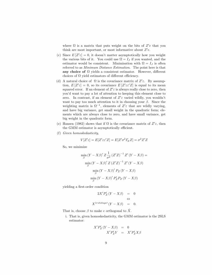
where is a matrix that puts weight on the bits of Z 0e that youthink are most important, or most informative about Z 0e.

(c) Since E [Z 0"] = 0, it doesn�t matter asymptotically how you weightthe various bits of it. You could use = IJ if you wanted, and theestimator would be consistent. Minimisation with = IJ is oftenreferred to as Minimum Distance Estimation. The point here is thatany choice of yields a consistent estimator. However, di¤erentchoices of yield estimators of di¤erent e¢ ciency.

(d) A natural choice of is the covariance matrix of Z 0". By assump-tion, E [Z 0"] = 0, so its covariance E [Z 0""0Z] is equal to its meansquared error. If an element of Z 0" is always really close to zero, thenyou�d want to pay a lot of attention to keeping this element close tozero. In contrast, if an element of Z 0" varied wildly, you wouldn�twant to pay too much attention to it in choosing your �. Since theweighting matrix is �1, elements of Z 0" that are wildly varying,and have big variance, get small weight in the quadratic form; ele-ments which are always close to zero, and have small variance, getbig weight in the quadratic form.

(e) Hansen (1982) shows that if is the covariance matrix of Z 0", thenthe GMM estimator is asymptotically e¢ cient.

(f) Given homoskedasticity,

V [Z 0"] = E[Z 0""0Z] = E[Z 0�2I 0NZ] = �2Z 0Z

So, we minimize

min�(Y �X�)0 Z 1

�2(Z 0Z)

�1Z 0 (Y �X�) =

min�(Y �X�)0 Z (Z 0Z)�1 Z 0 (Y �X�)

min�(Y �X�)0 PZ (Y �X�)

min�(Y �X�)0 P 0ZPZ (Y �X�)

yielding a �rst-order condition

2X 0P 0Z (Y �X�) = 0

,X1rststage0 (Y �X�) = 0:

That is, choose � to make e orthogonal to X.

i. That is, given homoskedasticity, the GMM estimator is the 2SLSestimator:

X 0P 0Z (Y �X�) = 0

X 0P 0ZY = X 0P 0ZX�

9

�GMM = �2SLS = (X0P 0ZX)

�1X 0P 0ZY

(g) Since all exogenous variables correspond to columns of X that arealso in Z, and de�ning as an instrument as an exogenous variablethat is in Z but not in X, this implies that you need at least oneinstrument in Z for every endogenous variable in X: Consider

X = [X1 X2]; Z = [X1 Z2];

a case where a subvector of X is exogenous (because it shows up inZ), and the rest is endogenous. Here, X2is endogenous.

Y = X� + " = X1�1 +X2�2 + "

The two stage approach to IV is to estimate X on Z and use itspredicted values on the RHS instead of X.What are its predicted values? Since Z contains the exogenous piecesof X, this is equivalent to regressing

Y = X1�1 + bX2�2 + "where bX2 = Z (Z 0Z)�1 Z 0

X2

the predicted values from a regression of the endogenous X�s on theentire set of Z.

i. What if X2contains interactions or squared terms, for example, ifschooling years are endogenous, then so, too, must be schoolingyears squared, and the interaction of schooling years with gender.So, even if the root is the endogeneity of schooling years, all theseother variables must be endogenous, too.

ii. In this case, two stage least squares must treat the endogenousvariables just as columns of X2. Thus, the bX2that gets used inthe �nal regession has the predicted value of schooling years and aseparate predicted value of schooling years squared. This lattervariable is not the square of the predicted value of schooling.You may wish to impose this restriction, but two stage leastsquares does not do it automatically. It is easy to see how toimpose it when using full information methods (below), but canbe cumbersome in limited information (IV and control variate)methods.

(h) The Asymptotic bias of this estimator is (small sample later)

Eh�2SLS

i� � = E

h(X 0P 0ZX)

�1X 0P 0ZY

i� �

= (X 0P 0ZX)�1X 0P 0ZX� + E

h(X 0P 0ZX)

�1X 0P 0Z"

i� �

= Eh(X 0P 0ZX)

�1X 0P 0Z"

i= (X 0P 0ZX)

�1X 0Z 0 (Z 0Z)

�1E [Z 0"] :

10

If Z is orthogonal to ", then this asymptotic bias is zero, so thatGMM/2SLS is consistent.

(i) The Asymptotic variance of the estimator is the square of this ob-ject. If the " are homoskedastic, then

V��2SLS

�= �2 (X 0P 0ZX)

�1X 0P 0Z""PZX (X

0P 0ZX)�1

= �2 (X 0P 0ZX)�1X 0Z (Z 0Z)

�1Z 0Z (Z 0Z)

�1Z 0X (X 0P 0ZX)

�1

= �2 (X 0P 0ZX)�1X 0Z (Z 0Z)

�1Z 0X (X 0P 0ZX)

�1

= �2�X 0Z (Z 0Z)

�1Z 0X

��1X 0Z (Z 0Z)

�1Z 0X (X 0P 0ZX)

�1

= �2 (X 0P 0ZX)�1;

which is a reweighted version of the variance of the OLS estimator.

5. 2SLS small-sample bias and Weak Instruments (see Angrist and Pisschke,pg 170ish).

(a) 2SLS is biased but consistent.(b) Consider the model

Y = X� + "

E[X 0"] 6= 0

E[Z 0"] = 0

E[Z 0X] 6= 0

E[""0] = �2IN

where, X;Z; " are all random variables. And, additionally, let

X = Z� + u

withE (u0") 6= 0;

so that we have in mind that X has a part correlated with " givenby u, and a part uncorrelated with " given by Z�.

(c) The estimated coe¢ cient vector via GMM/2SLS isb� = b�2SLS = b�GMM = (X 0PZX)�1X 0PZY

(d) Its bias is

Eh�2SLS

i� � = E

h(XPZX)

�1X 0PZ"

i:

Notice that the expectation is now over X and over the inverse. Itturns out that expectations of matrix inverses times other matricesare pretty close to the product of the two expectations, so that

Eh�2SLS

i� � � E

h(XPZX)

�1iE [X 0PZ"] :

11

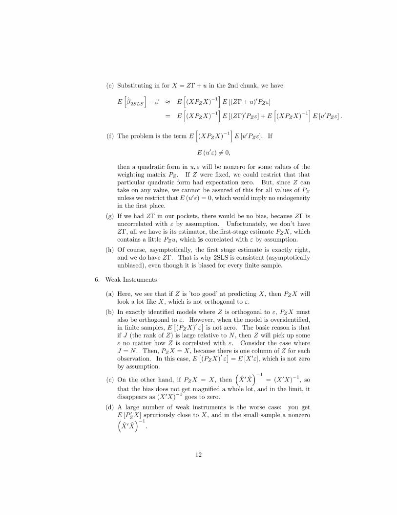
(e) Substituting in for X = Z� + u in the 2nd chunk, we have

Eh�2SLS

i� � � E

h(XPZX)

�1iE [(Z� + u)0PZ"]

= Eh(XPZX)

�1iE [(Z�)0PZ"] + E

h(XPZX)

�1iE [u0PZ"] :

(f) The problem is the term Eh(XPZX)

�1iE [u0PZ"]. If

E (u0") 6= 0;

then a quadratic form in u; " will be nonzero for some values of theweighting matrix PZ . If Z were �xed, we could restrict that thatparticular quadratic form had expectation zero. But, since Z cantake on any value, we cannot be assured of this for all values of PZunless we restrict that E (u0") = 0, which would imply no endogeneityin the �rst place.

(g) If we had Z� in our pockets, there would be no bias, because Z� isuncorrelated with " by assumption. Unfortunately, we don�t haveZ�, all we have is its estimator, the �rst-stage estimate PZX, whichcontains a little PZu, which is correlated with " by assumption.

(h) Of course, asymptotically, the �rst stage estimate is exactly right,and we do have Z�. That is why 2SLS is consistent (asymptoticallyunbiased), even though it is biased for every �nite sample.

6. Weak Instruments

(a) Here, we see that if Z is �too good�at predicting X, then PZX willlook a lot like X, which is not orthogonal to ".

(b) In exactly identi�ed models where Z is orthogonal to ", PZX mustalso be orthogonal to ". However, when the model is overidenti�ed,in �nite samples, E

�(PZX)

0"�is not zero. The basic reason is that

if J (the rank of Z) is large relative to N , then Z will pick up some" no matter how Z is correlated with ". Consider the case whereJ = N . Then, PZX = X, because there is one column of Z for eachobservation. In this case, E

�(PZX)

0"�= E [X 0"], which is not zero

by assumption.

(c) On the other hand, if PZX = X, then�X 0X

��1= (X 0X)

�1, so

that the bias does not get magni�ed a whole lot, and in the limit, itdisappears as (X 0X)

�1 goes to zero.

(d) A large number of weak instruments is the worse case: you getE [P 0ZX] spruriously close to X, and in the small sample a nonzero�X 0X

��1.

12

(e) If you have lots of overidenti�cation, then even with homoskedastic-ity, the term P 0Z""PZ will not have expectation �

2PZ in the smallsample. Thus, when you have overidenti�cation and weak instru-ments, you get both bias and weird standard errors.

(f) What if your instruments are only weakly correlated with X. This isthe problem of weak instruments (see the suggested reading). Weakinstruments are an issue in overidenti�ed models where the instru-ments are only weakly correlated with the endogenous regressor(s).In this case, you have small-sample bias, and high variance at anysample size.

(g) This problem goes away asymptotically, but if you have crappy enoughinstruments with weak enough correlation with X, you can induce ahuge small sample bias even if the instruments are truly exogenous.

(h) We can approximate the small-sample bias. Hahn and Hausman(2005), who explore the case with 1 endogenous regressor, write the(second-order) approximation of the small-sample bias of the 2SLSestimator for that endogenous regressor proportional to

Eh�2SLS

i� � _

L��1� ~R2

�N ~R2

;

where ~R2 is the R2 value in the �rst-stage regression, J is the numberof instruments, � is the correlation between the endogenous regressorand the model disturbance term, and N is the sample size.

i. Obviously, this goes to zero as N goes to 1, so the the 2SLSestimator is consistent.

ii. However, if the instruments are weak, so that ~R2 is small, thebias gets large.

iii. Further, if the model is highly overidenti�ed, so that J is verylarge, the bias gets large.

iv. the correlation � is the reason that there is an endogeneity prob-lem in the �rst place. Indeed, the bias of the OLS regressioncoe¢ cient is proportional to �.

v. We may rewrite this expression in terms of the �rst stage Fstatistic, too:

Eh�2SLS

i� � � �u"

�21

F + 1;

(i) one can express the bias of the 2SLS estimator in terms of the biasof the OLS estimator:

Biash�2SLS

i=

J

N ~R2Bias

h�OLS

i;

13

so if J > N ~R2, 2SLS is certainly worse than OLS: it would havebigger bias and, as always, it would have bigger variance. Of course,even if 2SLS has smaller bias, it may enough more variance that it isstill undesirable in Mean Squared Error terms.

(j) A simple comparison of J to N ~R2 gives you a sense of how big the2SLS bias is. Since that fraction is strictly positive, 2SLS is biasedin the same direction as OLS, so if you have theory for the directionof OLS bias, the same theory works for 2SLS bias.

7. Rules of Thumb

(a) Report the �rst stage and think about whether it makes sense. Arethe magnitude and sign as you would expect, or are the estimatestoo big or large but wrong-signed? If so, perhaps your hypothesized�rst-stage mechanism isn�t really there, rather, you simply got lucky.

(b) Report the F-statistic on the excluded instruments. The bigger thisis, the better. Stock, Wright, and Yogo (2002) suggest that F-statistics above about 10 put you in the safe zone though obviouslythis cannot be a theorem.

(c) Pick your best single instrument and report just-identifed estimatesusing this one only. Just-identifed IV is approximately unbiased andtherefore unlikely to be subject to a weak-instruments critique.

(d) Check over-identifed 2SLS estimates with LIML. LIML is less precisethan 2SLS but also less biased. If the results come out similar, behappy. If not, worry, and try to �nd stronger instruments.

(e) Look at the coe¢ cients, t-statistics, and F-statistics for excludedinstruments in the reduced-form regression of dependent variableson instruments. Remember that the reduced form is proportionalto the causal e¤ect of interest. Most importantly, the reduced-formestimates, since they are OLS, are unbiased. Angrist and Krueger(2001), and many others, believe that if you can�t see the causalrelation of interest in the reduced form, it�s probably not there.

8. GMM in non-homoskedastic and nonlinear models.

(a) If the disturbances are not homoskedastic and the model is overiden-ti�ed (Z has higher rank than X), then GMM is not equivalent to2SLS. GMM would give di¤erent numbers.

(b) Here, the key is to get an estimate of , given by . Any consistentestimate of will do the trick. How big is ? It is the covariancematrix of Z 0", so it is a symmetric JxJ matrix, with J(J + 1)=2distinct elements. Note that this number does not grow with N .

14

(c) Recall that GMM is consistent regardless of which is used. Thus,one can implement GMM with any old (such as the 2SLS estima-tor), collect the residuals, e, and construct

=1

N

X(Z 0ee0Z) ;

and then implement GMM via

min�e0Z�1Z 0e

(d) GMM can be used in nonlinear models, too. Consider a model

Y = f(X;�) + "

The moment restrictions are

E[Z 0"] = 0

Substituting in sample moments yields

Z 0 (Y � f(X;�)) = 0:

Thinking in a GMM way, it is clear that if the rank of Z is less thanthe length of �, you won�t have enough information to identify �.This is equivalent to say (in full-rank linear models) that you needat least one column of Z for each column of X.

(e) If J > K, you can�t get these moments all the way to zero, so onewould minimize

0min�(Y � f(X;�))0 Z�1Z 0 (Y � f(X;�))

where is an estimate of the variance of the moment conditions.

9. Are the Instruments Exogenous? Are the Regressors Endogeneous?

(a) If the regressors are endogeneous, then the OLS estimates shoulddi¤er from the endogeneity-corrected estimates (as long as the in-struments are exogenous).

(b) The test of this hypothesis is called a Hausman Test.

(c) If the instruments are exogenous and you have an overidenti�edmodel, then you can test the exogeneity of the instruments.

(d) Under the assumption that at least one instrument is exogenous, youcan test whether or not all the instruments are exogenous.

(e) Test of Overidentifying Restrictions

15

(f) Under the assumption that all the instruments are exogenous, wehave from the model that

E [Z 0"] = 0

E [Z 0""0Z] = :

(g) The GMM estimator, minimised a quadratic form of Z 0e:

minb� e0Z�1Z 0e;

where = E [Z 0""0Z] is the (possibly estimated) covariance matrixof Z 0".

(h) If we had observed ", we might have considered the optimisation

minb� "0Z�1Z 0";

and, so, if we premultiplied everything by �1=2, we�d have

Eh�1=2Z 0"

i= 0;

E�"0Z�1Z 0"

�= IJ ;

so the quadratic form would be the square of a bunch of mean-zero,unit variance, uncorrelated random variables.

(i) If the model is homoskedastic, then �1 = 1�2 (Z

0Z)�1, so you don�t

even need to know . You�d have

minb�1

�2"0Z (Z 0Z)

�1Z 0" = minb�

1

�2"0PZ" = minb�

1

�2"0PZP

0Z"

and, so, if we premultiplied everything by �1=2, we�d have

E [P 0Z"] = 0;

E ["0PZP0Z"] = IJ :

(j) But, e isn�t ". The residual is related to the model via:

e = (Y �Xb�)= (Y �X 0 (X 0P 0ZX)

�1X 0P 0ZY )

=hI �X 0 (X 0P 0ZX)

�1X 0P 0Z

iY

=hI �X 0 (X 0P 0ZX)

�1X 0P 0Z

i(X� + ")

=hX� �X 0 (X 0P 0ZX)

�1X 0P 0ZX�

i+hI �X 0 (X 0P 0ZX)

�1X 0P 0Z

i"

=hI �X 0 (X 0P 0ZX)

�1X 0P 0Z

i":

16

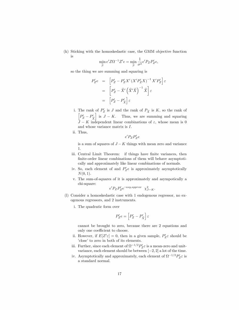
(k) Sticking with the homoskedastic case, the GMM objective functionis

minb� e0Z�1Z 0e = minb�1

�2e0PZP

0Ze;

so the thing we are summing and squaring is

P 0Ze =hP 0Z � P 0ZX 0 (X 0P 0ZX)

�1X 0P 0Z

i"

=

�P 0Z � bX 0

� bX 0 bX��1 bX� "=

hP 0Z � P 0bX

i"

i. The rank of P 0Z is J and the rank of P bX is K, so the rank ofhP 0Z � P 0bX

iis J � K. Thus, we are summing and squaring

J � K independent linear combinations of ", whose mean is 0and whose variance matrix is I.

ii. Thus,e0PZP

0Ze

is a sum of squares of J �K things with mean zero and variance1.

iii. Central Limit Theorem: if things have �nite variances, then�nite-order linear combinations of them will behave asymptoti-cally and approximately like linear combinations of normals.

iv. So, each element of and P 0Ze is approximately asymptoticallyN(0; 1).

v. The sum-of-squares of it is approximately and asympotically achi-square:

e0PZP0Ze~

asy;approx �2J�K :

(l) Consider a homoskedastic case with 1 endogenous regressor, no ex-ogenous regressors, and 2 instruments.

i. The quadratic form over

P 0Ze =hP 0Z � P 0bX

i"

cannot be brought to zero, because there are 2 equations andonly one coe¢ cient to choose.

ii. However, if E[Z 0"] = 0, then in a given sample, P 0Z" should be�close�to zero in both of its elements.

iii. Further, since each element of �1=2P 0Z" is a mean-zero and unit-variance, each element should be between [�2; 2] a lot of the time.

iv. Asymptotically and approximately, each element of �1=2P 0Z" isa standard normal.

17

v. But, the 2 elements of �1=2P 0Z" are linear in each other, so ifyou move one of them, you move the other by a �xed amount.

vi. Thus, the sum of squares of these is not the sum of 2 squarednormals, but just a single squared normal.

vii. So, if the GMM objective function is 50 at its minimum, thisnumber is too high to believe that you really had exogenousinstruments� more likely, you had an endogenous instrument.

10. What are good instruments?

(a) Going back to the Ballentine/Venn Diagrams in Kennedy, you wantan instrument Z that has no purple stu¤ in it (no correlation withthe disturbance terms),

E [Z 0"] = 0;

and which has lots of correlation with X,

E [Z 0X] 6= 0:

(b) What if you have instruments that violate this? Consider violationof exogeneity. In the linear exactly identi�ed case:

b�2SLS = b�(G)MM = (Z 0X)�1Z 0Y;

so, the bias term is

Ehb�2SLS � �i = E

�(Z 0X)�1Z 0Y � �

�= E

�(Z 0X)�1Z 0X� + (Z 0X)�1Z 0"� �

�= E

�(Z 0X)�1Z 0"

�= (Z 0X)�1E [Z 0"] ;

so, the degree to which E [Z 0"] is not zero gets reweighted by (Z 0X)�1

to form the bias. If E [Z 0"] is big, the bias is big, unless (Z 0X)�1

is really small. The matrix (Z 0X)�1 is small if Z 0X is big, which isthe case if Z and X covary a lot. Thus, even if your instrument isnot perfectly exogenous, you still want lots of correlation with X.

11. Control Variables

(a) Denote b� as the residuals from a regression of X on Z. The residual b�contains the same information about the endogeneity as bX. If bX is apart of X that is not polluted, then b� must contain all the pollution.

(b) That means that if we add b� to the RHS of the original speci�cation,it will control out the endogeneity.

18

(c) estimate by OLSY = X� + b� + "

The intuition is that b� is a control for the pollution in X. So, if X ispositively correlated with the disturbance, then

b�will be a big number when X is big, and small when X is small. Thispolluted covariation with Y will be assigned to b� (measured by ),and not to X.

(d) In linear homoskedastic models, the estimated coe¢ cients on X (andtheir variance) is the same whether you use GMM, 2SLS or controlvariables.

(e) The fact that the control variable comes in additively is important.It makes the whole system triangular, and therefore writeable in thisfashion. In nonlinear, semiparametric and nonparametric models,sometimes the control variable approach is easier, but it has to comein additively (Newey & Powell Econometrica 1997, 2003).

(f) Most everyone uses IV and not control variables.

12. Model the endogeneity (Full Information)

(a) Consider the two equation model

Yi = Xi� + "i

Xi = Zi� + �i

E["i�i] 6= 0:

Assume that Z has at least the rank of X, and that Z is exogenous.An example of this might be

Xi = [X1i X2i]; Zi = [X1i Z2i];

a case where a subvector of X is exogenous (because it shows up inZ), and the rest is endogenous.

(b) We could assume that�"i�i

�~N

��00

�;

��2" ��"�"�

��"�� �2�

��= N(02;�)

and estimate the parameters inside this normal, and the parametersof the two equations, by maximum likelihood. This would be called"full information maximum likelihood" (FIML).

19

(c) The FIML estimator would use the fact that

��1=2�"i�i

�~N

��00

�;

�1 00 1

��= N(02; I2)

where

��1=2 =

��2" ��"�"�

��"�� �2�

��1=2:

(d) Let � e"ie�i�= ��1=2

�"i�i

�:

Then, the density of observation i is

� (e"i)� (e�i)and the likelihood to be maximized by choice of �;�; �2"; �

2�; � is

max�;�;�2";�

2�;�lnL =

NXi=1

ln��e"i(Yi; Xi;�;�; �2"; �2�; �)�+ln� �e�i(Yi; Xi;�;�; �2"; �2�; �)�

(e) Note that for a mean-zero bivariate normal, the conditional distribu-tion (http://en.wikipedia.org/wiki/Multivariate_normal_distribution#Conditional_distributions)of one given the other is

"ij�i=�~N(�"����; (1� �2)�2"):

This conditional distribution is not mean-zero. Indeed, its mean islinear in �:

(f) If you just regress Y on X, the expectation of "i is �"����i. That is

the bias term in the endogenous regression. It is zero if and only if� = 0.

(g) Consider adding �i as a regressor. Its coe¢ cient in the regressionwould be �"

��� and it would soak up all the endogeneity.

(h) Thus, a control function approach to this ML problem would be toregress X on Z, collect residuals ni = Xi � Zib�, and then regress Yon X and n.

(i) This is called "limited information maximum likelihood" (LIML) be-cause we don�t take all the information about the distribution of "igiven �i: Instead, we just try to control out is mean. We leave allthe other moments of that distribution unconstrained.

13. Selection-Corrections

20

(a) Consider the two equation model

Yi = Xi� + "i

Yi observed if Y � = Zi� + �i > 0;�"i�i

�~N

��00

�;

��2" ��"�"�

��"�� �2�

��Assume that Z has at least the rank of X, and that Z is exogenous.An example of this might be

Xi = [X1i X2i]; Zi = [X1i Z2i];

a case where a subvector of X is exogenous (because it shows up inZ), and the rest is endogenous.

(b) Here, Yi is observed only for some observations. For other observa-tions, we observe Z (which includes X) but not Y .

(c) Yi could be wages. Wages are only observed for workers, but labourforce attachment is observed for all people (be they workers or non-workers).

(d) Suppose that an unobservable, like ability, is correlated with bothlabour force attachment (the probability of working) and with wages.If ability were correlated with, e.g., an observable like education, thiswould induce endogeneity in the �rst equation above if we were tojust regress Y X. The reason is that the sample of workers withobserved wages would be richer with high-ability people than the fullpopulation of people which included nonworkers.

(e) The challenge is to �gure out the conditional expectation of "i forobservations with values of �i that put them into the category ofhaving observed Yi .

(f) Since the conditional distribution

"ij�i=�~N(�"����; (1� �2)�2");

the conditional mean is

E["ij�i=�] =�"����;

which is linear in �, so the mean of "i across all the values of �consistent with Y being observed is linear in the average value ofthose ��s.

(g) Consider the values of � consistent with Y being observed. For anyZi�, to get Y � > 0 we need �i > �Zi�. So we need the expectationof �i given that it lies above �Zi�.

21

(h) This expectation is called the "truncated mean" and the truncatedmean of a normal variate is easily looked up onWikipedia http://en.wikipedia.org/wiki/Truncated_normal_distribution.In our context, it is

E��ij�i>�Zi�

�= ���(

�Zi���

);

where

� (x) =�(x)

1� � (x)is the "Inverse Mills Ratio".

(i) Consequently,

E["ijYi observed ] =�"���E��ij�i>�Zi�

�= �"��(

�Zi���

):

This is the bias term in the regression of Y on X.

(j) So, a FIML approach would be analogous to that in 12 above. ALIML approach is very easy to implement via the 2-step "HeckmanRegression":

i. probit (Yi observed) on Ziii. predict �i, invmillsiii. regress Yi Xi �iiv. The coe¢ cient on �i goes to �"� and corrects for bias induced

by unobservables correlated with selection into the labour force.

22