1

Examining Relationships in Data

William P. Wattles, Ph.D.

Francis Marion University

12

Examining relationships

Correlational design- – observation only– look for relationship– does not imply cause

Experimental design- A study where the experimenter actively changes or manipulates one variable and looks for changes in another.

Dependent Variable

What we are trying to predict. It measures the outcome of a study.

Independent Variable

Is used to explain changes in the dependent variable

15

Correlation

The relationship between two variables X and Y.

In general, are changes in X associated with Changes in Y?

If so we say that X and Y covary. We can observe correlation by looking at a

scatter plot.

16

Psy 300 Exam one versus exam two

50%

55%

60%

65%

70%

75%

80%

85%

90%

95%

100%

50% 55% 60% 65% 70% 75% 80% 85% 90% 95% 100%

Grade on exam 2

Ex

am

3

17

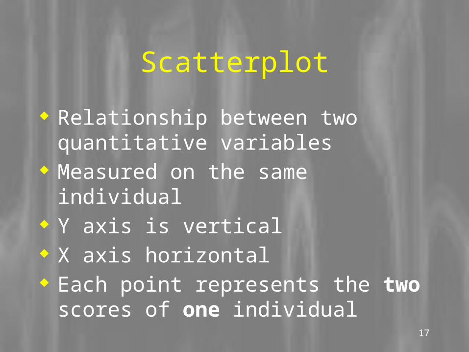
Scatterplot

Relationship between two quantitative variables

Measured on the same individual Y axis is vertical X axis horizontal Each point represents the two scores of one

individual

18

Type of correlation

Positive correlation. The two change in a similar direction. Individuals below average on X tend to be below average on Y and vice versa.

Negative correlation the two change in the opposite direction. Individuals who are above average on X tend to be below average on Y and vice versa.

Example of correlation from New York Times

Early studies have consistently shown that an "inverse association" exists between coffee consumption and risk for type 2 diabetes, Liu said. That is, the greater the consumption of coffee, the lesser the risk of diabetes

19

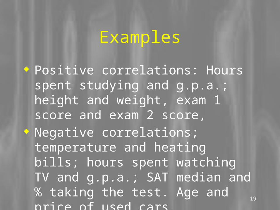
Examples

Positive correlations: Hours spent studying and g.p.a.; height and weight, exam 1 score and exam 2 score,

Negative correlations; temperature and heating bills; hours spent watching TV and g.p.a.; SAT median and % taking the test. Age and price of used cars.

20

Correlation Coefficient

One number that tells us about the strength and direction of the relationship between X and Y.

Has a value from -1.0 (perfect negative correlation) to +1.0 (perfect positive correlation)

Perfect correlations do not occur in nature

21

Correlation Coefficient

The Pearson Product Moment Correlation Coefficient or Pearson Correlation Coefficient is symbolized by r.

When you see r think relationship.

22

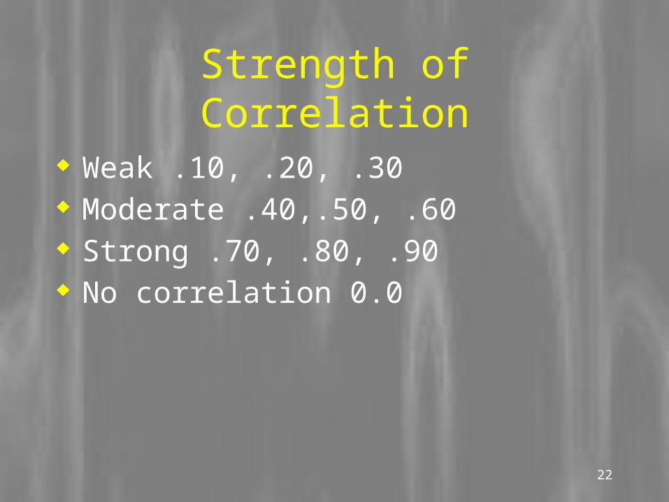
Strength of Correlation

Weak .10, .20, .30 Moderate .40,.50, .60 Strong .70, .80, .90 No correlation 0.0

23

Calculating a correlation coefficient

Deviation score for X (X-Xbar) Deviation score for Y (Y-Ybar) Standard deviations (SD) for X and Y Number of subjects (n)

24

Correlation Coefficient

rn

x x

s

y y

sx y

1

1( )( )

25

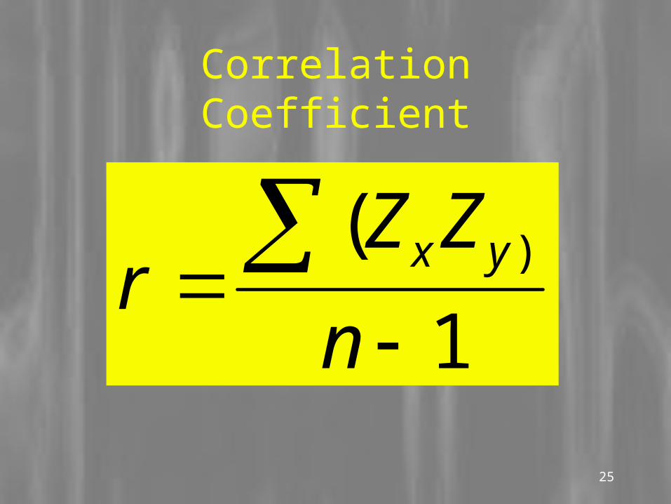
Correlation Coefficient

rZ Z

nx y

( )

1

26

Pearson Correlation Coefficient

Sum of (X-Xbar) times (Y-Ybar)/SD of X * SD of Y * n-1

A Pearson correlation coefficient does not measure non-linear relationships

We represent the Pearson correlation coefficient with r.

Student Number of Beers

Blood Alcohol Level

1 5 0.1

2 2 0.03

3 9 0.19

6 7 0.095

7 3 0.07

9 3 0.02

11 4 0.07

13 5 0.085

4 8 0.12

5 3 0.04

8 5 0.06

10 5 0.05

12 6 0.1

14 7 0.09

15 1 0.01

16 4 0.05

Here we have two quantitative

variables for each of 16 students.

1. How many beers they

drank, and

2. Their blood alcohol

level (BAC)

We are interested in the

relationship between the

two variables: How is one

affected by changes in the

other one?

Student Beers BAC

1 5 0.1

2 2 0.03

3 9 0.19

6 7 0.095

7 3 0.07

9 3 0.02

11 4 0.07

13 5 0.085

4 8 0.12

5 3 0.04

8 5 0.06

10 5 0.05

12 6 0.1

14 7 0.09

15 1 0.01

16 4 0.05

In a scatterplot one axis is used to represent

each of the variables, and the data are plotted as

points on the graph.

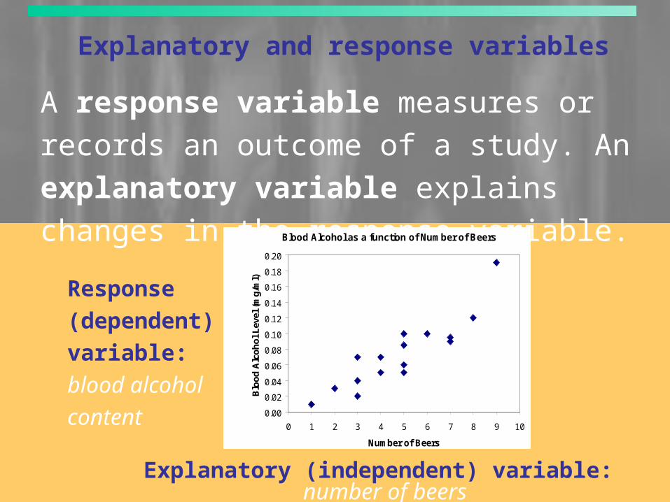
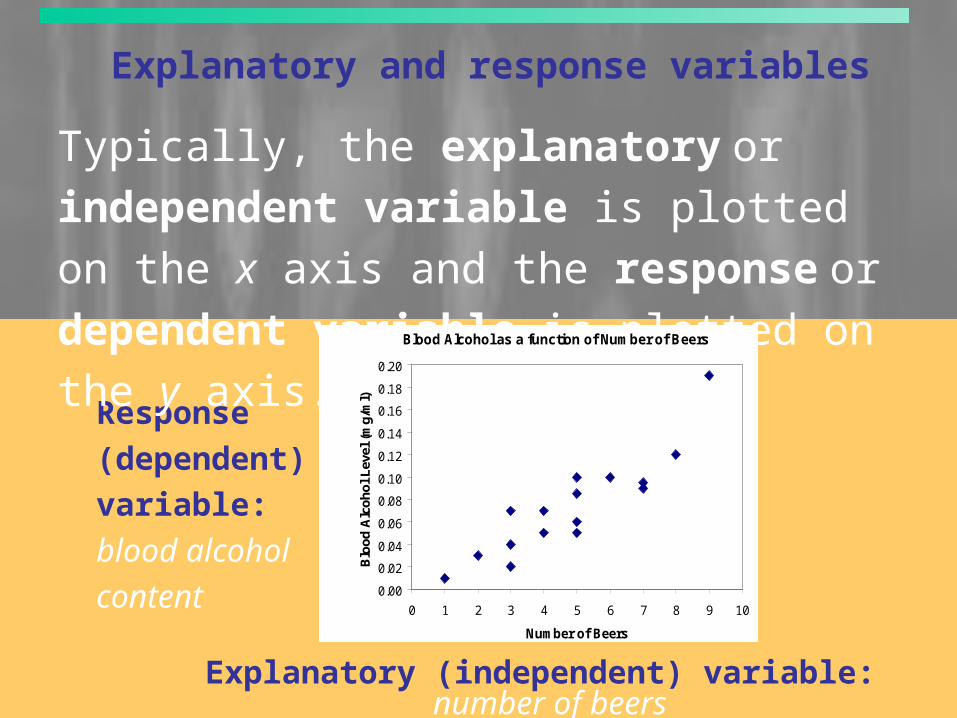
Explanatory (independent) variable: number of beers

Blood Alcohol as a function of Number of Beers

0.00

0.02

0.04

0.06

0.08

0.10

0.12

0.14

0.16

0.18

0.20

0 1 2 3 4 5 6 7 8 9 10

Number of Beers

Blo

od A

lcoh

ol L

evel

(m

g/m

l)Response

(dependent)

variable:

blood alcohol

contentx

y

Explanatory and response variables

A response variable measures or records an

outcome of a study. An explanatory variable

explains changes in the response variable.

Explanatory (independent) variable: number of beers

Blood Alcohol as a function of Number of Beers

0.00

0.02

0.04

0.06

0.08

0.10

0.12

0.14

0.16

0.18

0.20

0 1 2 3 4 5 6 7 8 9 10

Number of Beers

Blo

od A

lcoh

ol L

evel

(m

g/m

l)Response

(dependent)

variable:

blood alcohol

contentx

y

Explanatory and response variables

Typically, the explanatory or independent

variable is plotted on the x axis and the response

or dependent variable is plotted on the y axis.

27

Linear relationships

The Pearson correlation coefficient only works for linear relationships.

The assumption of linearity can be verified by examining a scatterplot.

Assumes that the relationship between X and Y is the same at different levels of X and Y

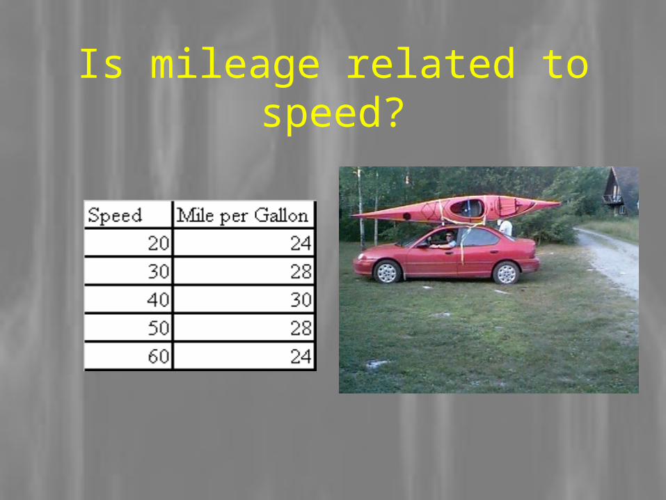
Is mileage related to speed?

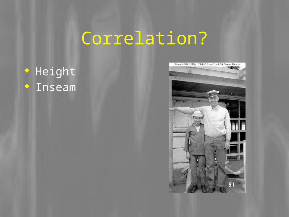
Correlation?

Height Inseam

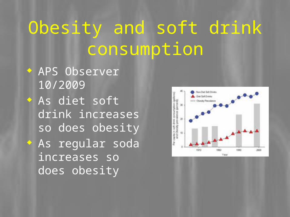
Obesity and soft drink consumption

APS Observer 10/2009

As diet soft drink increases so does obesity

As regular soda increases so does obesity

28

Correlation does not imply causation!

Correlation = .59

The End

3

What is a Z score?

4

What is the standard deviation?

5

What percentage of observations

lie within one standard

deviation of the mean?

6

What is the mean?

7

What is the formula for the standard deviation?

8

What percentage score less than a z-score of +1?

9

What is a Z-score?

10

What is the formula for a Z-score?

17/21= .81

4/21= .19 x 100= 19%

One number that tells about the variability in the sample or

population.

How many standard deviations an individual's

score lies above or below the mean.

68%

One number that tells us about the middle of the data,

using all the data.

sx x

n

( ) 2

1

84%

How many standard deviations a score lies above

or below the mean.

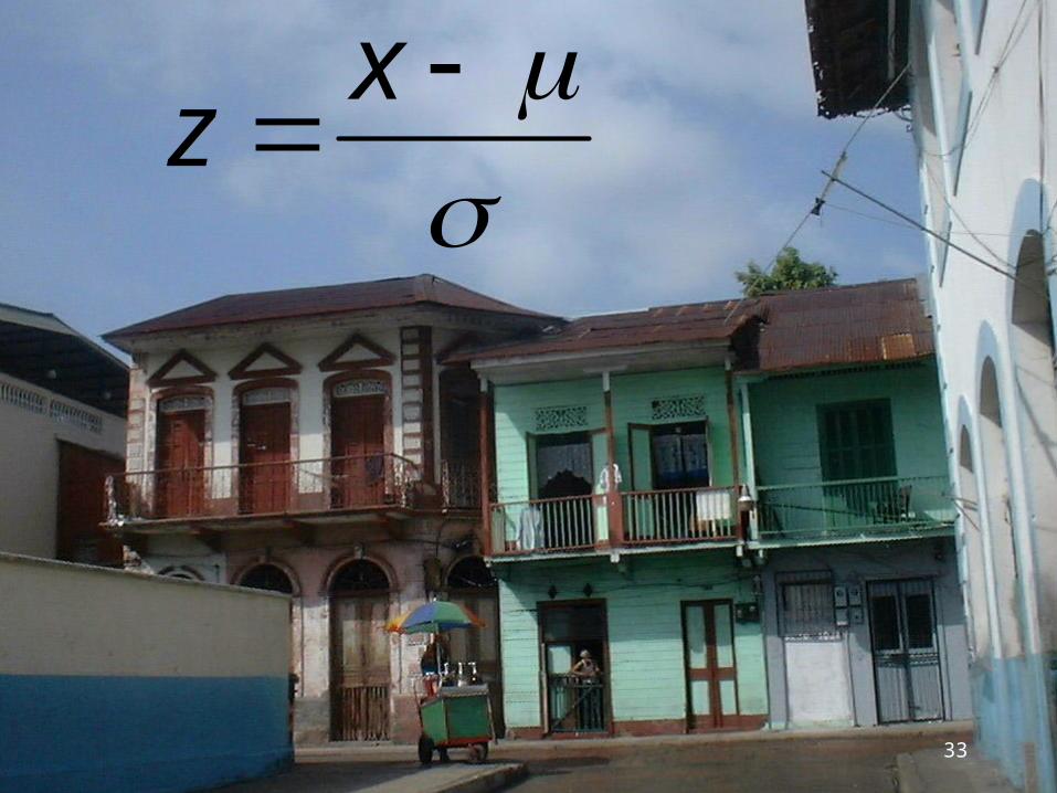
33

zx

The End

The End