1 game theoretic anti-jamming dynamic frequency hopping

1

Game Theoretic Anti-jamming DynamicFrequency Hopping and Rate Adaptation in

Wireless SystemsM. K. Hanawal, M. J. Abdel-Rahman, D. Nguyen, and M. Krunz

Department of Electrical and Computer EngineeringUniversity of Arizona, Tucson, AZ 85721, USA

{mhanawal, mjabdelrahman, dnnguyen, krunz} @email.arizona.eduTechnical Report

TR-UA-ECE-2013-3

Abstract

Wireless transmissions are inherently broadcast in nature and are vulnerable to jamming attacks.Frequency hopping (FH) and transmission rate adaptation (RA) have been used to mitigate jamming.However, recent works have shown that using either FH or RA (but not both) is inefficient against smartjamming. In this paper, we propose mitigating jamming by jointly optimizing the FH and RA techniques.We consider an average-power constrained “sweep” jammer that aims at degrading the goodput of awireless link. We model the interaction between the legitimate transmitter and jammer as a Markovzero-sum game, and derive optimal defense strategies against worst-case attack strategies. We comparethe average goodput and success rate under the new scheme with the schemes that rely on either FHor RA, but not both. Numerical investigations show that the new scheme improves the average goodputand provides better jamming resiliency.

Index Terms

Dynamic frequency hopping, jamming, Markov decision processes, Markov games, waveform adap-tation.

I. INTRODUCTION

The convenience of wireless communications and its support for mobility have increasedthe popularity of wireless devices. While wireless networks offer great flexibility, their openbroadcast nature leaves them vulnerable to various security threats, including jamming attacks. Ina jamming attack, an adversary injects interfering power into the wireless medium that can hinderlegitimate wireless communication in one of two ways: (i) the jamming power can degrade thesignal-to-interference-plus-noise ratio (SINR) at a legitimate receiver, and (ii) in carrier sensingnetworks, continuous jamming may prevent the legitimate transmitter from accessing the medium,hence, creating a denial-of-service attack. In this paper, we consider the attack of the first typeand develop optimal defense strategies against it. The open nature of the wireless medium makesit easy for an adversary to monitor communications between wireless devices and use readilyavailable off-the-shelf commercial products to launch a stealth jamming attacks [1], [2], [3].

Several physical-layer techniques have been developed to mitigate jamming, including spreadspectrum (e.g., frequency hopping), directional antennas, and power/coding/modulation control.Jammer-specific techniques have also been developed [1]. Common jamming models in the

August 26, 2013 DRAFT

2

literature include random jammer, constant jammer, proactive jammer, reactive jammer [2], [4],etc. This classification is based on the channel behavior and transmission capabilities of thejammer. Constant and proactive jammers always emit power into the medium. While a constantjammer transmits power at a fixed level all the time, a proactive jammer can vary the powerto meet various constraints. A reactive jammer exhibits more capabilities and emits power onlywhen he detects a legitimate transmission [3]. In this paper, we consider a proactive jammingattack in which the jammer jams one channel at a time and sweeps through all channels. Theprocess is repeated over and over again, but each time with a new (random) sweep pattern. Theamount of damage the jammer can inflict depends on his capabilities. Although transmittingcontinuously at the maximum power will enable the jammer to cause the maximum harm, thishappens at the cost of high energy consumption and, more importantly, a high likelihood ofbeing detected. In this work, we assume the jammer has a constraint on its average power.

Frequency hopping (FH) [5], [6] and rate adaption (RA) [7], [8] are commonly used techniquesto mitigate jamming. However, these techniques are shown to be ineffective when appliedseparately. In the case of RA with no FH, it is shown that by merely randomizing his power levelsthe jammer can force the transmitter to always operate at the lowest rate [9] if the jammingaverage power reaches a given threshold. This is captured through a zero-sum game whoseNash Equilibrium’s (NE) throughput is plotted in Figure 1(a). Experiments on IEEE 802.11networks with different RA schemes (e.g., SampleRate, ONOE) [10], [11] also confirm thisobservation. FH is shown to be largely inadequate in coping with jamming attacks in current802.11 networks [12]. In particular, when the number of channels is small and channels are notperfectly orthogonal, experimental studies in [12] show that the jammer can degrade the linkgoodput significantly.

Our aim in this paper is to study the effectiveness of a jointly optimized RA and FH techniqueto mitigate jamming. The potential of jointly optimizing the RA and FH to combat jammersis demonstrated in Figure 1. In this figure, we draw the NE’s throughput of the zero-sumgame between a jammer and a link that has freedom in selecting the transmission rate andhopping between channels. In this work, we will develop mechanisms that guide the link tomake instantaneous decision (i.e., pure strategy)[13] with or without complete information ofthe jammer.

In a multi-channel system, the transmitter can run away from the jammer by hopping fromone channel to another. But, hopping may result in loss of throughput as transmitter may notbe able to start transmission on the new channel instantaneously. Also, it cannot reside onthe same channel for longer time as the sweep jammer may reach that channel. In adoptingtransmission rates the transmitter faces similar dilemma; Using higher rate increases chances ofgetting jammed. On the other hand, if it uses lower rate, it will encounter a loss in throughput.We seek to derive jointly optimal dynamic frequency hopping and rate adaptation policies forthe transmitter against a proactive sweep jammer. This policy informs the transmitter when toswitch (hop) to another channel and when to continue (stay) on the current channel. Furthermore,it gives the best rate to use in both cases (hop and stay).

Main Contributions:• We model the interaction between a legitimate transmitter and a power-constrained sweep

jammer as a Markov zero-sum game. The transmitter dynamically decides when to switchthe operating channel and what transmission rate to use.

• The optimal defense strategy of the transmitter is derived using Markov decision processes(MDPs), and the structure of the optimal policy is shown to be threshold type. We analyze

3

30 35 40 45 50 55 60 65 70 75 805

10

15

20

25

Average Jamming Power Threshold

Goo

dput

(M

bps)

Rmin

30 35 40 45 50 55 60 65 70 75 805

10

15

20

25

30

35

40

45

50

55

Average Jamming Power Threshold

Goo

dput

(M

bps)

K = 1K = 2K = 10

Rmin

(a) K = 1 (b) K > 1

Figure 1. Single-channel RA vs. multi-channel RA.

Figure 2. System model.

the “constrained-Nash equilibrium” of the Markov game and show that the equilibriumdefense strategy of the transmitter is deterministic.

• We compare the average goodput and the success rate (percentage of un-jammed transmis-sions) under the proposed jointly optimized RH and RA technique with adaptive FH andRA techniques, considered separately. Through numerical investigations, we show that thenew scheme better average goodput and success rate for any set of parameters.

Paper Organization–The rest of the paper is organized as follows. In Section II, we present thechannel model, jammer and transmitter models, and the attack and defense models. In Section III,we develop a repeated game to model the interactions between the transmitter and the jammer. InSection IV, we study the Markov zero-sum game and derive optimal defense strategies (hoppingand rate adaptation). Numerical results are provided in Section VI. Finally, we conclude thepaper in Section VII.

II. SYSTEM MODEL

Consider a legitimate transmitter that communicates with its receiver in the presence of ajammer, as shown in Figure 2. The transmitter can communicate on any one of K availablechannels in each time slot. Let F = {f1, . . . , fK} denote the set of non-overlapping channels.Each channel experiences additive white Gaussian noise (AWGN) with a fixed noise variance.For simplicity, we assume that the noise variance is the same across all channels, and denote itby σ2.

4

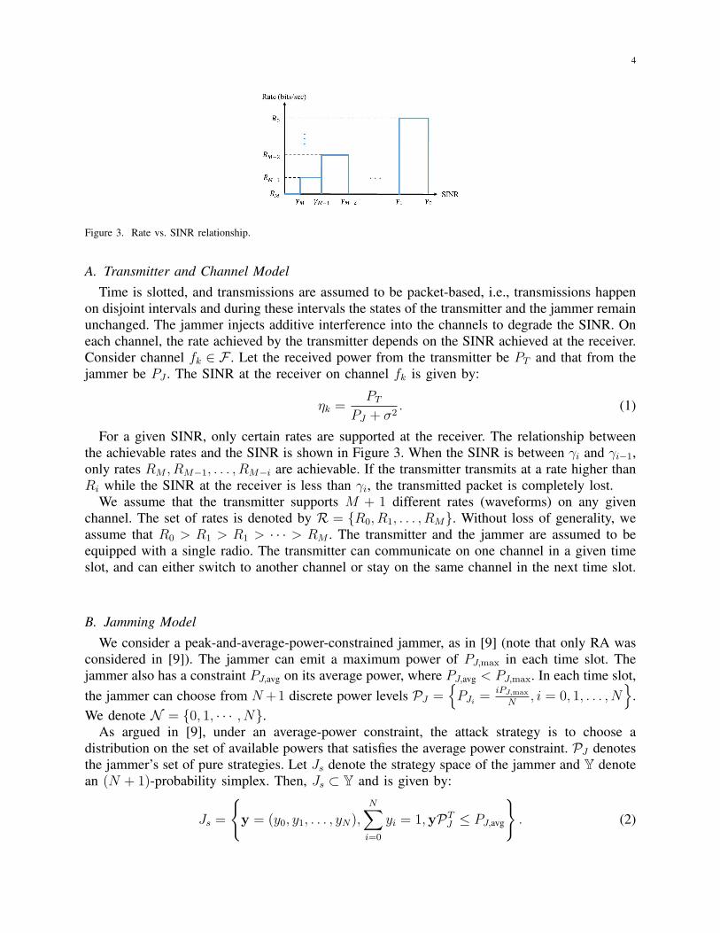
Figure 3. Rate vs. SINR relationship.

A. Transmitter and Channel ModelTime is slotted, and transmissions are assumed to be packet-based, i.e., transmissions happen

on disjoint intervals and during these intervals the states of the transmitter and the jammer remainunchanged. The jammer injects additive interference into the channels to degrade the SINR. Oneach channel, the rate achieved by the transmitter depends on the SINR achieved at the receiver.Consider channel fk ∈ F . Let the received power from the transmitter be PT and that from thejammer be PJ . The SINR at the receiver on channel fk is given by:

ηk =PT

PJ + σ2. (1)

For a given SINR, only certain rates are supported at the receiver. The relationship betweenthe achievable rates and the SINR is shown in Figure 3. When the SINR is between γi and γi−1,only rates RM , RM−1, . . . , RM−i are achievable. If the transmitter transmits at a rate higher thanRi while the SINR at the receiver is less than γi, the transmitted packet is completely lost.

We assume that the transmitter supports M + 1 different rates (waveforms) on any givenchannel. The set of rates is denoted by R = {R0, R1, . . . , RM}. Without loss of generality, weassume that R0 > R1 > R1 > · · · > RM . The transmitter and the jammer are assumed to beequipped with a single radio. The transmitter can communicate on one channel in a given timeslot, and can either switch to another channel or stay on the same channel in the next time slot.

B. Jamming ModelWe consider a peak-and-average-power-constrained jammer, as in [9] (note that only RA was

considered in [9]). The jammer can emit a maximum power of PJ,max in each time slot. Thejammer also has a constraint PJ,avg on its average power, where PJ,avg < PJ,max. In each time slot,the jammer can choose from N+1 discrete power levels PJ =

{PJi =

iPJ,max

N, i = 0, 1, . . . , N

}.

We denote N = {0, 1, · · · , N}.As argued in [9], under an average-power constraint, the attack strategy is to choose a

distribution on the set of available powers that satisfies the average power constraint. PJ denotesthe jammer’s set of pure strategies. Let Js denote the strategy space of the jammer and Y denotean (N + 1)-probability simplex. Then, Js ⊂ Y and is given by:

Js =

{y = (y0, y1, . . . , yN),

N∑i=0

yi = 1,yPTJ ≤ PJ,avg

}. (2)

5

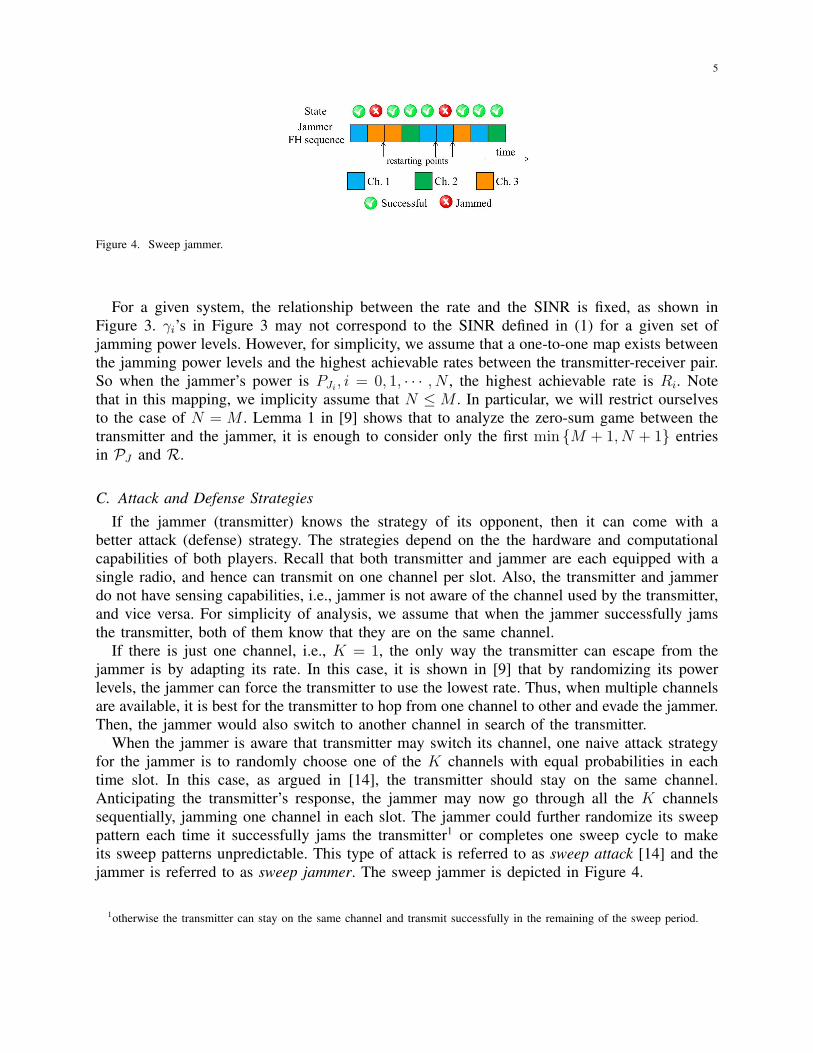
Figure 4. Sweep jammer.

For a given system, the relationship between the rate and the SINR is fixed, as shown inFigure 3. γi’s in Figure 3 may not correspond to the SINR defined in (1) for a given set ofjamming power levels. However, for simplicity, we assume that a one-to-one map exists betweenthe jamming power levels and the highest achievable rates between the transmitter-receiver pair.So when the jammer’s power is PJi , i = 0, 1, · · · , N , the highest achievable rate is Ri. Notethat in this mapping, we implicity assume that N ≤ M . In particular, we will restrict ourselvesto the case of N = M . Lemma 1 in [9] shows that to analyze the zero-sum game between thetransmitter and the jammer, it is enough to consider only the first min {M + 1, N + 1} entriesin PJ and R.

C. Attack and Defense StrategiesIf the jammer (transmitter) knows the strategy of its opponent, then it can come with a

better attack (defense) strategy. The strategies depend on the the hardware and computationalcapabilities of both players. Recall that both transmitter and jammer are each equipped with asingle radio, and hence can transmit on one channel per slot. Also, the transmitter and jammerdo not have sensing capabilities, i.e., jammer is not aware of the channel used by the transmitter,and vice versa. For simplicity of analysis, we assume that when the jammer successfully jamsthe transmitter, both of them know that they are on the same channel.

If there is just one channel, i.e., K = 1, the only way the transmitter can escape from thejammer is by adapting its rate. In this case, it is shown in [9] that by randomizing its powerlevels, the jammer can force the transmitter to use the lowest rate. Thus, when multiple channelsare available, it is best for the transmitter to hop from one channel to other and evade the jammer.Then, the jammer would also switch to another channel in search of the transmitter.

When the jammer is aware that transmitter may switch its channel, one naive attack strategyfor the jammer is to randomly choose one of the K channels with equal probabilities in eachtime slot. In this case, as argued in [14], the transmitter should stay on the same channel.Anticipating the transmitter’s response, the jammer may now go through all the K channelssequentially, jamming one channel in each slot. The jammer could further randomize its sweeppattern each time it successfully jams the transmitter1 or completes one sweep cycle to makeits sweep patterns unpredictable. This type of attack is referred to as sweep attack [14] and thejammer is referred to as sweep jammer. The sweep jammer is depicted in Figure 4.

1otherwise the transmitter can stay on the same channel and transmit successfully in the remaining of the sweep period.

6

III. DFH GAME WITH RATE ADAPTATION

In this section, we develop a repeated-game model between the sweep jammer and thetransmitter, and derive the optimal attack (defense) strategy for the jammer (transmitter). Thedefense strategy is to decide whether to remain on the same channel or switch to another channelin each time slot, and which rate to use. The attack strategy is to choose a jamming power levelin each time slot while satisfying the average-power constraint.

A. Frequency HoppingThe hopping pattern of the sweep jammer is clear– it sweeps all the K channels sequentially,

and if the jammer is successful in destroying a transmitted packet, a new random cycle is restartedimmediately, without completing the previous cycle, see Figure 4. For the transmitter, hoppingis uniform. Each time the transmitter decides to hop, it chooses a channel from the set F withequal probability. We assume that transmitter does not have a means to know the quality of thechannel and assigns no priority to any channel. The transmitter-receiver pair follows a commonFH pattern, generated by a pseudo-random sequence. The receiver hops to the same channel asthe transmitter if it does not hear from the transmitter for a predetermined time.

B. Reward and CostRecall that a transmission at rate Ri is successful if the SINR at the receiver is at least

γi; otherwise, the packet is completely lost. If the transmitter successfully sends at rate Ri, itobtains a reward of Ri units. If the transmission fails, the transmitter incurs a cost of L units.Specifically, a transmission failure disrupts the communication between the transmitter and thereceiver, who need to re-establish their communication through the exchange of several packets,that do not contribute to actual information. Hence, L corresponds to the throughput loss due toa failed transmission. In addition, when the transmitter switches to another channel, it needs towait till the receiver hops onto the same channel. This waiting period can also result in loss inthroughput. We denote the loss in throughput due to channel switching as C units.

In line with [14], we define the transmitter payoff as the difference between the reward andcosts it incurs in each time slot. Let U(n) denote the payoff2 of the transmitter in slot n. Thepayoff is given as:

U(n) =M∑i=0

Ri · 1[successful transmission at rate Ri in slot n]

− L · 1[jamming is successful]−C · 1[transmitter hops],

where 1[A] is the indicator function. We note that only one term can be positive in the summationterm above, as the transmitter can use only one rate in each time slot. An action taken by thetransmitter in a given time slot affects its payoff in future time slots. Thus, we will consider a totaldiscounted payoff with a discount factor δ ∈ (0, 1), which indicates how much the transmittervalues its future payoff over its current payoff. Let U denote the total discounted payoff of thetransmitter. Then, U is given by:

U =∞∑n=0

δnU(n). (3)

2We specify the exact payoff function in the next section after defining state space.

7

We model the interaction between the transmitter and the jammer as a Markov zero-sumgame and derive optimal defense and attack strategies for this game. Note that the jammeris constrained on the average power level. We shall derive constrained Nash equilibria of theMarkov zero-sum game and characterize the properties of the optimal policies using Markovdecision processes.

IV. MARKOV ZERO-SUM GAME

A Markov game is characterized by an action space, immediate reward for each player, and astate space with the transition probabilities. The decision epochs are at the end of time slot, andthe effect takes place in the beginning of the next time slots. The state of the system identifiesthe status of the transmitter. The state is defined as x = (x1, x2), where x1 denotes the numberof contiguous slots since the beginning of the current sweep cycle that the transmitter has beensuccessful and before it last hopped, and x2 denotes the number of time slots the transmitter istransmitting successfully since it last hopped. Each component takes nonnegative integer values.Note that x1+x2 gives the number of time slots the transmitter has been successfully transmittingsince the beginning of the current sweep cycle. The state (0, 0) denotes that the transmitter isjammed (zero successful transmissions). Let X denote the state space. Then, X is given by:

X = {(x1, x2) : x1, x2 = 0, 1, 2, . . . , K}. (4)

At the end of each time slot, the transmitter has to decide whether to stay on the channel itis currently using, or to hop to a randomly selected channel (which may end up being the samechannel). In both cases, the transmitter also has to decide which rate to use from the set R.Therefore, the set of actions available to the transmitter for any state in X is as follows:

A = {(s,R1), . . . , (s,RN), (h,R1), . . . , (h,RN)} (5)

where action (s,Ri) represents the transmitter’s decision to stay in the current channel and userate Ri, and the action (h,Ri) represents the decision to randomly hop to a channel in F and userate Ri on that channel. For notational convenience, we write si = (s, Ri) and hi = (h,Ri). Notethat we allow the transmitter to stay on a channel, irrespective of whether it got jammed or noton that channel in the previous time slot. We write the transmitter’s payoff U(n) as Un(x, a, x

′),which denotes the immediate reward for the transmitter when it enters state x′ in time slot nafter taking action a ∈ A at the end of time slot n − 1 while in state x. We assume that thisreward is the same in each time slot, and drop the subscripts when there is no ambiguity. Forany (a, x) ∈ A×X , the immediate payoff of the transmitter is defined as follows: U(·, a, x)

=

−L− C, ifx = (0, 0), a = hi, ∀i = 1, 2, . . . , N−L, if x = (0, 0), a = si,∀i = 1, 2, . . . , NRi − C, if x = (0, 0), a = hi,∀i = 1, 2, . . . , NRi, if x = (0, 0), a = si,∀i = 1, 2, . . . , N.

(6)

Note that the reward of transmitter depends only on the action it takes and the new state itenters, and not on its current state. Since the jammer cannot observe the state of the transmitter,it just chooses power levels such that its average power is constrained. For any strategy y =(y0, y1, · · · , yN) ∈ Js of the jammer, define Yi =

∑j>i yj for i ∈ N .

We next derive the transition probabilities of the Markov chain (see Figure 5). Let Py(x′|x, a)

denote the transition probability to state x′ when the current state is x and the transmitter chooses

8

Figure 5. Transition probabilities (J denotes jammed state)

action a ∈ A while the jammer uses strategy y. When the current state is (0, 0), the new statecan be either (0, 0) or x = (1, 0), irrespective of what action is taken by the transmitter. Letx = (0, 0). Then, on taking action hi the system enters into state (0, 0) again , only if thejammer also hops onto the same channel as the transmitter and uses a power level that does notallow the transmitter to send at rate Ri. Recall that on each successful jam, the jammer reordershis sweeping pattern independently of his past sweeping pattern. Then, the transmitter and thejammer hop to the same channel with probability 1/K. On the other hand, if the transmitterdecides to stay on the same channel following a successful jamming, the situation will not changeeither, as the jammer randomly reorders the sweeping pattern. Hence, for i ∈ N , we have:

Py((0, 0)/(0, 0), hi) = Yi/K = 1− Py((1, 0)/(0, 0), hi) (7)

Py((0, 0)/(0, 0), si) = Yi/K = 1− Py((1, 0)/(0, 0), si).

When the current state x = (0, 0), say x = (x1, x2), the next state x′ can be either (0, 0),(x1, x2 + 1), or (x1 + x2, 1). Suppose that the transmitter decides to stay on the same channeland use rate Ri. The system then enters into state (0, 0) if jammer hops to the same channel andtransmits at a power that does not allow packet decoding at rate Ri. Note that the jammer canjam the transmitter on a given channel, say f , provided the jammer has not swept through f inthe last x1 + x2 time slots. In this case, it is also clear that the transmitter knows that f has notbeen swept by the jammer in the last x2 slots. However, whether or not the jammer swept thechannel in the first x1 slots is not known to the transmitter. The transition probability for thiscase can be computed as the product of the probability that the jammer has not used channel fin the last x2 slots and the probability that it hops onto f in slot x1 + x2 + 1 given that it hasnot swept f in the past x2 slots. If the transmitter decides to hop and use rate Ri, it will go intostate (x1 + x2, 1) if any of the following happens: (i) the transmitter hops into a channel, sayf , that is already swept by the jammer, (ii) f is not swept by the jammer and the jammer doesnot hop to f in time slot x1 + x2 + 1, or (iii) the jammer hops onto f and uses a power levelthat does not disrupt the transmission at rate Ri. We summarize these transition probabilities asfollows. For i ∈ N , 1 ≤ x1 ≤ K, and 1 ≤ x1 + x2 + 1 ≤ K, we have:

Py((0, 0)/(x1, x2), si) = Yi/(K − x2)

= 1− Py((x1, x2 + 1)/(x1, x2), si). (8)

9

Py((x1 + x2, 1)/(x1, x2), hi) =

1− Py((0, 0)/(x1, x2), hi) =x1 + x2

K

+K − x1 − x2

K

{1− 1

K − x1 − x2

+1− Yi

K − x1 − x2

}= 1− Yi/K. (9)

Remark 1: All transition probabilities depend on the state (x1, x2) only through x2. Henceforth,we denote the state simply as x, which represents the number of successful transmissions ona channel since the transmitter last hopped onto it or since the beginning of the current sweepcycle, whichever occurred later, where x ∈ {0, 1, 2, . . . , K}. With some abuse of notation, weagain use X to denote state space, i.e., X = {0, 1, 2, · · · , K}.

Let ry : X × A → R denote the expected reward for the transmitter when the jammer’sstrategy is y, where R denotes the set of real numbers. For action a in state x, the expectedimmediate reward for the transmitter is given by:

ry(x, a) =∑x′

Py(x′/x, a)U(x, a, x′). (10)

In each time slot, the transmitter takes an action that depends on its past observation. Forsimplicity, we shall restrict ourselves to Markov stationary policies3, where the transmitter takesaction based on his current state only. Let π : X → A denote a decision policy of the transmitter,Πs denote the collection of stationary policies, and π(x) denote the action the transmitter takesin state x ∈ X . For a given π ∈ Πs and a given y, the expected discounted payoff of thetransmitter, when the initial state is x ∈ X is

V (x, π,y) = Eπ,y

{∑n

δnry(Xn, An)| X0 = x

}(11)

where {(Xn, An) : n = 1, 2, . . .} is a sequence of random variables, denoting the state-actionpair in each time slot. This sequence evolves according to the policy pair (π, y). Note that An

consists of the transmitter’s action and the power level chosen by the jammer. The operator Eπ,y

denotes the expectation over the process induced by the policies π and y.The transmitter’s objective is to choose a policy that results in the highest expected reward

starting from any state x ∈ X , defined as

VT (x,y) = maxπ∈Us

V (x, π,y). (12)

In contrast, the jammer’s objective is to choose a strategy y that minimizes the transmitter’sexpected discounted payoff, i.e., ∀x ∈ X ,

VJ(x, π) = miny∈Js

V (x, π,y). (13)

Note that the strategy space of the jammer is constrained, and the transmitter can choose any

3For any given history-dependent policy, there exists a Markov policy that is equally good [15][Ch. 4].

10

stationary policy. We will say a strategy pair (π∗,y∗) is constrained Nash equilibria if y∗ ∈ Jsand

V (x, π,y∗) ≤ V (x, π∗,y∗) ≤ V (x, π∗,y) (14)

for all x ∈ X , π ∈ Πs, and y ∈ Js. Let V ∗(x)def= V (x, π∗,y∗). {V ∗(x), x ∈ N} is referred to as

the values of the zero-sum game4.Theorem 1: The zero-sum game has a stationary constrained Nash equilibria.

Proof: While the jammer aims to minimize the transmitter’s payoff, it needs also to meetits average-power constraint. Since the jammer does not know the value of the current state, itsconstraint on the average power for any strategy y, i.e., yPT ≤ Javg, can be equivalently writtenas a constraint on an expected discounted cost, as follows:

Cβ(π,y) = (1− β)Eπ,y

{∑n≥0

βnC(Xn, An)

}≤ Javg (15)

for some β ∈ (0 1), where C(Xn, An) denotes the cost for the jammer, which is the power itchooses in time slot n. Further, by choosing a strategy y′ such that y′0 = 1, the constraint on theexpected discounted cost is strictly met.

Thus, strong Slater condition in [17] is verified and the existence of stationary constrainedNash equilibria follows from Theorem 2.1 in [17].

A. Optimal Defense Strategy at the TransmitterIn this subsection, we derive the properties of the optimal defense strategy for the transmitter

against a given jammer’s strategy. Let π∗y(X) denote the policy that maximizes the expected

discounted reward function when the jammer uses strategy y. For simplicity, we do not explicitlymention this dependency on y, and write VT (x,y) = V (x) for notational convenience.

We use the value iteration [15][Ch. 6] method to derive the optimal defence strategy and itsproperties. The well-known Bellman equations for the expected discounted utility maximizationproblem in (12) are written as follows:

Q(x, a) = ry(x, a) + δ∑x′∈X

Py(x′|x, a)V (x′)

=∑x′∈X

Py(x′|x, a) {U(x, a, x′) + δV (x′)} (16)

V (x) = maxa∈A

Q(x, a).

Note that in our formulation sates x = 0 and x = K are equivalent, as the jammer will bestarting the sweep cycle afresh at the end of each sweep cycle or after successfully jammingthe transmitter. Hence, when the transmitter begins in either state 0 or state K, it should get thesame total discounted reward, i.e., V (0) = V (K). From (16), for any x = 0, 1, . . . , K− 1, V (x)is expressed in terms of V (0) and V (x + 1). Furthermore, because V (0) = V (K), V cannotbe a monotone function on the set X . However, we enforce the monotonicity by restricting thetransmitters reward in state K − 1, and use this monotonicity property to establish structure ofthe optimal policy.

4If (π, y) is another equilibria, it also results in the same value of the game, i.e., V ∗(x) = V (x, π, y) [16][Sec. 3.1].

11

Figure 6. Optimal policy.

Lemma 1: Let ry(K − 1, a) = 0, for all a ∈ A, i.e., in state K − 1, the transmitter gets zeroreward. Assume RN ≥ δR0. Then, V (·) is a decreasing function over {0, 1, 2 · · · , K − 1}.

From (7) and (9), we note that when the transmitter takes action hi, i ∈ N , the probability ofentering into state 0 or 1 does not depend on the current state. We make use of this observationand the monotonicity of the function V (·) to derive the following structure of the optimal policy.

Proposition 1: The optimal policy π∗ is such that• There exists constants K∗ ∈ {1, 2, · · · , K − 1} and i∗ ≤ N such that

π∗(x) = hi∗ for K∗ ≤ x ≤ K − 1 and π∗(0) = si∗ .

• For any integers x and y, such that 1 ≤ x < y < K∗, and π∗(x) = sj and π(y) = sk, satisfyj ≥ k

• If ry(0, si) is decreasing in index i, then i∗ = 0.Proof: The proof idea is as follows. Note that Q(hi) = Q(x, hi) does not depend on x for

all i ∈ N . We show that Q(x, si) is decreasing in x for all i ∈ N . Then, for for any i ∈ Nthere exists x ∈ X such that Q(x, si) will be smaller than the largest Q(hi). Detailed proof isin the appendix.

The above proposition tells that when a new sweep cycle begins or the transmitter is jammedon a given channel, the transmitter needs to continue to stay on the same channel until itsuccessfully transmits for K∗ consecutive time slots, and hops onto another channel after that.While it stays on a given channel, the transmitter adapts its transmission rate– the transmitterlowers the transmission rate as the number of successive successful transmissions increases.When the transmitter hops, it always uses a fixed rate, which is same as that it uses in the timeslot that follows a successful jamming slot. Further, this rate is the maximum rate available (R0)if ry(0, si) is decreasing in index i.A typical optimal policy is as shown in Figure 6. The x- axis denotes the time index. The stateof the transmitter and the channel used in in each time slot are marked below x-axis. In thispolicy, on completion of a sweep channel or after being jammed, the transmitter stays on thesame channel and uses rate R0. If successful, it uses rate R1 in the next time slot. After itsucceeds to transmit in slot 3 with rate R2 and in time slot 4 with rate R3, it takes the hopdecision and transmits with rate R0. The state changes from 4 to 1 after the hop decision asshown on the x-axis. K∗ = 4 in this policy.

Note that since the transmitter hops once it reaches state K∗, it never enters into the state thatis larger than K∗. Thus, if K∗ < K, the resulting Markov chain is reducible.

Corollary 1: The threshold K∗ is decreasing in L, and increasing in K and C.

12

Proof: The proof follows by noting that for any x′ > x, the difference Q(x′, si)−Q(x, si)is an increasing function in L and a decreasing function in K, for all i ∈ N . Q(x, hi) is adecreasing function in C for all i ∈ N and x ∈ X . This verifies that K∗ is an increasingfunction in C.

Next, we return to the study of the Markov game.

B. Constrained Nash EquilibriaIn this subsection, we give a method to compute constrained-Nash equilibria of the Markov

zero-sum game and study its properties. For a given defense strategy y ∈ Js, the following linearprogram solves the recursive equations in (16) [16][Sec 2.3]:

minimizeV (x)

∑x

V (x)

subject to V (x) ≥ ry(x, a) + δ∑x′∈X

Py(x′|x, a)V (x′)

∀x ∈ X, a ∈ A

(17)

From Theorem 1, we know that the Markov zero-sum game has a constrained Nash equilibria.We use a non-linear version of the above programming method to compute the equilibria. First,we will develop the necessary notation5. Let M(A) denote the distribution on set A and f :X → M(A) denote the strategy of the transmitter. f(x, a) denotes the probability of choosingaction a ∈ A in state x ∈ X . We write f(s) = (f(s, a), a ∈ A). Similarly, denote the jammer’sstrategy as g : X → M(PJ). Since, jammer does not know the state, g(x) = y ∈ Js for allx ∈ X . Let r(s, a, p) denote the immediate reward for the transmitter when transmitter takesaction a ∈ A and the jammer takes action p ∈ PJ in state x, and P (x′|x, a, p) denote thecorresponding transition probability of entering into state x′. Write, R(x) = [r(x, a, p)]a∈A,p∈PJ

and T (x, V ) = [∑

x′ P (x′|x, a, p)]a∈A,p∈PJfor the reward matrix and the transition probability

matrix. R(x) and T (x, V ) matrix are defined as in the previous section– r(x, a, p) for each actionp is obtained similar to ry(x, a) without taking expectation with respect to jammer’s strategy.Consider the following non-linear program:

minimizeV1(x),V2(x)

∑x

V1(x) + V2(x)

subject to V1(x)1 ≥ R(x)gT (s) + δT (x, V1) ∀x ∈ X

V2(x)1 ≥ −f(s)R(x) + δT (x, V2) ∀x ∈ X

PJgT (x) ≤ Javg ∀x ∈ X

(18)

Theorem 2: Let (V ∗1 (x), V

∗2 (x), f

∗(x), g∗(x)) denote the global minimum of the non-linearprogram (18). Then, (f ∗(x), g∗(x)) denotes the optimal constrained Nash-equilibria of the game.

Proof: The nonlinear program (18) is the same as in [16][Sec. 3.7] with the additionalaverage-power constraint on the jammer’s strategy. The proof follows from [16][Th. 3.7.2].

Note that though the optimal strategy of the transmitter for a given strategy of the jammer isdeterministic, the equilibrium strategy may not be deterministic [16][Ch. 2]. The strategy g∗(x) is

5We follow the notational conventions in [16].

13

the same for all x ∈ X as jammer does not know the state. We know from the previous subsectionthat optimal transmitter’s strategy against any given y is deterministic. Thus at equilibrium, thestrategy of the transmitter is deterministic, and can be computed by solving (16) for the strategyy∗ = g∗(s) obtained from (18).

V. MINIMAX Q-LEARNING

In this section we develop a reinforcement algorithm for the transmitter to learn the optimaldefense strategy without explicit knowledge of the jammer. We adapt the Minimax Q-learningalgorithm for the Markov zero-sum games in [18].

If the receiver can listen on all the channels simultaneously, then the receive can quickly learnthe strategy of the jammer by measuring proportion of the times each power level is used bythe jammer and communicate it to the transmitter through a feedback channel. In this case, thetransmitter’s optimal defense strategy is derived in the previous section. However, if the receivercan listen only one channel at a time, then action taken by the jammer (power level) is known6

only when both the transmitter and the jammer are on the same channel.Though the optimal strategy of the transmitter for a given strategy of the jammer is deter-

ministic, the equilibrium strategy may not be deterministic [16][Ch. 2]. Minimax Q-learning isa value-function based reinforcement-learning algorithm specifically designed for the zero-sumgames. The value of the game when there is no constraint on the jammers strategy is given by

Q(x, a, p) = r(s, a, p) + δ∑x′X

P (x′|x, a, p)V (x′)

V (x) = maxπ(x,·)∈M(A)

minp∈PJ

∑a∈A

f(x, a)Q(x, a, p). (19)

The minimax Q-learning algorithms chooses an action in proportion to the reward accumulatedfrom that choice in the past. Specifically, the quality of choosing an action in each state isestimated by replacing (19) with

Qn(Xn, a, p) = (1− µn)Qn−1(Xn, a, p)

+(1− µn)(r(s, a, p) + δV (Xn+1)),

where αn denotes the learning rate.The mininimax Q-algortihm is presented in Algorithm 1. If we set for every state-action pair

µn := µn(x, a, p) =1

(1 + number of updated for Q(x, a, p)),

it converges to the optimal strategy of the transmitter from [19][Th. 4]. Clearly, learning rate forany state-action pair satisfies

∑n µn = ∞ and

∑n µ

2n < ∞.

Proposition 2: The minimax Q-learning update rule converges to the optimal Q-function withprobability 1, provided each state-action pair is infinitely visited.

In step-2, the algorithm deviates from the optimal policy with probability explor and chooses anaction uniformly at random. This step ensures that the state-action space is adequately explored.Linear programming can be used to obtain optimal policy π(s, ·) in Step-4.

6Since the transmitter transmits at a fixed power, receiver can measure the amount of interference in received signal (e.g.,slow fading).

14

Note that the unlike the Q-learning algorithm presented in [14], the minimax Q-learningalgorithm maintains the table for all the possible actions of the jammer. In our case, thetransmitters knows the action of the jammer only when they are on the same channel. When theyare not on the same channel, the transmitter updates the Q(s, a, p)-table assuming that jammerused action P0 in that time slot.

The policy learned by the minimax Q algorithm converges to the optimal policy, and thispolicy is learned in total ignorance of the jammer. Thus, the learned strategy will be optimalagainst any attack by the jammer, and in particular against the sweep attack.

Step-1:Initialization;For all x ∈ X, a ∈ A, p ∈ PJ ;Let Q(x, a, p) = 1, V (x) = 1, π(x, a) = 1/|A|, and α = 1 ;for n = 1, 2, · · · do

Step-2: Choose an action;With probability explor, return a ∈ A uniformly;Otherwise if in state Xn, return a with probability π(s, a) ;step-3:Learn;After receiving reward r for moving from Xn to Xn+1 via action a and opponent’s action p;if a = si, for some i ∈ N then

Qn(Xn, si, p) = (1− α)Qn−1(Xn, si, p) + (1− α)(r + δV (Xn+1));Qn(X, a, p) = Qn−1(X, a, p) for other (X, a, p);

else∀ x ∈ X ,Qn(x, a, p) = (1− α)Qn−1(x, a, p) + (1− α)(r + δV (Xn+1));Qn(X, a, p) = Qn−1(X, a, p) for other (X, a, p)

endStep-4:Update Policy;if |V − V ′| ≤ ϵ stop; elsechoose π(x, ·) for all x ∈ X such that;π(x, ·) = arg max

π′(x,·)min

p′∈PJ

∑a′∈A

π′(x, a′)Qn(x, a′, p′);

V ′(x) = minp′∈PJ

∑a′∈A

π(x, a′)Qn(x, a′, p′);

α = µn, V = V ′

end

Algorithm 1: Minimax Q-learning Algorithm

VI. PERFORMANCE EVALUATION

In this section, we study the performance of the proposed zero-sum Markov game underdifferent values of the system parameters. Our performance metrics are the average goodput (inMbps), the success rate (defined as percentage of un-jammed transmissions), and the hop rate(defined as the rate at which the transmitter switches channel). All performance measures arecomputed over 1000 sweep cycles. The parameters of study include the number of channels K,the jamming cost L, and the switching cost C. For the jammer we set Jmax = 25 and Javg = 20.We followed the rate adaptation system of the IEEE 802.11a protocol [20], which uses rates6, 9, 12, 18, 24, 36, 48, and 54 Mbps. The proposed game is implemented in MATLAB. The95% confidence intervals are shown in the numerical figures. When they are very tight, they are

15

not drawn to prevent cluttering the graph. We obtain the joint-optimal defense strategy of thetransmitter and attack strategy of the jammer by solving (18).

The proposed joint-optimal policy is compared with three other policies: (i) Optimal FH:transmitter switches channels according to the joint-optimal policy, but transmits at fixed rateof 54 Mbps, (ii) Optimal RA: transmitter adapts rate according to the joint-optimal policy, butdoes not switch channels and (iii) Random FH: transmitter hops in each slot, and transmit atfixed rate of 54 Mbps. In the random FH strategy, in each slot the transmitter uniformly selectsone channel, and does not perform any RA.

A. Average GoodputFigure 7 depicts the average goodput vs. L for two values of C. Figure 7(a) shows that when

C is large (in our example, C = 30 Mbps), there is a threshold L∗ on the value of L; if L < L∗

the optimal FH scheme works almost as good as the joint-optimal scheme, and if L > L∗ theperformance of the optimal FH scheme starts degrading with L. This shows the importanceof RA when L is large, given that C is also large. Figure 7(a) also shows that, in contrastto the optimal FH scheme, the optimal RA scheme is worse than the joint-optimal when L issmaller than a certain threshold (not necessarily the same threshold as L∗), and it behaves almostthe same as joint-optimal when L is sufficiently large. The random FH scheme has the worstperformance. This is because of the incurred switching cost due to continuous hopping. WhenC is relatively small (e.g., C = 5 Mbps), Figure 7(b) shows that the optimal FH behaves almostthe same as the joint-optimal, irrespective of the value of L.

The average goodput is plotted in Figure 8 vs. K. When K is sufficiently large (K > 4 inour setup), the optimal FH scheme works almost as good as the joint-optimal scheme, however,if K < 4 the joint-optimal works much better than the optimal FH. In contrast, the optimal RAscheme works close to the joint-optimal scheme when K is small, and its performance degradescompared to the joint-optimal scheme when K is large. As shown in Figure 8, the averagegoodput improves with K.

B. Success RateFigure 9 plots the success rate vs. L for two values of C (C = 30 Mbps and C = 5 Mbps).

When C is small, The success rates of both the optimal FH and the joint-optimal schemes arealmost the same, and they are non-decreasing with L. The success rate of the random FH schemeis ∼ 100%.

When C is large, the success rate of the optimal FH scheme decreases with L, and the achievedimprovement in success rate by jointly optimizing the becomes obvious when L is large (joint-optimal has a success rate of ∼ 89% compared to a success rate of ∼ 67% for the optimalFH when L = 100 Mbps). When L is sufficiently large, success rate of optimal RA is close tosuccess rate to the joint-optimal scheme.

When K = 1, the success rate of both the joint-optimal and the optimal RA scheme is 100%.This is because the transmitter and jammer are both on the same channel and the RA strategywill enforce the transmitter to use the lowest rate (i.e., 6 Mbps. See Figure 7) in order to avoidjamming. The success rate of both schemes drops significantly when K is 2 because in thiscase the jammer starts sweeping between two channels and the transmitter does not know whichchannel is currently used by the jammer. When K > 2, the success rates of both schemes startincreasing with K, but the success rate of the joint-optimal increases faster. For the optimal FH

16

10 20 30 40 50 600

5

10

15

20

25

30

35

Jamming Cost (L) (Mbps)

Ave

rage

Goo

dput

(M

bps)

Joint optimal (DFH and RA)RA OnlyOptimal DFH, Rate = 54 MbpsRandom FH, Rate = 54Mbps

10 20 30 40 50 6015

20

25

30

35

40


Ave

rage

Goo

dput

(M

bps)


(a) C = 30 Mbps (b) C = 5 Mbps

Figure 7. Average goodput vs. L for different values of C (K = 5).

1 2 3 4 5 6 7 8 9 1011121314151617181920−60

−40

−20

0

20

40

60

Number of Channels (K)

Ave

rage

Goo

dput

(M

bps)


Figure 8. Average goodput vs. K (L = 40,C = 22).

strategy, the success rate is zero when K = 1 because the transmitter and jammer are both onthe same channel, and the success rate increases when K increases.

C. Hop RateFigure 11 depicts the hop rate vs. L for two values of C. When C is large, both joint-optimal

and the optimal FH prefer not to hop when L exceeds a certain threshold, and hop with a low rate(< 7%) when L is small enough. When C is small, both schemes prefer hopping frequently, andthe hopping rate increases when L exceeds a certain threshold. Figure 12 plots the hop rate vs.K. Both schemes prefer not to hop for small values of K. When K exceeds a certain threshold,the hop rate of both schemes increase significantly, beyond which the hop rate decreases with Kbecause when K increases the likelihood of meeting the jammer on the same channel decrease,therefore the hop rate decreases.

VII. CONCLUSIONS

In this paper, we analyzed a defense strategy against a sweep jammer that is derived byjointly optimizing frequency hopping and rate adaptation techniques. We modeled the interactionbetween the transmitter and jammer as a Markov zero-sum game and derived optimal equilibriumdefense strategy against the worst attack strategy.

Performance evaluation of the proposed scheme shows that the joint-optimal strategy improvesimproves performance. The joint-optimal scheme is particularly efficient when the number ofchannels is low. When the number of channels is high, optimal FH performs close to joint optimal

17

20 40 60 80 10065

70

75

80

85

90


Succ

ess

Rat

e (%

)

Joint optimal (DFH and RA)RA OnlyOptimal DFH, Rate = 54 Mbps

20 40 60 80 10066

68

70

72

74

76

78

80

82


Succ

ess

Rat

e (%

)



Figure 9. Success rate vs. L for different values of C (K = 5).

1 2 3 4 5 6 7 8 9 10 11 12 13 14 15 16 17 18 19 200

20

40

60

80

100


Succ

ess

Rat

e (%

)


Figure 10. Success rate vs. K (L = 40,C = 22).

10 20 30 40 50 60 70 80 90 1000

1

2

3

4

5

6

7


Hop

Rat

e (%

)

Joint optimal (DFH and RA)Optimal DFH, Rate = 54 Mbps

10 20 30 40 50 60 70 80 90 10020

30

40

50

60

70

80


Hop

Rat

e (%

)



Figure 11. Hop rate vs. L for different values of C (K = 5).

1 2 3 4 5 6 7 8 9 10 11 12 13 14 15 16 17 18 19 200

5

10

15

20


Hop

Rat

e (%

)


Figure 12. Hop rate vs. K (L = 40, C =22).

18

policy. Numerical evaluations show that threshold effect exists on the performance of the optimalFH and optimal RA schemes. For example, when L and C are high, optimal RA performs betterthan optimal FH, but as the value of L decreases optimal FH gives better performance thanoptimal RA. Whereas, the joint optimal scheme gives performance (goodput, success rate, andhop rate) better than both optimal FH and optimal RA for any values of L,C and K. Thus,defense policy derived by jointly optimizing FH and RA techniques achieve better performanceover all the system parameters.

REFERENCES

[1] W. Xu, W. Trappe, Y. Zhang, and T. Wood, “The feasibility of launching and detecting jamming attacks in wirelessnetworks,” in Proc. of the ACM MobiHoc Conf., Urbana-Champaign, IL, USA, 2005.

[2] S. Khattab, D. Mossee, and R. Melhem, “Jamming mitigation in multi-radio wireless networks: Reactive or proactive?” inProc. of the ACM SecureComm Conf., Istanbul, Turkey, September 2008.

[3] R. Gummadi, D. Wetherall, B. Greenstein, and S. Seshan, “Understanding and mitigating the impact of RF interferenceon 802.11 networks,” in Proc. of the ACM SIGCOMM Conf., Kyoto, Japan,, 2007.

[4] E. Bayraktaroglu, C. King, X. Liu, G. Noubir, and R. Rajaraman, “On the performcne of IEEE 802.11 under jamming,”in Proc. of the IEEE INFOCOM Conf., Phoenix, AZ, USA, April 2008.

[5] W. Xu, T. Wood, W. Trappe, and Y. Zhang, “Channel surfing and spatial retreats: defenses against wireless denial ofservice,” in Proc. of the ACM WiSe Workshop, Philadelphia, PA, USA, Ocotber 2004.

[6] V. Navda, A. Bohra, S. Ganguly, and D. Rubenstein, “Using channel hopping to increase 802.11 resilience to jammingattacks,” in Proc. of the IEEE INFOCOM Conf., Anchorage, Alaska, USA, 2007, pp. 2526–2530.

[7] K. Pelechrinis, I. Broustis, S. Krishnamurthy, and C. Gkantsidis, “Ares: An anti-jamming REinforcement System for 802.11networks,” in Proc. of CoNEXT, Rome, Italy, 2009.

[8] J. Zhang, K. Tan, J. Zhao, H. Wu, and Y. Zhang, “A practical SNR-guided rate adaptation,” in Proc. of the IEEE INFOCOMConf., Phoenix, AZ, USA, April 2008.

[9] K. Firouzbakht, G. Noubir, and M. Salehi, “On the capacity of rate-adaptive packetized wireless communication linksunder jamming,” in Proc. of the ACM WiSec Conf., Tucson, AZ, USA, 2012.

[10] K. Pelechrinis, I. Broustis, S. V. Krishnamurthy, and C. Gkantsidi, “A measurement-driven anti-jamming system for 802.11networks,” IEEE/ACM Transactions on Networking, vol. 19, no. 4, pp. 1208–1222, August 2011.

[11] G. Noubir, R. Rajaraman, B. Sheng, and B. Thapa, “On the robustness of IEEE802.11 rate adaptation algorthms againtsmart jamming,” in Proc. of the ACM WiSec conf., Hamburg, Germany, June 2011.

[12] K. Pelechrinis, C. Koufogiannakis, and S. Krishnamurthy, “Gaming the jammer: Is frequency hopping effective?” in Proc.of the ACM WiOpt Conf., Seoul, Korea, June 2009.

[13] H. Gintis, Game Theory Evolving (Second Edition). Princeton University Press, 1990.[14] Y. Wu, B. Wang, K. J. Liu, and T. C. Clancy, “Anti-jamming games in multi-channel cognitive radio networks,” IEEE

Journal on Selected Areas in Communications, vol. 30, no. 1, pp. 4–15, January 2012.[15] M. L. Puterman, Markov Decision Processes: Discrete Stochastic Dynamic Programming. John Wiley & Sons, Inc., 1994.[16] J. Filar and K. Vrieze, Competitive Markov Decision Processes. New York, USA: springer-Verlag, 1997.[17] E. Altman and A. Shwartz, “Constrined Markov games: Nash equilibria,” Advances in Dynamic Games and Applications,

vol. 5, pp. 213–221, 2000.[18] M.L.Littman, “Markov games as a framework for multi-agent reinforcement learning,” in Proc. of the Int’l Conf. on

Machine Learning (ICML), July 1994, pp. 157–163.[19] ——, “Value-function reinforcement learning in Markov games,” Journal of Cognitive Systems Research, vol. 2, pp. 55–66,

2001.[20] “Wireless LAN medium access control (MAC) and physical layer (PHY) specifications,” IEEE Std. 802.11, June 2007.

VIII. APPENDIX

A. Proof of Lemma 1When in state K − 1, the transmitter gets zero reward and enters into state K. From 16 we

have V (K − 1) = δV (K) = δV (0), and for x = 0, 1, 2, · · ·K − 2 and i = 1, 2, · · · , N ,

V (x) ≥ Yi

K − x(−L+ δV (0))

+

(1− Yi

K − x

)(Ri + δV (x+ 1)).

19

First note that by taking i = N , V (x) ≥ RN +δV (x+1). Hence, if we start with positive valuesfor V in the value iteration algorithm the new V is also positive. Implying that V (x) ≥ 0 forx ∈ X . Consider the difference

V (K − 2)− V (K − 1) ≥ Yi

2(−L+ δV (0))

+

(1− Yi

2

)(Ri + δV (k − 1))− V (K − 1).

For i = N , we have

V (K − 2)− V (K − 1)

≥ RN + δV (K − 1)− V (K − 1)

= RN − δ(1− δ)V (0) > 0. (20)

We use the relation V (K − 1) = δV (0) in the last step. The maximum reward the transmittercan get is R0. Then, from (12), we get V (x) ≤ R1

1−δfor x = 0, 1, 2, · · ·K−1. The final positivity

claim follows by using the condition RN ≥ δR0 Following similar steps we can establish themonotonicity in other components.

B. Proof of Proposition 1As the transition probabilities and the reward do not depend on the state when the transmitter

decided to hop, for all i ∈ N and x ∈ X , we have

Q(x, hi) = Q(0, hi) = Q(0, si)− CYi/K ≤ Q(0, si). (21)

It is clear that in state x = 0, ‘stay’ is the optimal strategy. Let Q∗ def= maxi∈N Q(0, hi). Then,

Q∗ < Q(0, si). Note that ry(0, si) = −L(Yi/K)+Ri(1−Yi/K) need not be monotone in indexi, as both Ri and Yi are decreasing in i. By applying (16) for all i ∈ N , we have

V (0) ≥ r(0, si) +Yi

KδV (0) +

(1− Yi

K

)δV (1) (22)

with equality for some i ∈ N . Let m denote this index. Rewriting the above relation withequality for action sm, we have

Ym

K(Rm + L) =

(Rm − (1− δ)V (0)) + δ

(1− Ym

K

)(V (0)− V (1)).

(23)

The left-hand quantity is positive, and the last quantity on the right side is positive by the factthat V (0) ≥ V (1). This implies that it must be the case that Rm ≥ (1 − δ)V (0). We use thisrelation to show that Q(x, sm) is monotonically decreasing in x on the set {0, 1, 2, · · ·K − 1}.

20

Taking the difference of Q(x, sm) and Q(x′, sm) for x ≥ x′, we have

Q(x, sm)−Q(x′, sm) =(1

K − x′ −1

K − x

)Ym(L+Rm − δV (0))

+ δ

(1− Ym

K − x

)V (x+ 1)− δ

(1− Ym

K − x′

)V (x′ + 1)

≥(

1

K − x′ −1

K − x

)Ym(L+Rm − δV (0))

+

(1

K − x′ −1

K − x

)δYmV (x′ + 1) ≥ 0. (24)

We used the relation V (x+ 1) ≥ V (x′ + 1) in the last inequality. Furthermore,

Q(x, sN)−Q(x′, sN) = δ(V (x+ 1)− V (x′ + 1)) > 0. (25)

Using similar arguments we can show that Q(x, si) is decreasing in x for all i ∈ N . Indeed,(24) holds for all i ∈ N when RN ≥ δR0. Since Q(x, si) is decreasing in x and Q∗ < Q(0, si), forall i ∈ N , there exists an integer K∗, 0 < K∗ ≤ K−1, such that Q(K∗−1, si) < Q∗ ≤ Q(K∗, si)for all i ∈ N . In the extreme case where Q(K − 1, si) ≥ Q∗ for all i ∈ N , the transmitteralways stays on the same channel.

The second part of the proposition follows by noting that the difference Q(x, si)−Q(x′, si)for any x > x′ is increasing in index i. To prove the last part of the proposition, first note thatYi is decreasing in index i. Due to the fact that V (0) ≥ V (1), the sum

ry(0, si) +Yi

KV (0) +

(1− Yi

K

)V (1) (26)

is also decreasing in index i. Hence Q∗ = Q(x, h1) and V (0) = Q(0, s1). This completes theproof.

1 game theoretic anti-jamming dynamic frequency hopping

Documents