TREE STRUCTURED NON-LINEAR SIGNAL MODELING

AND PREDICTION

Olivier Michel Alfred Hero Anne Emmanuelle Badel

April 16, 1999

Abstract

In this paper we develop a regression tree approach to identi�cation and predictionof signals which evolve according to an unknown non-linear state space model. In thisapproach a tree is recursively constructed which partitions the p-dimensional state spaceinto a collection of piecewise homogeneous regions utilizing a 2p-ary splitting rule withan entropy-based node impurity criterion. On this partition the joint density of the stateis approximately piecewise constant leading to a non-linear predictor that nearly attainsminimum mean square error. This process decomposition is closely related to a general-ized version of the thresholded AR signal model (ART) which we call piecewise constantAR (PCAR). We illustrate the method for two cases where classical linear prediction isine�ective: a chaotic \double-scroll" signal measured at the output of a Chua-type elec-tronic circuit, and a second order ART model. We show that the prediction errors arecomparable to the nearest neighbor approach to non-linear prediction but with greatlyreduced complexity.

Keywords: non-linear and non-parametric modeling and prediction, regression trees, re-

cursive partitioning, chaotic signal analysis, piecewise constant AR models.

EDICS : SP 2.7, SP 3.9, SP 3.5

Corresponding Author :Olivier MichelLaboratoire de PhysiqueEcole Normale Superieure de LYON46 allee d'Italie69394, LYON cedex 07, FRANCEe-mail:omichel@ens-lyon.frtel: -33 (0) 472 72 83 78fax: -33 (0) 472 72 80 80

1

1 Introduction

Non-linear signal prediction is an interesting and challenging problem especially in appli-

cations where the signal exhibits unstable or chaotic behavior [30, 61, 35]. A variety of

approaches to modeling nonlinear dynamical systems and predicting non-linear signals from

a sequence of N time samples have been proposed [12, 64] including: Hidden Markov Models

(HMM) [24, 25], nearest neighbor prediction [20, 21], spline interpolation [39, 62], radial basis

functions [10], and neural networks [32, 33]. This paper presents a stable low complexity tree-

structured approach to non-linear modeling and prediction of signals arising from non-linear

dynamical systems.

Tree-based regression models were �rst introduced as a non-parametric exploratory data

analysis technique for non-additive statistical models by Sondquist and Morgan [58]. The

regression-tree model represents the data in a hierarchical structure where the leaves of the

tree induce a non-uniform partition of the data space over which a piecewise homogeneous

statistical model can be de�ned. Each leaf can be labeled by a scalar or vector valued non-

linear response variable. Once a cost-complexity metric is speci�ed, known as a deviance

criterion in the book by Breiman etal on classi�cation and regression trees (CART) [9], the

tree can be recursively grown to perform particular tasks such as non-linear regression, non-

linear prediction, and clustering [9, 13, 55, 66]. The tree-based approach has several attractive

features in the context of non-linear signal prediction. Unlike maximum likelihood approaches,

no parametric model is required; however if one is available it can easily be incorporated into

the tree structure as a constraint. Unlike approaches based on moments, since the tree-based

model is based entirely on joint histograms all computed statistics are bounded and stable

even in the case of heavy tailed densities. Unlike most methods, e.g. nearest neighbor,

2

maximum likelihood, kernel density estimation, and spline interpolation, since the tree is

constructed from rank order statistics its performance is invariant to monotonic non-linear

transformations of the predictor variables. Furthermore, as di�erent branches of the tree are

grown independently, the tree can easily be updated as new data becomes available.

Our tree-based prediction algorithm has been implemented in Matlab1 using a k-d tree

growing procedure which is similar but not identical to that of the S-plus function tree()

as described by Clarke and Pregibon [13]. Important features and contributions of this work

are the following:

1. The Takens [19] time delay embedding method is used to construct a discrete time phase

trajectory, i.e. a temporally evolving vector state, for the signal. This trajectory is then

input to the tree growing procedure which attempts to partition the phase space into

piecewise homogeneous regions.

2. The partitioning is accomplished by adding or deleting branches (nodes) of the tree

according to a maximum entropy homogenization principle: we test that the joint prob-

ability density function (j.p.d.f.) is approximately uniform within any node (parent

cell) by comparing the conditional entropy of the data points in the candidate par-

tition of the node (children cells) to the maximum achievable conditional entropy in

that partition. Cross-entropy criteria for node splitting have been used in the past,

e.g. the Kullback-Liebler (KL) \node impurity" measure goes back to Breiman etal [9]

and has been proposed as a splitting criterion for tree-structured vector quantization

(TSVQ) in Perlmutter etal [47]. More recently, Zhang [66] proposed an entropy crite-

rion for multivariate binomial classi�cation trees which is closer in spirit to the method

1The Matlab code is available by request.

3

in this paper. Zhang found that the use of the entropy criterion produces regression

trees that are more structurally stable, i.e. exhibit less variability as a function of N ,

than those produced using the standard squared prediction error criterion. For the

non-linear prediction application, which is the subject of this paper, we have observed

similar advantages using the Pearson Chi-square test of region homogeneity in place of

the maximum entropy criterion of Zhang.

3. Similarly to Clarke and Pregibon [13], a median-based splitting rule is used to create

splits of a parent cell along orthogonal hyperplanes, referred to as a median perpendic-

ular splitting tree in the book by Devroye etal [17]. However, unlike previous methods

which split only along the coordinate exhibiting the most spread, here the median split-

ting rule is applied simultaneously to each of the p coordinates of the phase space vector

producing 2p subcells. This has the advantage of producing denser partitions per node

of the tree and, as the 2p-ary split is balanced only in the case of uniform data, the cell

probabilities in the split can be used directly for homogeneity testing of the parent cell.

4. In order to reduce the complexity of the tree a local singular value decomposition (SVD)

orthogonalization of the phase space data is performed prior to splitting each node. This

procedure, which can be viewed as applying a sequence of local coordinate transforma-

tions, produces a partition of the phase space into polygons whose edges are de�ned

by non-orthogonal hyperplanes. This is similar to the principal component splitting

method proposed for vector quantization of color images by Orchard and Bouman [46],

and other non-orthogonal splitting rules for binary classi�cation trees [17]. However,

for phase space dimension p > 2 our method utilizes all components of the SVD as

contrasted to the principal component alone.

4

5. When applied to non-linear signal prediction in phase space the SVD-based splitting

rule yields a hierarchical signal model, which we call piecewise constant AR (PCAR),

which is a generalization of the non-linear auto-regressive threshold (ART) model, called

SETAR by Tong [61]. This thresholded AR model has been proposed for many physical

signals exhibiting stochastic resonance or bistable/multi-stable trajectories such as ECG

cardiac signals, EEG brain signals, turbulent ow, economic time series, and the output

of chaotic dynamical systems (see references [61] and [31] for examples). A set of

coe�cients of the ART model can be extracted from a matrix obtained as the product

of the local SVD coordinate transformation matrices. A causal and stable model can

then be obtained by Cholesky factorization of this matrix.

6. We give a simple upper bound on the di�erence between the mean squared error of a

�xed regression tree predictor and the minimum attainable mean squared prediction

error. The bound establishes that a �xed regression tree predictor attains the optimal

MSE when the j.p.d.f. is piecewise constant over the generated partition. This bound

can be interpreted as an asymptotic bound on the actual MSE of our regression tree un-

der the assumption that, as the training set increases, the generated partition converges

a.s. to a non-random limiting partition. Many authors have obtained conditions for

asymptotic convergence of tree-based classi�ers and vector quantizers [17, 45, 43, 44].

However, as this theory requires strong conditions on the input data, e.g. independence,

strong mixing, or stationarity, we do not pursue issues of asymptotic convergence in this

paper.

7. It is shown by both simulations and experiments with real data that the non-linear

prediction error performance of our regression tree is comparable to that of the popular

5

but more computationally intensive non-parametric nearest neighbor prediction method

introduced by Farmer [20, 21]. A similar performance/computation advantage of our

regression tree method has been established by Badel etal [10] relative to predictors

based on radial basis functions (RBF).

The outline of the paper is as follows. In Section 2 some background on non-linear

dynamical models and their phase space representation is given. Section 3 continues with

background on regression tree prediction and the basic tree growing algorithm is described.

In Section 4 the local SVD orthogonalization method is described and the equivalence of our

SVD-based predictor to ART is established. Finally, in Section 5 experiments and simulations

are presented.

2 Problem statement

It will be implicitly assumed that all random processes are ergodic so that ensemble averages

associated with the signal can be consistently estimated from time averages over a single

realization.

2.1 Non-linear modeling context

A very general class of non-linear signal models can be obtained by making non-linear modi-

�cations to the celebrated linear ARMA(p,q) model

x(n) =pX

i=1

aix(n� i) +qX

j=0

bje(n� j) (1)

where e(n) is a white Gaussian driving noise with variance �2, and the coe�cients fai; i =

1; : : : ; pg and fbj ; j = 1; : : : ; qg are constants independent of x(n) or en. Let

X(k)n = [x(n� 1) x(n� 2) : : : x(n� k)]T

6

and

E(k0)n = [e(n� 1) e(n� 2) : : : e(n� k0)]T

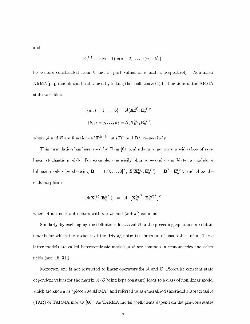
be vectors constructed from k and k0 past values of x and e, respectively. Non-linear

ARMA(p,q) models can be obtained by letting the coe�cients (1) be functions of the ARMA

state variables:

fai; i = 1; : : : ; pg = A(X(k)n ;E(k0)

n )

fbj ; i = j; : : : ; pg = B(X(k)n ;E(k0)

n )

where A and B are functions of IRk+k0 into IRp and IRq, respectively.

This formulation has been used by Tong [61] and others to generate a wide class of non-

linear stochastic models. For example, one easily obtains second order Volterra models or

bilinear models by choosing B = [1; 0; : : : ; 0]T , B(X(k)n ;E(k0)

n ) = BT � E(k0)n , and A as the

endomorphism

A(X(k)n ;E(k0)

n ) = A � [X(k)n

T;E(k0)

n

T]T

where A is a constant matrix with p rows and (k + k0) columns.

Similarly, by exchanging the de�nitions for A and B in the preceding equations we obtain

models for which the variance of the driving noise is a function of past values of x. These

latter models are called heteroscedastic models, and are common in econometrics and other

�elds (see [18, 31]).

Moreover, one is not restricted to linear operators for A and B. Piecewise constant state

dependent values for the matrix A (B being kept constant) leads to a class of non linear model

which are known as \piecewise ARMA" and referred to as generalized threshold autoregressive

(TAR) or TARMA models [60]. As TARMA model coe�cients depend on the previous states

7

X(k)n they belong to the general class of state dependant models developed by Priestley [51].

TARMA models arise in areas of time series analysis including: biology, oceanography, and

hydrology. For more detailed discussion of non-linear models and their range of application

the reader can consult the references [30, 52, 61].

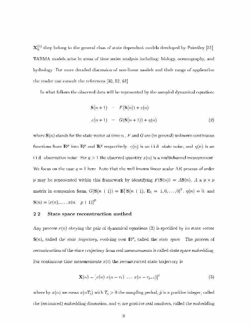
In what follows the observed data will be represented by the sampled dynamical equation:

S(n+ 1) = F (S(n)) + "(n)

x(n+ 1) = G(S(n+ 1)) + �(n) (2)

where S(n) stands for the state vector at time n , F andG are (in general) unknown continuous

functions from IRp into IRp and IRq respectively. "(n) is an i.i.d. state noise, and �(n) is an

i.i.d. observation noise. For q > 1 the observed quantity x(n) is a multichannel measurement.

We focus on the case q = 1 here. Note that the well known linear scalar AR process of order

p may be represented within this framework by identifying F (S(n)) = AS(n), A a p � p

matrix in companion form, G(S(n + 1)) = ET1 S(n + 1), E1 = [1; 0; : : : ; 0]T , �(n) = 0, and

S(n) = [x(n); : : : ; x(n� p+ 1)]T .

2.2 State space reconstruction method

Any process x(n) obeying the pair of dynamical equations (2) is speci�ed by its state vector

S(n), called the state trajectory, evolving over IRp, called the state space. The process of

reconstruction of the state trajectory from real measurements is called state space embedding.

For continuous time measurements x(t) the reconstructed state trajectory is

X(n) = [x(n) x(n� �1) : : : x(n� �p�1)]T (3)

where by x(n) we mean x(nTs) with Ts > 0 the sampling period, p is a positive integer, called

the (estimated) embedding dimension, and �i are positive real numbers, called the embedding

8

delays.

State space reconstruction was �rst proposed by Whitney [65], who stated conditions for

identi�ability of the continuous time state trajectory in the absence of observation noise.

These conditions were formally proved and extended by Takens for the case of non-linear

dynamical systems exhibiting chaotic behavior [19, 59], [11]. In practice only a �nite number

of (generally) equispaced samples are available and the embedding delay is set to �k = k� ,

� = mTs, where m is an integer value. In this �nite case the value used for � is very

important: insu�ciently large values lead to strong correlation or apparent linear dependences

between the coordinates. On the other hand, overly large delays � excessively decorrelate the

components of X(n) so that the dynamical structure is lost [22, 23, 40], and [2, Ch. 3] or [35,

Ch. 9].

Numerous authors have addressed the problem of �nding the best embedding parameters

� and p (see e.g. [22, 23, 40] for detailed discussion). Selection of the dimension p requires

investigation of the e�ective dimension of the space spanned by the estimated residuals. Over-

estimation of p creates state reconstructions with excessive variance while underestimation

creates overly smooth (biased) reconstructions. A widely used method (see [2] or [35] for a

discussion on this topic) which we will use for estimating p is the following: if p > p, the true

state dimension, then the estimated trajectories will lie on a lower dimensional manifold in IRp.

This occurrence can be detected by testing a trajectory-dependent dimensionality criterion,

e.g. the behavior of the algebraic dimension of the state trajectory vectors as p is increased

[38]. We will adopt here the method of Fraser [22] for selection of � : � equals the time at

which the �rst zero of the autocorrelation function occurs, i.e � = minf� > 0 : C(�) = 0g

9

where

C(�) =1

N � 1

Xk

x(k)x(k + �):

3 Growing the Tree

In this section we discuss the construction of the tree-structured predictor and give a bound

on the mean squared prediction error of any �xed tree for the case that p = p. As above

let X(n) = [x(n � 1); : : : ; x(n � p)]T be a state vector of dimension p. A p-th order tree-

structured predictor implements a regression function bx(n) = g(X(n)) which is piecewise

constant as X(n) ranges over cells �k in a partition f�kg of IRp [13]. The most common tree

growing procedure [66, 9, 13] for regression and classi�cation tries to �nd the partition of the

phase space such that the predictive density f(x(n)jx(n� 1); : : : ; x(n� p)) is approximately

constant as the predictor variables x(n � 1); : : : ; x(n � p) vary over any of the partition

cells. As is shown below, if the tree growing procedure does this sucessfully, the tree-based

predictor bxp(n) can attain mean squared error which is virtually identical to that of the

optimal predictor E[x(n)jx(n� 1); : : : ; x(n� p)].

3.1 Regression Tree as a Quantized Predictor

Let I�k(X(n)) be the indicator of the partition cell �k and de�ne the vector quantizer function

Q(X(n)) =LX

k=1

qkI�k(X(n));

where qk = [qk1; : : : ; qkp]T is an arbitrary point in �k. Typically, qk is taken as the centroid of

region �k but this is immaterial in the following. Since the predictor function bx(n) = g(X(n))

is piecewise constant it is obvious that g(X(n)) = g(Q(X(n))), i.e. the tree-structured pre-

dictor can be implemented using only the quantized predictor variables Q(X(n)). Therefore,

given the partition f�kg, the optimal tree-based predictor can be constructed from the multi-

10

dimensional histogram (the partition cell probabilities) as the conditional mean of x(n) given

the vector Q(X(n)).

3.2 A Bound on MSE of Tree-structured Predictor

It follows from Theorem 1 in the Appendix that if the conditional density f(x(n)jX(n)) is

(Lipschitz) continuous of order � within all partition cells of the partition f�kg of IRp, the

mean squared error Eh(x(n)�E[x(n)jQ(X(n))])2

iof the tree-structured predictor satis�es

the following bound:

0 � Eh(x(n)�E[x(n)jQ(X(n))])2

i�E

h(x(n)�E[x(n)jX])2

i� 2max

iK�im

2xE[kX �Qo(X)k�]; (4)

where Qo(X(n)) is the minimum mean squared error quantizer on f�kg, mx is an upper

bound on the mean squared valued of x(n) given X(n), and K�k is a Lipschitz constant

characterizing the modulus of continuity within �k. The upper bound in (4) is decreasing in

the minimum �-th power quantization error E[kX(n)�Qo(X(n))k�] associated with optimal

vector quantization of the predictor variables. Bounds and asymptotic expressions exist for

this quantity [29, 42] which can be used to render the upper bound (21) more explicit, however

this will not be explored here.

Note that the upper bound in (4) is decreasing in maxiK�i and equals zero when f(x(n)jX(n))

is piecewise constant in X(n), i.e. f(x(n)jX(n) = x) =P

i f(x(n)jqi)I�i(x) where qi 2 �i are

arbitrary. Thus in the case of a piecewise uniform conditional density, the optimal predictor

of x(n) given quantized data Q(X(n)) is identical to the optimal non-linear predictor given

unquantized data X(n), i.e. the tree-structured predictor attains the minimum possible pre-

diction MSE. Note that for a general conditional density, both E[kX�Qo(X)k�] and the total

variations fK�kg decrease as the sizes of the partition cells f�kgi decrease. Hence the mean

square prediction error can be seen from (4) to improve monotonically as the conditional

11

density f(x(n)jX(n)) becomes well approximated by the staircase function f(x(n)jQ(X(n))

over X(n) 2 IRp. This forms the basis for tree-based non-linear prediction as explained in

more detail below.

3.3 Branch Splitting and Stopping Rules

Here we describe the generic recursive procedure used for growing the tree from training data.

Let p be an estimate of the phase space dimension p of the signal. Assume that at iteration l

of the tree growing procedure we have created a partition �l and consider the partition cells

�li, which we call the i-th parent nodes at depth l. We re�ne the partition �l by recursively

splitting each partition cell �li into 2p smaller cells which are called children-nodes of the i-th

parent.

To control the number of nodes of the tree we test the residuals in each partition element

of �l against a uniform distribution. If the test for uniformity fails in a particular cell, that

cell is split and 2p parent nodes at depth l + 1 are created. Otherwise the cell is not split

and is declared a terminal node. The set of terminal nodes are called the leaves of the tree.

See Fig. 1 for a graphical illustration of the generic tree growing procedure. The �nal tree

speci�es a set of leaves �1; : : : ; �L partitioning the state-space together with the empirical

histogram (cell occupancy rate): bpj = P (X 2 �j) = N�j=N , where N�j is the number of

samples fX(k)gNk=1 which fall into leaf �j.

3.3.1 Cell Uniformity Test

Here we discuss the selection of the goodness-of-split criterion that is used to test uniformity.

As above letX(k) denote the p-dimensional vector sampled at time kTs, where the reconstruc-

tion dimension p is �xed. Many discriminants are available for testing uniformity including

Kolmogorov-Smirnov tests [37], rank-order statistical tests [16], and scatter matrix tests [26].

12

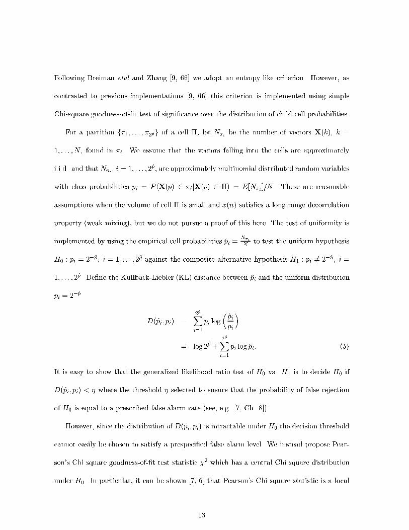
Following Breiman etal and Zhang [9, 66] we adopt an entropy-like criterion. However, as

contrasted to previous implementations [9, 66] this criterion is implemented using simple

Chi-square goodness-of-�t test of signi�cance over the distribution of child cell probabilities.

For a partition f�1; : : : ; �2pg of a cell �, let N�i be the number of vectors X(k), k =

1; : : : ; N , found in �i. We assume that the vectors falling into the cells are approximately

i.i.d. and that N�i , i = 1; : : : ; 2p, are approximately multinomial distributed random variables

with class probabilities pi = P (X(p) 2 �ijX(p) 2 �) = E[N�i ]=N . These are reasonable

assumptions when the volume of cell � is small and x(n) satis�es a long range decorrelation

property (weak mixing), but we do not pursue a proof of this here. The test of uniformity is

implemented by using the empirical cell probabilities pi =N�i

N to test the uniform hypothesis

H0 : pi = 2�p; i = 1; : : : ; 2p against the composite alternative hypothesis H1 : pi 6= 2�p; i =

1; : : : ; 2p. De�ne the Kullback-Liebler (KL) distance between pi and the uniform distribution

pi = 2�p

D(pi; pi) =2pXi=1

pi log

�pipi

�

= log 2p +2pXi=1

pi log pi: (5)

It is easy to show that the generalized likelihood ratio test of H0 vs. H1 is to decide H0 if

D(pi; pi) < � where the threshold � selected to ensure that the probability of false rejection

of H0 is equal to a prescribed false alarm rate (see, e.g. [7, Ch. 8]).

However, since the distribution of D(pi; pi) is intractable under H0 the decision threshold

cannot easily be chosen to satisfy a prespeci�ed false alarm level. We instead propose Pear-

son's Chi square goodness-of-�t test statistic �2 which has a central Chi square distribution

under H0. In particular, it can be shown [7, 6] that Pearson's Chi square statistic is a local

13

approximation to the KL distance statistic (5) in the sense that

D(pi; pi) =1

2N��2 + o(max

i(pi � pi)

2);

where �2 = N�P2p

i=1(pi�pi)2

piis distributed as a central Chi square with 2p � 1 degrees of

freedom undr H0.

3.3.2 Separable Splitting Rule

Another component of the procedure for growing a tree is the method of splitting parent cells

into children cells. The standard cell splitting rule attempts to create a pair of rectangular

subcells for which all marginal probabilities are identical regardless of the underlying distri-

bution. The median-based binary splitting method for constructing k-d trees [5, 15, 13, 17] is

commonly used for this purpose. As the median is a rank order statistic this gives the prop-

erty that the predictor is invariant to monotone transformations of the predictor variables,

a property not shared by most other non-linear predictors. Here we present a variant of the

standard median splitting rule which generates 2p rectangular children cells which only have

equal probabilities when the data is uniform over the parent cell. A version of this 2p-ary

splitting rule which generates non-rectangular cells is discussed in Section 4.

Let �pi=1[�i; �i] denote the hyper-rectangle constructed from the Cartesian product of

intervals [�i; �i], �i < �i, e.g. �2i=1[�i; �i] = [�1; �1] � [�2; �2] is a right parallelepiped

in IR2. We start with a partition element � = �pi=1[�i; �i]. Let this partition element

contain N� of the reconstructed state vectors fX(k)gNk=1. De�ne the N�-element vector

Xj� = [eTj X(k) : X(k) 2 �; k = 1; : : : ; N ] as the projection of the inscribed reconstruction

vectors onto the j-th coordinate axis. That is Xj� is the set of j-th coordinates of those X(k)

falling into �, k = 1; : : : ; N . Denote by bT j� the sample median of the j-th coordinate axis

14

projections

bT j� = medianfeTj X(k) : X(k) 2 �; k = 1; : : : ; Ng:

where, for a scalar sequence fxigni=1, the sample median is a threshold such that half fall to

the left and half to the right:

medianfxig =(

x(n=2); n even

x([n+1]=2); n odd

and x(1) � : : : � x(n) denotes the rank ordered sequence. Note that when the points fX(k)gk

are truly uniform over parent cell the medians f bT j�gj will tend to be near the midpoints of

the edges of the parent cell.

The standard median tree implements a binary split of parent cell � about a hyperplane

perpendicular to that coordinate axis j having the largest spread of points Xj� where the

hyperplane intersects this coordinate axis at the median bT j�. This produces a pair of children

cells which contain an identical number of points. In contrast, we split � into 2p rectangular

children cells whose edges are de�ned by all p perpendicular hyperplanes of the form: fX :

eTj X = bT j�g, j = 1; : : : ; p. This produces a tree with a denser partition than the standard

median tree having the same number of nodes. Unlike the standard median splitting rule

tree, these 2p children cells will not have identical numbers of points unless the points are

truly uniform over �. This allows the cell occupancies in the 2p-ary split to be used directly

for uniformity testing as described in the previous section.

3.3.3 Stopping Rule

The last component of the tree growing procedure is a stopping rule to avoid over-�tting. As

above, de�ne Xj� = feTj X(k) : X(k) 2 �; k = 1; : : : ; Ng as the j-th coordinates of the vectors

X(k) falling into the hyper-rectangle � =�pi=1[�i; �i]. Thus each of the elements of Xj

� lies

in the interval [�j ; �j ]. Under the assumption that these elements are i.i.d. with continuous

15

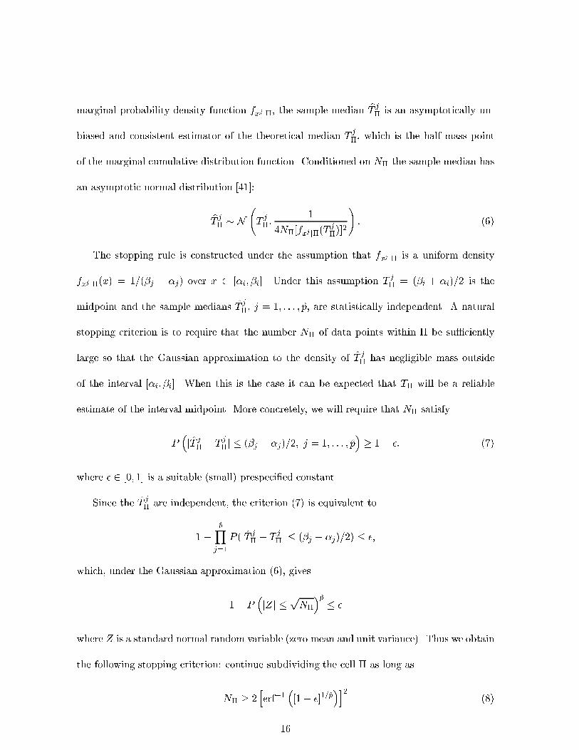
marginal probability density function fxj j�, the sample median bT j� is an asymptotically un-

biased and consistent estimator of the theoretical median T j�, which is the half mass point

of the marginal cumulative distribution function. Conditioned on N� the sample median has

an asymptotic normal distribution [41]:

bT j� � N

T j�;

1

4N�[fxj j�(Tj�)]

2

!: (6)

The stopping rule is constructed under the assumption that fxj j� is a uniform density

fxj j�(x) = 1=(�j � �j) over x 2 [�i; �i]. Under this assumption T j� = (�i + �i)=2 is the

midpoint and the sample medians T j�, j = 1; : : : ; p, are statistically independent. A natural

stopping criterion is to require that the number N� of data points within � be su�ciently

large so that the Gaussian approximation to the density of T j� has negligible mass outside

of the interval [�i; �i]. When this is the case it can be expected that T� will be a reliable

estimate of the interval midpoint. More concretely, we will require that N� satisfy

P�jT j

� � T j�j � (�j � �j)=2; j = 1; : : : ; p

�� 1� �: (7)

where � 2 [0; 1] is a suitable (small) prespeci�ed constant.

Since the T j� are independent, the criterion (7) is equivalent to

1�pY

j=1

P (jT j� � T j

�j � (�j � �j)=2) � �;

which, under the Gaussian approximation (6), gives

1� P�jZj �

pN�

�p � �

where Z is a standard normal random variable (zero mean and unit variance). Thus we obtain

the following stopping criterion: continue subdividing the cell � as long as

N� � 2herf�1

�[1� �]1=p

�i2(8)

16

where erf(x) = 2p�

R x0 e�t

2dt. Use of the asymptotic representation 1 � erf(x) = erfc(x) =

e�x2=(xp�) + o(1=x) [3, 26.2.12] gives the log-linear small � version of (8)

N� � 2 ln

�2p

�

�: (9)

The right hand side of the inequality (8) is plotted as a function of � for several values of

p in Fig. 2. Note that as predicted by the asymptotic (small �) bound (9) the curves are

very close to log linear in �. As a concrete example, the criterion � = 0:01 (99 percent of

Gaussian probability mass is inside �) gives for p = 2: N� = 8, and for p = 4: N� = 10, as

the minimum number of data points N� for which a cell will be further subdivided. These

numbers are of the same order as those obtained from the volume estimation criterion used

by Badel etal [6].

3.4 Computational cost

The steps outlined in the preceding subsections may be summarized by the following tree

growing algorithm:

17

1. input sampled time series and embedding parameters, (p; �), Pearson's �2 test threshold

2. initialize �0 = set of all state vectors

3. while non-empty non-terminal leaves exist, at current depth l

4. for each cell �l

5. if �l contains N�l � p24p�1 vectors

6. compute the splitting thresholds T j�l ; j = 1; : : : ; p

7. estimate empirical probabilities at depth l + 1 for the children of �l

8. Compute Pearson's �2 statistic from the 2p probabilites

9. if �2 is less than threshold

10. �l is stored as a terminal leaf

11. else

12. fT j�l ; j = 1; : : : ; pg are stored

13. f�l+1k ; k = 1; : : : ; 2pg are stored

14. endif

15. else �l is stored as an 'empty' terminal leaf

16. endif

17. endfor

18. l=l+1;

19. goto line 3.

The computational cost associated with this tree estimation algorithm is signal dependent.

For example, in the case of a state space containing N realizations of a p-dimensional white

noise, the trivial partition �0 = IRp will generally pass the uniformity test and the algorithm

will stop at the root node. In this case, only a very few computations are needed. In the

following, we give an estimate of the worst case cost occurring when the terminal nodes all

occur at the same depth.

At depth l of the tree, under the assumption that all obtained cells were stored as non-

empty, non-terminal leaves, the tree has 2pl cells. The average number of p-dimensional

vectors in each leaf is

< N�l >=N�0

2pl:

The most computation consuming step in the algorithm is the splitting threshold determi-

nation procedure which requires rank ordering each of the coordinates of the inscribed state

18

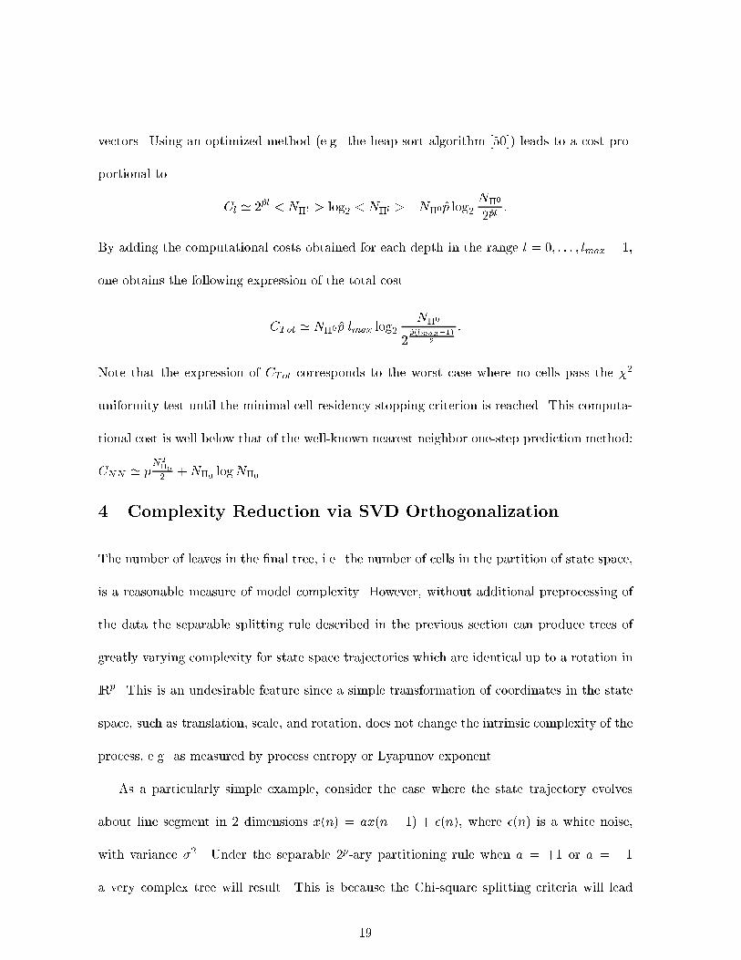
vectors. Using an optimized method (e.g. the heap-sort algorithm [50]) leads to a cost pro-

portional to

Cl ' 2pl < N�l > log2 < N�l >= N�0 p log2N�0

2pl:

By adding the computational costs obtained for each depth in the range l = 0; : : : ; lmax � 1,

one obtains the following expression of the total cost

CTot ' N�0 p lmax log2N�0

2p(lmax�1)

2

:

Note that the expression of CTot corresponds to the worst case where no cells pass the �2

uniformity test until the minimal cell residency stopping criterion is reached. This computa-

tional cost is well below that of the well-known nearest neighbor one-step prediction method:

CNN ' pN2�02 +N�0 logN�0 .

4 Complexity Reduction via SVD Orthogonalization

The number of leaves in the �nal tree, i.e. the number of cells in the partition of state space,

is a reasonable measure of model complexity. However, without additional preprocessing of

the data the separable splitting rule described in the previous section can produce trees of

greatly varying complexity for state space trajectories which are identical up to a rotation in

IRp. This is an undesirable feature since a simple transformation of coordinates in the state

space, such as translation, scale, and rotation, does not change the intrinsic complexity of the

process, e.g. as measured by process entropy or Lyapunov exponent.

As a particularly simple example, consider the case where the state trajectory evolves

about line segment in 2 dimensions x(n) = ax(n � 1) + �(n), where �(n) is a white noise,

with variance �2. Under the separable 2p-ary partitioning rule when a = +1 or a = �1

a very complex tree will result. This is because the Chi-square splitting criteria will lead

19

to a tree with cell sizes on the order of magnitude of �. This is troublesome, as a simple

rotation of the axis coordinates by an angle of �=4 will lead the partitioning algorithm to

stop at the root node. Here we perform a local recursive orthogonalization of the state

vector prior to node splitting in order to produce trees with fewer leaves. This produces

a new orthogonalized sequence of node variables Z�ljwhich are used in place of X�lj

to

perform separable splitting and goodness-of-split tests discussed in the previous section. The

local recursive orthogonalization described below di�ers from a similar principal component

orthogonalization for binary partitioning, �rst described by Orchard and Bouman [46], in that

all the components of the SVD are utilized for the 2p-ary partition used in this paper.

4.1 Local Recursive Orthogonalization

We recursively de�ne a set of orthogonalized node variables as follows. Let X be a p �

N matrix of samples X(k), k = 1; : : : ; N , of the p-dimensional state trajectory. Let the

covariance of X(k) be denoted �X and let it have the SVD (eigendecomposition) �X =

MTXdiag(�X(k))MX. De�ne the root node �0 = IRp. Next de�ne the orthogonalized set of

vectors Z�0

Z�0 =MX(X�E[X]):

The matrix Z�0 is now used in place of X to determine the split of the root node into children

�11 ; : : : ; �12p

according to the same separable splitting and stopping criteria as before. In

practice the empirical mean X = 1NX1 and empirical covariance (X� X)(X� X)T =(N � 1)

are used in place of E[X] and �X.

Now assume a split occurs at the root node and de�ne Z0�1jas the matrix of columns of Z�0

which lie inside �1j . The (empirical) mean and covariance matrix �Z0

�1j

of Z0�1jare computed.

Next the unitary matrix MZ0

�1j

of eigenvectors of �Z0

�1j

is extracted via SVD. This unitary

20

matrix is applied to Z0�1j

to produce an equivalent but uncorrelated set of vectors Z�1j:

Z�1j=M

Z0

�1j

(Z0�1j�E[Z0

�1j]) +E[Z0

�1j]1T�1

j

where 1T�1j

stands for the transpose of the vector containing N�1jones. Application of this

local orthogonalization procedure over all 2p hyper-rectangles �11; : : : ; �12p

produces a set of

local coordinate rotations which results in changing the shape of the hyper-rectangles into

hyper-parallelepipeds. When this process is repeated these hyper-parallelepipeds are further

subdivided producing, at termination of the algorithm, a partition of the state space into

general polytopes �1j .

The general recursion from depth l to depth l + 1 can be written as

Z�l+1j= M

Zl

�l+1j

Zl�l+1j

+Cl1T�l+1j

(10)

where Cl = E[Zl�l+1j

]�MZl

�l+1j

E[Zl�l+1j

].

4.2 Relation to Piecewise Constant AR (PCAR) models

Once the tree growing procedure terminates the partitions �lj can be mapped back to the

original state space by a sequence of backward recursions which back-projects the �l+1j node

variables Z�l+1j

into the parent cell �l via the relation

Zl�l+1j

= MT

Zl

�l+1j

(Z�l+1j�C�l); (11)

Iteration of (11) over l yields an equation for back-projection of Z�l+1jto the root node. By

induction on l the forward recursion (10) gives the relation

Z�l = M�lX�l � C�l1T�l (12)

where X�l denotes the subset of columns of X that are mapped to terminal node �l at depth l

via the sequence of bijective maps (10),M�l and C�l are matrices formed from the telescoping

21

series

M�l =lY

i=0

MZi

�l(13)

C�l =lX

i=0

24 lYj=i

MZj

�l

35C�i (14)

where MZ0

�lis de�ned as the p-dimensional identity matrix.

For any parent node �l the covariance matrix of the rotated data Z�l is diagonal, which

means that the components of Z�l are separable (in the mean squared sense) but not nec-

essarily uniform. On this rotated data the Chi-square test for uniformity can easily be im-

plemented on a coordinate-by-coordinate basis. When the tree growing procedure terminates

we will have found a set of partition cells �l11 ; : : : ; �lLL such that each �l = �lj contains points

Z�l which are (approximately) uniformly distributed over �l. Thus, relation (12) gives an

autoregressive AR(p-1) model whose coe�cients are piecewise constant over regions of state

space X�l .

This can be made more transparent by writing the i-th component of relation (12) as

x(n) = �p�1Xj=1

a�l(i; j)x(n � j) + w�l(n); X(n) 2 �l (15)

where a�l(i; j) = m�l(i; j + 1)=m�l(i; 1), m�l(i; j) denotes the i; j element of M�l , and

w�l(n) = (Z�l(n) + C�l1T�l)ei1 is a white noise.

Note that the coe�cients for the PCAR representation (15) may not be stable. There

is an alternative approach to orthogonalizing the node variables which uses Gramm-Schmidt

recursions and guarantees that all PCAR coe�cients are stable. This method is equivalent

to constructing the Schur complement by adding one coordinate to each vector in the node;

amounting to recursively synthesizing a local stable AR(p-1) model over p = 1; 2; 3; : : :. This

is tantamount to performing Cholesky (LDU) factorization of the local covariance matrices

22

�Zl

�1+1j

[56] as contrasted with the SVD factorization described above. In the sequel the

former method will lead to what will be called a Schur-Tree while the latter will lead to a

tree called the SVD-Tree.

The PCAR model (12) is a generalization of the AR-threshold (ART) model, called SE-

TAR in Tong [61]. Similarly to the PCAR model (12), SETAR is an AR model whose

coe�cients are piecewise constant over regions of state space; but unlike the PCAR model

these regions are restricted to half planes. In particular a 2-level single coordinate p-th order

SETAR model is

x(n) =

(a10 + a11x(n� 1) + : : :+ a1dx(n� p) + �1�(n) if x(n� d) � T0a20 + a21x(n� 1) + : : :+ a2dx(n� p) + �2�(n) if x(n� d) > T0

(16)

where d 2 f1; : : : ; pg. As far as we know, �ltering, prediction, and identi�cation of SETAR

models have only been studied for the case where the switching of the AR coe�cients de-

pends on a single coordinate x(n � d) and where the switching threshold T0 is known. The

PCAR generalization of SETAR models allows transition thresholds to be applied to linear

combinations of past values. As will be illustrated below, the orthogonalized version of the

tree based partitioning algorithm is well adapted to �ltering, prediction and identi�cation

over these models.

5 Examples and Applications

In this section the tree-structured predictors are applied to various real and simulated data

examples.

5.1 Illustrative Examples

To illustrate the parsimony of the local recursive orthogonalization method, we �rst consider

a rather arti�cial random process which follows a piecewise linear trajectory through state

23

space (see Figure (3)). A trajectory made of three linear segments in a 2 dimensional state

space was simulated. The segments have slopes 1.25, -.25 and -2.5 respectively.

Each segment contains 128 realization of the 2 dimensional state vector. White Gaussian

i.i.d. noise of variance �2 = 5 was added to the trajectory. We �rst applied the recursive tree

(RT) method in p = 2 state dimensions without SVD orthogonalization. Both the rectangular

partition of the state space (a) and the tree partitioning algorithm (b) exhibit high complexity.

The number of terminal leaves of the resulting quad-tree is driven exclusively by the variance of

the additive noise. We next grew a quad-tree using the local recursive SVD orthogonalization

procedure, which will be called SVD-Tree here, described in Section 4. The orthogonalization

procedure re-expresses the state vectors in their local eigenbases at each splitting iteration

and, as seen from Figure 4, produces a tree partitioning of lower complexity with many fewer

leaves. As explained in Section 4, applying the recursive SVD orthogonalization on a cell �lj

synthesizes the local AR(1) model (recall (15)

x(n) = �a�ljx(n� 1) + w�l

j(n); [x(n); x(n� 1)] 2 �lj :

We denote by Alj = [1; a�lj

]=r1 + a2

�lj

the unit-length vector of the AR model synthesized in

the cell �lj . Figure 4-c plots the set of unit-length vectors for all cells �lj resulting from the

SVD-Tree partition.

The length of each segment is plotted proportionally to the number of points falling into

the corresponding cell. Note that this graphical representation clearly reveals the existence

of 3 distinct linear segments governing the state trajectories.

5.2 Chua Circuit Experiments

We ran experiments on a physical chaotic voltage waveform, measured at the output of a

\double-scroll' Chua electronic circuit (see [40], [63], [49]).

24

The non-linear di�erential equations governing the Chua circuit are :8><>:dxdt = �(y � )dydt = x� y + zdzdt = ��y

(17)

We built the circuit from \o� the shelf" components chosen so as to get the following set of

parameter values � = 9, � = 1007 , m0 = �1

7 and m1 =27 . The voltage signal at the output

of the electronic circuit was digitized. The sampling frequency was 14.4 kHz. We chose an

embedding dimension p = 4 to generate the state trajectory X(k) = [x(k); x(k � �); x(x �

2�); x(k � 3�)]T . We used a stopping threshold of N� > 16 data points which corresponds

to � ' 3:10�3 (for p = 4) via relation (8). The reconstruction delay � was chosen in such

a way as to minimize the mutual information between the coordinates (see [23] and [19]):

in this case, � = 4 sampling periods. A training set of N�0 = 8192 points was used to

grow the Schur-Tree and obtain the empirical histogram fNi=Ng on the leaves f�ig of the

tree. A non-linear predictor of x(n) given x(n � 1); : : : ; x(n � p + 1) was implemented by

approximating the conditional mean x(n) = E[x(n)jx(n � 1); : : : ; x(n � p + 1)] using the

tree-induced vector quantizer function Q() and the empirical histogram. Speci�cally, with

Q(x(n); : : : ; x(n� p+ 1)) =P

i qiI�i(x(n); : : : ; x(n� p+ 1))

bx(n) =

Ppj=1 �j1

bP (�j1; qn�1; : : : ; qn�p+1)Ppj=1

bP (�j1; qn�1; : : : ; qn�p+1); (18)

where f�ig are centroids of the partition cells f�ig at the leaves of the tree, �j1 denotes the 1-st

element of the vector �j, qn�1; : : : ; qn�p+1 are the 2-nd through p-th elements of the vector

Q(x(n); : : : ; x(n� p+ 1)), and P (q) = 1N

PiNiI�i(q) is the empirical histogram indexed by

q.

Figures 5.a and 5.b show time segments of actual measured and predicted output Chua

circuit voltages using the Schur-Tree predictor and the popular but costlier nearest neighbor

25

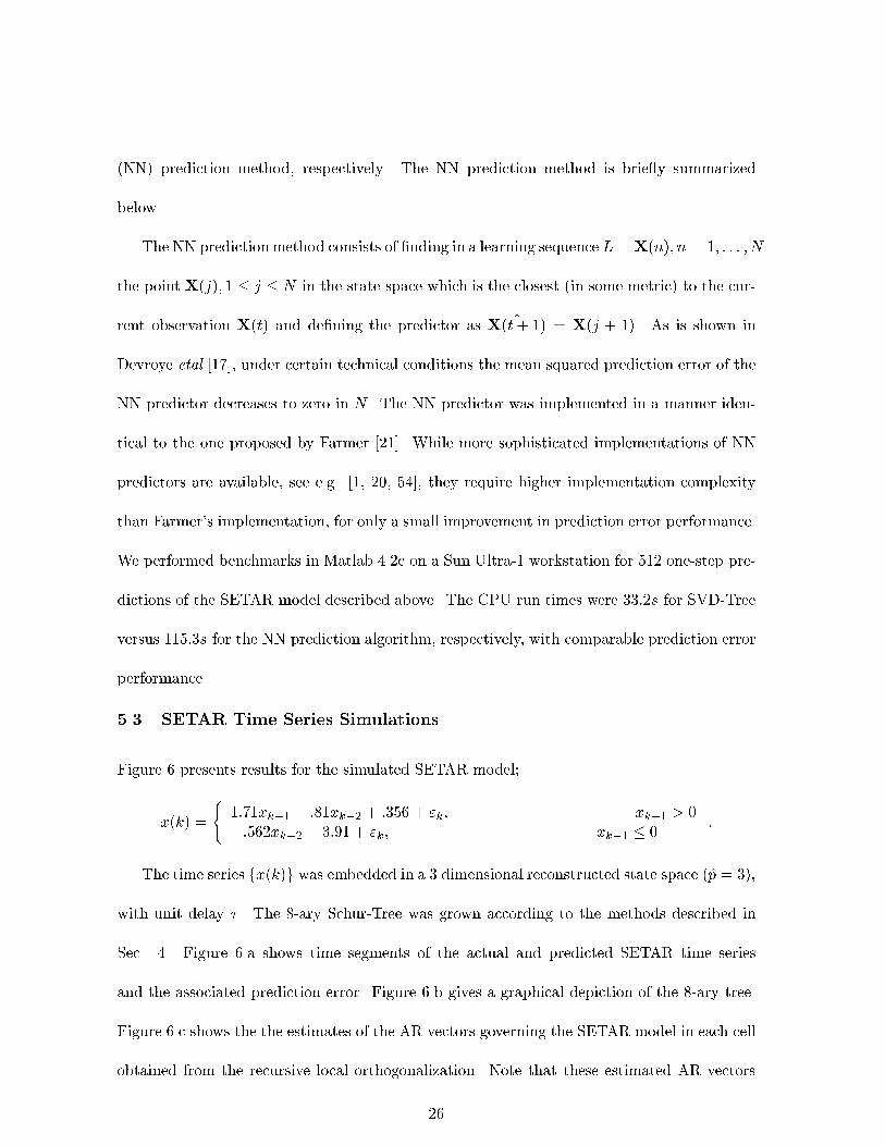
(NN) prediction method, respectively. The NN prediction method is brie y summarized

below.

The NN prediction method consists of �nding in a learning sequence L = X(n); n = 1; : : : ; N

the point X(j); 1 � j � N in the state space which is the closest (in some metric) to the cur-

rent observation X(t) and de�ning the predictor as ^X(t+ 1) = X(j + 1). As is shown in

Devroye etal [17], under certain technical conditions the mean squared prediction error of the

NN predictor decreases to zero in N . The NN predictor was implemented in a manner iden-

tical to the one proposed by Farmer [21]. While more sophisticated implementations of NN

predictors are available, see e.g. [1, 20, 54], they require higher implementation complexity

than Farmer's implementation, for only a small improvement in prediction error performance.

We performed benchmarks in Matlab 4.2c on a Sun Ultra-1 workstation for 512 one-step pre-

dictions of the SETAR model described above. The CPU run times were 33:2s for SVD-Tree

versus 115:3s for the NN prediction algorithm, respectively, with comparable prediction error

performance.

5.3 SETAR Time Series Simulations

Figure 6 presents results for the simulated SETAR model;

x(k) =

(1:71xk�1 � :81xk�2 + :356 + "k; xk�1 > 0�:562xk�2 � 3:91 + "k; xk�1 � 0

:

The time series fx(k)g was embedded in a 3 dimensional reconstructed state space (p = 3),

with unit delay � . The 8-ary Schur-Tree was grown according to the methods described in

Sec. 4. Figure 6.a shows time segments of the actual and predicted SETAR time series

and the associated prediction error. Figure 6.b gives a graphical depiction of the 8-ary tree.

Figure 6.c shows the the estimates of the AR vectors governing the SETAR model in each cell

obtained from the recursive local orthogonalization. Note that these estimated AR vectors

26

cluster in two directions which closely correspond to the two AR(2) regimes of the actual

SETAR model (5.3).

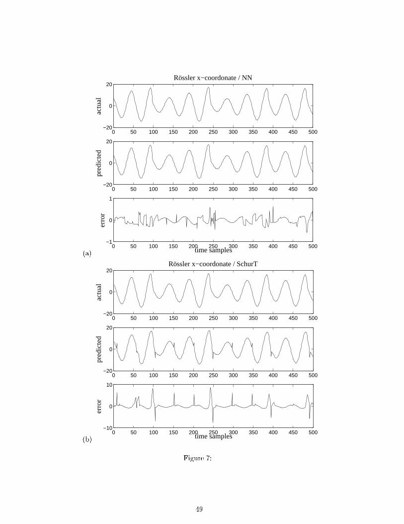
5.4 R�ossler Simulations

The discrete time R�ossler system generates a chaotic measurement x(t) generated by the

non-linear set of di�erential equations :8><>:dxdt = �y � zdydt = �x+ aydzdt = b+ xz � cz

(19)

where x; y; z are components of the three dimensional state vector of the R�ossler system.

We simulated (19) using the following set of parameter values: a = 0; 15, b = 0; 2 et c = 10.

The set of non linear coupled ordinary di�erential equations were numerically integrated, using

an order 3 Runge-Kutta approach. The recorded time series correspond to the �rst coordinate

(x(t)) of the system, sampled at a period h = :4s 2

The reconstruction dimension was varied from 2 to 5, but the reconstruction delay is

maintained to a constant value � = 4h. The prediction error variance is estimated from N

predicted values by

V =

PNi=1(ei � ei)

2PNi=1(xi � xi)2

:

The Schur tree was grown from phase space time series of duration N=500 and the

training set consisted of 8192 phase space state vectors. Figure 7 shows the one-step forward

prediction and errors for NN and Schur-Tree methods applied to the R�ossler time series. Note

that both NN and Schur-Tree predictors have similar trajectories although the more complex

NN implementation achieves somewhat smaller prediction error. The spikes observed in the

Schur-Tree prediction residuals are due to transitions between the local models in phase space.

2For simulating this chaotic system by numerically integrating this set of ordinary di�erential equations,

h must be set to a much smaller value than the sampling step of the recorded time series, in order to avoid

numerical instabilities. The integration was performed with a time increment h0 = h=64

27

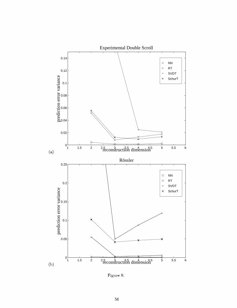
5.5 Algorithm Comparisons

A comparison of the performance of the four di�erent one-step forward prediction methods

discussed in this paper is illustrated in Figure 8 for the Chua circuit measurements and the

R�ossler simulation. The four methods studied are: the tree-structured predictor of Sec. 3.3

(RT), the SVD-Tree and the Schur-Tree discussed in Sec. 4, and the nearest neighbor (NN)

algorithm. Note the relative performance advantage of the recursive Schur-Tree as compared

to the SVD-Tree. We believe that this is due to the instability of the AR model obtained

from SVD-Tree; the Schur-Tree is guaranteed to give a stable model. In all the cases the NN

algorithm slightly outperforms the tree-based methods, but the improvement is obtained at

a signi�cant increase in computational burden.

6 Conclusions

We have presented a low complexity algorithm based on recursive state space partitioning

for performing near-optimal non-linear prediction and identi�cation of non-linear signals. We

have also derived local SVD and Schur decomposition versions which are naturally suited to

piecewise constant AR models (SETAR). These algorithms were numerically illustrated for

simulated SETARmeasurements, simulated chaotic measurements, and voltage measurements

obtained from a Chua electronic circuit.

The tree based prediction approach presented here is related to the classi�cation and re-

gression tree (CART) technique [9] and adaptive tree structured vector quantization (TSVQ)

[14]. The main di�erence is our use of a locally de�ned recursive SVD orthogonalization and

its intrinsic applicability to piecewise linear generalizations of thresholded AR (SETAR) mod-

els [61]. Our tree-structure with SVD orthogonalization is also related to (unitary) transform

coding [27], the di�erence being that the orthogonalization is applied locally and recursively

28

to each splitting node. Future work will include detection of the local linearized dynamics

and regularization for smoothing out model discontinuity between partition cells. A related

issue for future study is how to deal with larger values of the imbedding dimension p. The

2p-ary splitting rule proposed here produces subcells of equal volume but gives a model with

complexity, i.e. the number of free parameters, exponential in p. Therefore, to avoid the

need for unreasonably large amounts of training data p must be held as small as possible

without sacri�cing quantization error performance. A reasonable alternative would be to use

the standard binary splitting rule for growing the model; restricting the 2p splitting rule to

implementation of the subcell uniformity tests.

29

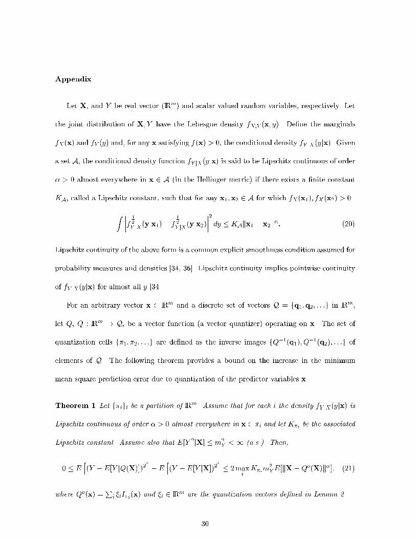
Appendix

Let X, and Y be real vector (IRm) and scalar valued random variables, respectively. Let

the joint distribution of X; Y have the Lebesgue density fX;Y (x; y). De�ne the marginals

fX(x) and fY (y) and, for any x satisfying f(x) > 0, the conditional density fY jX(yjx). Given

a set A, the conditional density function fY jX(yjx) is said to be Lipschitz continuous of order

� > 0 almost everywhere in x 2 A (in the Hellinger metric) if there exists a �nite constant

KA, called a Lipschitz constant, such that for any x1;x2 2 A for which fX(x1); fX(x2) > 0

Z ����f 1

2

Y jX(yjx1)� f1

2

Y jX(yjx2)����2 dy � KAkx1 � x2k�: (20)

Lipschitz continuity of the above form is a common explicit smoothness condition assumed for

probability measures and densities [34, 36]. Lipschitz continuity implies pointwise continuity

of fY jX(yjx) for almost all y [34].

For an arbitrary vector x 2 IRm and a discrete set of vectors Q = fq1;q2; : : :g in IRm,

let Q, Q : IRm ! Q, be a vector function (a vector quantizer) operating on x. The set of

quantization cells f�1; �2; : : :g are de�ned as the inverse images fQ�1(q1); Q�1(q2); : : :g of

elements of Q. The following theorem provides a bound on the increase in the minimum

mean square prediction error due to quantization of the predictor variables x.

Theorem 1 Let f�igi be a partition of IRm. Assume that for each i the density fY jX(yjx) is

Lipschitz continuous of order � > 0 almost everywhere in x 2 �i and let K�i be the associated

Lipschitz constant. Assume also that E[Y 2jX] � m2Y <1 (a.s.). Then,

0 � Eh(Y �E[Y jQ(X)])2

i�E

h(Y �E[Y jX])2

i� 2max

iK�im

2YE[kX�Qo(X)k�]: (21)

where Qo(x) =P

i �iI�i(x) and �i 2 IRm are the quantization vectors de�ned in Lemma 2.

30

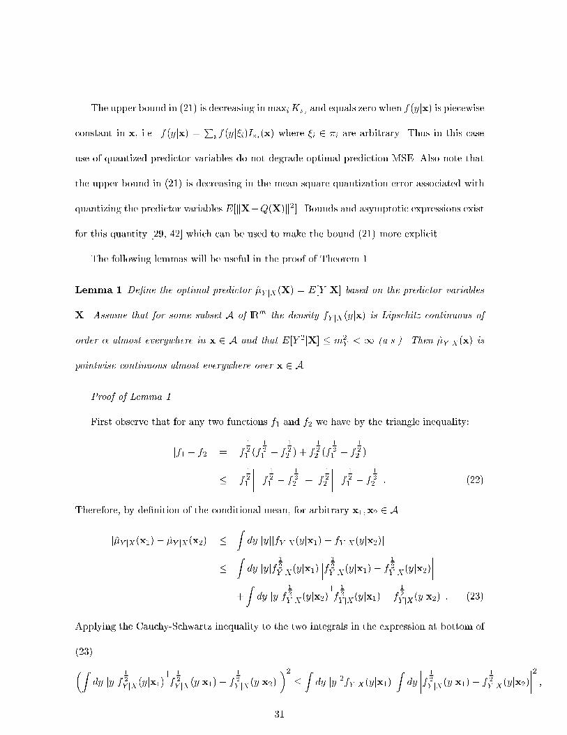
The upper bound in (21) is decreasing in maxiK�i and equals zero when f(yjx) is piecewise

constant in x, i.e. f(yjx) = Pi f(yj�i)I�i(x) where �i 2 �i are arbitrary. Thus in this case

use of quantized predictor variables do not degrade optimal prediction MSE. Also note that

the upper bound in (21) is decreasing in the mean square quantization error associated with

quantizing the predictor variables E[kX�Q(X)k2]. Bounds and asymptotic expressions exist

for this quantity [29, 42] which can be used to make the bound (21) more explicit.

The following lemmas will be useful in the proof of Theorem 1.

Lemma 1 De�ne the optimal predictor �Y jX(X) = E[Y jX] based on the predictor variables

X. Assume that for some subset A of IRm the density fY jX(yjx) is Lipschitz continuous of

order � almost everywhere in x 2 A and that E[Y 2jX] � m2Y < 1 (a.s.). Then �Y jX(x) is

pointwise continuous almost everywhere over x 2 A.

Proof of Lemma 1

First observe that for any two functions f1 and f2 we have by the triangle inequality:

jf1 � f2j =

����f 1

2

1 (f1

2

1 � f1

2

2 ) + f1

2

2 (f1

2

1 � f1

2

2 )

�����

����f 1

2

1

���� ����f 1

2

1 � f1

2

2

����+ ����f 1

2

2

���� ����f 1

2

1 � f1

2

2

���� : (22)

Therefore, by de�nition of the conditional mean, for arbitrary x1;x2 2 A

j�Y jX(x1)� �Y jX(x2)j �Zdy jyjjfY jX(yjx1)� fY jX(yjx2)j

�Zdy jyjf

1

2

Y jX(yjx1)����f 1

2

Y jX(yjx1)� f1

2

Y jX(yjx2)����

+

Zdy jyjf

1

2

Y jX(yjx2)����f 1

2

Y jX(yjx1)� f1

2

Y jX(yjx2)���� : (23)

Applying the Cauchy-Schwartz inequality to the two integrals in the expression at bottom of

(23)�Zdy jyjf

1

2

Y jX(yjx1)����f 1

2

Y jX(yjx1)� f1

2

Y jX(yjx2)�����2

�Zdy jyj2fY jX(yjx1)

Zdy

����f 1

2

Y jX(yjx1)� f1

2

Y jX(yjx2)����2 ;

31

and similarly for the second integral. Hence, Lipschitz continuity of fY jX(yjx) over x 2 A

gives the bound

j�Y jX(x1)� �Y jX(x2)j2 � 2maxx

E[y2jx]Zdy

����f 1

2

Y jX(yjx1)� f1

2

Y jX(yjx2)����2

� 2m2YKAkx1 � x2k�; (24)

where KA <1 is the associated Lipschitz constant. This establishes the lemma. 2

Lemma 2 De�ne the optimal predictor �Y jQ(x) = E[Y jQ(X)] based on quantized predictor

variables Q(X). Assume that fY jX(yjx) is Lipschitz continuous of order � almost everywhere

in x 2 �i and that E[Y 2jX] � m2Y <1 (a.s.). Then for any quantization cell �i � IRm there

exists a point �i 2 �i such that

�Y jQ(x) = �Y jX(�i); 8x 2 �i:

Furthermore, the point �i satis�es the equation

Z�i

dx �Y jX(x)f(x) = �Y jX(�i)PX(�i);

where PX(�i) =R�if(x)dx.

Proof of Lemma 2

By de�nition of conditional expectation: �Y jQ(x) =Rdy yfY jQ(yjQ(x)) where

fY jQ(yjQ(x)) =Z�idx fY jX(yjx)f(x)=PX (�i); x 2 �i

is the conditional density of Y given Q(X) = Q(x). Invoking Fubini's theorem [53] to permute

the order of integration, we obtain the Lebesgque-Steiltjes integral representation

�Y jQ(x) =1

PX(�i)

Z�idx f(x)

Zdy yfY jX(yjx)

=1

PX(�i)

Z�i

dP (x) �Y jX(x); x 2 �i

32

where dP (x) = f(x)dx. By Lemma 1 �Y jX(x) is continuous and therefore, by the mean value

theorem for Lebesgue-Steiltjes integrals [53], there exists a point �i 2 �i such that

1

PX(�i)

Z�idP (x)�Y jX(x) = �Y jX(�i); x 2 �i:

This establishes the Lemma. 2

Proof of Theorem 1

De�ne

�2 def= E

h(Y �E[Y jQ(X)])2

i�E

h(Y �E[Y jX])2

i:

That �2 > 0 follows directly from the fact that the conditional mean estimator E[Y jX] min-

imizes mean square prediction error. Next we deal with the right hand side of the inequality

(21). It is easily veri�ed by iterated expectation that E [(Y �E[Y jQ(X)])E[Y jQ(X)]] = 0 and

E [(Y �E[Y jX])E[Y jX]] = 0 (orthogonality principle of non-linear estimation). Therefore

�2 = E [(Y �E[Y jQ(X)])Y ]�E [(Y �E[Y jX])Y ]

= E [(E[Y jX]�E[Y jQ(X)]) Y ]

= E [(E[Y jX]�E[Y jQ(X)])E[Y jX]] :

Thus, by Fubini [8], we have the integral representation

�2 =

Zdx

h�Y jX(x) � �Y jQ(x)

i�Y jX(x)f(x)

=Xi

Z�idx

h�Y jX(x)� �Y jQ(x)

i�Y jX(x)f(x); (25)

where the � quantities are de�ned as in Lemmas 1 and 2. Invoking the latter lemma, there ex-

ists a point �i 2 �i such that �Y jQ(x) = �Y jX(�i), x 2 �i andR�idx [�Y jX(x)��Y jX(�i)]f(x) =

0. Therefore, from (25)

�2 =Xi

Z�i

dx����Y jX(x)� �Y jX(�i)

���2 f(x):33

Application of the bound (24) on j�Y jX(x1) � �Y jX(x2)j2 obtained in the course of proving

Lemma 1 yields

�2 � 2m2Y max

iK�i

Xi

Z�i

dx kx� �ik�f(x)

= 2m2Y max

iK�i E [kX�Qo(X)k�]

where Qo(x) =P

i �iI�i(x). 2

34

References

[1] H.Abarbanel, R.Brown, J.Sidorowitch, L.Tsimring, \ The Analysis of Observed Chaotic

Data in Physical Systems",Rev. Mod. Phys., vol.65(4), pp.1331-1391, 1990.

[2] H. Abarbanel, \Analysis of Observed Chaotic Data," Institute for Nonlinear Science,

Springer-Verlag, NY 1996.

[3] M. Abromowitz and I. Stegun, \Handbook of Mathematical Functions," Dover, New

York, NY, 1977.

[4] M. Basseville, \Distances Measures for Signal Processing and Pattern Recognition", Sig-

nal Processing, vol.18, pp 349-369.

[5] J. Bentley, \Multidimensional binary search trees used for associative searching," Com-

munic. Assoc. Comput. Mach., vol. 18, pp. 509{517, 1975.

[6] A.E. Badel, O. Michel, A.O. Hero, \ Arbres de R�egression : Mod�elisation Non

Param�etrique et Analyse des S�eries Temporelles" Revue de Traitement du Signal, Vol.

14, No. 2, pp. 117-133, June 1997.

[7] P. J. Bickel and K. A. Doksum, \Mathematical Statistics: Basic Ideas and Selected

Topics", Holden-Day, San Francisco (CA), 1977.

[8] P. Billingsley, Probability and Measure, Wiley, New York, 1979.

[9] L. Breiman, J.H.Friedman, R.A. Olshen, C.J. Stone, \Classi�cation and Regression

Trees," Wadsworth Advanced Books and Software, 1984.

35

[10] A.E. Badel, L. Mercier, D. Guegan, O. Michel, \Comparison of several methods to predict

chaotic time series.", Proceedings of IEEE-ICASSP'97, Munich, Vol.V, pp.3793-3796,

April 1997.

[11] M. Casdagli, T. Sauer, J.A Yorke, \Embedology", J. Stat. Phys, vol.65, 1991, pp.579-616

[12] \Nonlinear Modeling and Forecasting", M. Casdagli and S. Eubank Ed., Proceedings

Volume in the Santa Fe Institute Studies for the Sciences of Complexity, Vol. 12, 1991.

[13] L. Clarke and D. Pregibon, \Tree-based models," in Statistical Models in S, J. Chambers

and T. Hastie, editors, pp. pp. 377{419, Wadsworth, 1992.

[14] P.A. Chou, T. Lookabaugh, R.M. Gray, \Optimal Pruning with Applications to Tree-

Structures Source Coding and Modeling," IEEE Trans on Inf. theory, vol.35, No.2, pp

299-315, 1989.

[15] W. Cleveland, E. Grosse, and W. Shyu, \Local regression models," in Statistical Models

in S, J. Chambers and T. Hastie, editors, pp. pp. 309{376, Wadsworth, 1992.

[16] H. A. David, \Order Statistics", Wiley, New York, 1981.

[17] L.Devroye, L�asl�o Gy�or�, G�abor Lugosi, \ A Probabilistic Theory of Pattern Recogni-

tion", Application of Math. Series, vol.31, Springer Verlag, 1996.

[18] R.F. Engle, \Autoregressive conditional heteroscedasticity with estimates of the variance

of United Kingdom in ation", Econometrica, vol.50, pp.987-1007, 1982.

[19] J.P. Eckmann and D. Ruelle, \Ergodic Theory of Chaos and Strange Attractors," Rev.

Mod. Phys., Vol. 57, No. 3, pp. 617{656, 1985.

36

[20] J.D.Farmer, J.Sidorowitch, \ Predicting Chaotic Time Series", Phys. Rev. Lett., 59:845,

1987

[21] J.D.Farmer, J.Sidorowitch, \Exploiting Chaos to Predict the Future and Reduce Noise",

in Evolution, Learning and Cognition, Y.C.Lee Ed., World Scienti�c, Singapore 1988,

277-330.

[22] A.M. Fraser, \Information and Entropy in Strange Attractors," IEEE Trans on Inf.

theory, vol.35, No.2, pp 245-262, 1989.

[23] A.M. Fraser, H.L. Swinney, \Independent Coordinates for Strange Attractors from Mu-

tual Information," Phys. Rev. A, Vol.33, No.2, pp.1134-1140, 1981.

[24] A.M. Fraser, \Modeling NonLinear TimeSeries," ICASSP'92, vol.5 San Francisco, 1992,

pp.V313-V317.

[25] A.M. Fraser, A. Dimitriadis, \Forecasting Probability Densisty by Using Hidden Markov

Models with mixed States," Time Series Prediction, A.S. Weigend, N.A.Gershenfeld ed.,

Proceeding volume of the Santa Fe institute, vol.XV, pp.265-282.

[26] K. Fukunaga, \Statistical Pattern Recognition (2nd Ed), Academic Press, San Diego

(CA), 1990.

[27] A. Gersho, R.M. Gray, \Vector Quantization and Signal Compression", Kluwer Academic

Press, 1992.

[28] P.Grassberger, I.Procaccia, \Measuring the Strangeness of Strange Attractors," Physica

D, Vol.9, pp.189-208, 1983.

[29] R. M. Gray, Source Coding Theory, Kluwer Academic, Norwell MA, 1990.

37

[30] D.Guegan, \On the identi�cation and prediction of nonlinear models", Proceedings of

the Workshop on New Directions in Time Series Analysis, Springer Verlag, 1992.

[31] D.Guegan, S�eries Chronologiques Non Lin�eaires �a temps discret," Statistique

Math�ematique et Probabilit�e, Economica, Paris, 1994.

[32] S.Haykin, J.Principe \Using neural networks to dynamically model chaotic events such

as sea clutter; Making sense of a complex world", IEEE Signal Processing Magazine,

66:81, Mai 1998.

[33] D.R.Hush, B.G.Horne \ Progress in Supervised Neural Networks", Signal Processing

Magazine, IEEE, 8:38, janvier 1993.

[34] I. A. Ibragimov and R. Z. Has'minskii, Statistical estimation: Asymptotic theory,

Springer-Verlag, New York, 1981.

[35] H. Kantz and T.Schreiber, \Nonlinear Time Series Analysis", Cambridge Nonlinear Sci-

ence Series 7, Cambridge University Press 1997.

[36] L. LeCam, Asymptotic Methods in Statistical Decision Theory, Springer-Verlag, New

York, 1986.

[37] E.L. Lehmann, \Testing Statistical Hypotheses", Wiley, New York, 1959.

[38] W. Liebert, K. Pawelzik, H.G. Schuster, \ Optimal embedding of Chaotic Attractors

from topological Considerations", Europhysics Letters, Vol.14, No.6, pp.521-526, 1991.

[39] A. Mead, R.D. Jones et al., \Prediction of Chaotic Time Series Using CNLS-Net-

Example: The mackey-Glass Equation,", in \Nonlinear Modeling and Forecasting",

38

M.Casdagli and S.Eubank Ed., Proc. of the Santa Fe Institute vol.12, Addison Wes-

ley, 1992, pp.39-72. .

[40] O. Michel, P. Flandrin, \Higher Order Statistics For Chaotic Signal Processing," Control

and Dynamic Systems, Vol.75, pp.105-153, Academic Press, 1996.

[41] A.M. Mood, F.A. Graybill, D.C. Boes, \Introduction to the Theory of Statistics," Mc

Graw Hill International Editions, Statistics Series, 3rd ed. 1974.

[42] D. N. Neuho�, \On the asymptotic distribution of the errors in vector quantization,"

IEEE Trans. on Inform. Theory, vol. IT-42, pp. 461{468, March 1996.

[43] A. Nobel, \Vanishing distortion and shrinking cells," IEEE Trans. on Inform. Theory,

vol. IT-42, no. 4, pp. 1303{1305, 1996.

[44] A. Nobel, \Recursive partitioning to reduce distortion," IEEE Trans. on Inform. Theory,

vol. IT-43, no. 4, pp. 1122{1133, 1997.

[45] A. Nobel and R. Olshen, \Termination and continuity of greedy growing for tree-

structured vector quantizers," IEEE Trans. on Inform. Theory, vol. IT-42, no. 1, pp.

191{205, 1996.

[46] M. Orchard and C. Bouman, \Color quantization of images," IEEE Trans. on Signal

Processing, vol. SP-39, no. 12, pp. 2677{2690, 1991.

[47] K. Perlmutter, S. Perlmutter, R. Gray, R. Olshen, and K. Oehler, \Bayes risk weighted

vector quantization with posterior estimation for image compression and classi�cation,"

IEEE Trans. on Image Processing, vol. IP-5, no. 2, pp. 347{360, 1996.

39

[48] A. Papoulis, \Probability, Random Variables, and Stochastic Processes", McGraw-Hill

Int. Editions, 2nd edition, 1984.

[49] T. S. Parker, L. O. Chua, \Practical Numerical Algorithms for Chaotic Systems",

Springer Verlag, 1989.

[50] W.H. Press, B.P. Flannery, S.A. Teukolsky, W.T. Vetterling, \Numerical recipes in C",

Cambridge University Press, 1989.

[51] M.B. Priestley, \State Dependant models: a general approach to nonlinear time series

analysis", Journal of Time Series Analysis, vol.1, pp.47-71, 1980.

[52] M.B. Priestley, \Non Linear and Non Stationary Time Series Analysis," Academic Press,

San Diego, 1988.

[53] F. Riesz and B. Sz.-Nagy, Functional analysis, Ungar, New York, 1955.

[54] T. Sauer, \A noise reduction method for signal from nonlinear systems.", Physica D,

vol.58, pp.193-201, 1992.

[55] M.R. Segal, \Tree structured methods for longitudinal data," Journ. Amer. Stat. Assoc.

(JASA), vol. 87, pp. 407-418, May 1992.

[56] L. L. Scharf, \Statistical Signal Processing, Detection, Estimation and Time Series Anal-

ysis", Addison-Wesley Pub. Co., 1990.

[57] R. Shaw, \Strange Attractors, Chaotic Behavior and Information Flow", in Zeitschrift

in NaturForschung, vol.36A, No.1, pp.80-112, 1981.

[58] J.N. Sonquist and J.N. Morgan, \The detection of interaction e�ects," Monograph 35,

Survey Research Center, Institute for Social Research, University of Michigan, 1964.

40

[59] F. Takens, \Detecting Strange Attractors in Turbulence," Lecture Notes in Mathematics,

Vol.898, pp.366-381, 1981.

[60] H. Tong \Threhold models in nonlinear time series analysis", Lecture Notes in Statistics,

vol.21, Springer Verlag, 1983.

[61] H. Tong, \Non Linear Time Series : a Dynamical system Approach," Oxford Science

Publication, Oxford University Press, NY 1990.

[62] G.Wahba, \Multivariate Function and Operator Estimation, Based on Smoothing Splines

and Reproducing Kernels," in \Nonlinear Modeling and Forecasting", M.Casdagli and

S.Eubank Ed., Proc. of the Santa Fe Institute vol.12, Addison Wesley, 1992, pp.95-112.

[63] T.P. Weldon, \An Inductorless Double-Scroll Chaotic Circuit", American Journal of

Physics, vol. 58, No.10, pp.936-941, 1990.

[64] \Time Series Prediction : Forecasting the Future and Understanding the Past",

A.S.Weigend and N.A.Gershenfeld Ed., Proceedings Volume in the Santa Fe Institute

Studies for the Sciences of Complexity, Vol. 15, 1992.

[65] H. Whitney, \Di�erentiable Manifolds", Annals of Mathematics, Vol.37 No.3, pp.645-680,

1936.

[66] H. Zhang, \ Classi�cationtrees for multiple binary responses," Journ. Amer. Stat. Assoc.

(JASA), vol. 93, No. 441, pp 180-193, Mar. 1998.

41

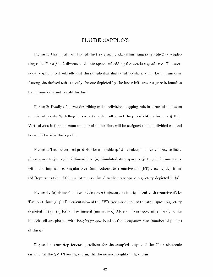
FIGURE CAPTIONS

Figure 1: Graphical depiction of the tree growing algorithm using separable 2p-ary split-

ting rule. For a p = 2 dimensional state space embedding the tree is a quad-tree. The root-

node is split into 4 subcells and the sample distribution of points is found be non-uniform.

Among the derived subsets, only the one depicted by the lower left corner square is found to

be non-uniform and is split further.

Figure 2: Family of curves describing cell subdivision stopping rule in terms of minimum

number of points N� falling into a rectangular cell � and the probability criterion � 2 [0; 1].

Vertical axis is the minimum number of points that will be assigned to a subdivided cell and

horizontal axis is the log of �.

Figure 3: Tree-structured predictor for separable splitting rule applied to a piecewise linear

phase space trajectory in 2 dimensions. (a) Simulated state space trajectory in 2 dimensions,

with superimposed rectangular partition produced by recursive tree (RT) growing algorithm.

(b) Representation of the quad-tree associated to the state space trajectory depicted in (a).

Figure 4 : (a) Same simulated state space trajectory as in Fig. 3 but with recursive SVD-

Tree partitioning. (b) Representation of the SVD-tree associated to the state space trajectory

depicted in (a). (c) Pairs of estimated (normalized) AR coe�cients governing the dynamics

in each cell are plotted with lengths proportional to the occupancy rate (number of points)

of the cell.

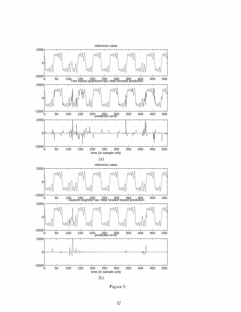
Figure 5 : One step forward predictor for the sampled output of the Chua electronic

circuit: (a) the SVD-Tree algorithm; (b) the nearest neighbor algorithm.

42

Figure 6: SETAR time series from equation (5.3): (a) one step forward predictor trajectory

and prediction errors obtained from Schur-Tree algorithm; (b) 8-ary tree constructed from

a 3 dimensional state phase space using Schur-Tree algorithm; (c) unit-length AR direction

vectors.

Figure 8: Normalized prediction error variance as a function of the reconstruction dimen-

sion for: (a) the voltage output of a Chua electronic circuit; and (b) the simulated R�ossler

time series.

Figure 7: simulated time series, one step forward predicted values and prediction errors for

the �rst coordinate of the R�ossler system (p = 3) using: (a) NN algorithm; and (b) Schur-Tree

algorithm.

43

xxxxxxxxx

x x xxx

x xxx xxxxx x xxxx xx

x xxx x x Depth ‘0’<=> Root Node

Depth‘1’

Depth ‘2’

Figure 1:

p=1

p=3

p=5

p=7

p=9

10−8

10−6

10−4

10−2

100

0

5

10

15

20

25

30

35

log(epsilon)

Min

imum

num

ber

of p

oint

s pe

r ce

ll

Stopping Criterion: Exact Under Gaussian Approximation

Figure 2:

44

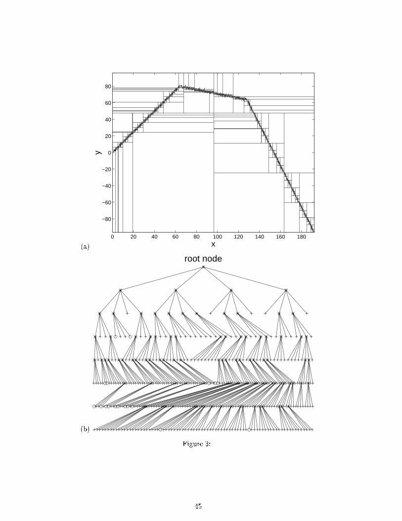
(a)

0 20 40 60 80 100 120 140 160 180

−80

−60

−40

−20

0

20

40

60

80

x

y

(b)

root node

Figure 3:

45

(a)

0 50 100 150

−80

−60

−40

−20

0

20

40

60

80

x

y

(b)

root node

(c)−0.5 −0.4 −0.3 −0.2 −0.1 0 0.1 0.2 0.3 0.4 0.5

−0.5

−0.4

−0.3

−0.2

−0.1

0

0.1

0.2

0.3

0.4

0.5

A1

A2

Figure 4:

46

0 50 100 150 200 250 300 350 400 450 500−2000

0

2000reference value

0 50 100 150 200 250 300 350 400 450 500−2000

0

2000 Tree based quantized tau−step forward prediction

0 50 100 150 200 250 300 350 400 450 500−2000

0

2000

time (in sample unit)

prediction error

(a)

0 50 100 150 200 250 300 350 400 450 500−2000

0

2000reference value

0 50 100 150 200 250 300 350 400 450 500−2000

0

2000 nearest neighbor tau−step forward based prediction

0 50 100 150 200 250 300 350 400 450 500−2000

0

2000

time (in sample unit)

prediction error

(b)

Figure 5:

47

(a)

0 50 100 150 200 250 300 350 400 450 500−20

0

20Bimodal SETAR Time Series

actu

al

0 50 100 150 200 250 300 350 400 450 500−20

0

20

pred

icte

d

0 50 100 150 200 250 300 350 400 450 500−10

0

10

erro

r

time samples (b)

Root Node

(c)−0.1

−0.050

0.050.1

−0.1

−0.05

0

0.05

0.1−0.1

−0.05

0

0.05

0.1

A1A2

A3

Figure 6:

48

(a)

0 50 100 150 200 250 300 350 400 450 500−20

0

20

pred

icte

d

0 50 100 150 200 250 300 350 400 450 500−1

0

1

erro

r

time samples

0 50 100 150 200 250 300 350 400 450 500−20

0

20

actu

al

Rossler x−coordonate / NN

(b)

0 50 100 150 200 250 300 350 400 450 500−20

0

20Rossler x−coordonate / SchurT

actu

al

0 50 100 150 200 250 300 350 400 450 500−20

0

20

pred

icte

d

0 50 100 150 200 250 300 350 400 450 500−10

0

10

erro

r

time samples

Figure 7:

49

(a)

NN

RT

SVDT

SchurT

1 1.5 2 2.5 3 3.5 4 4.5 5 5.5 60

0.02

0.04

0.06

0.08

0.1

0.12

0.14pr

edic

tion

erro

r va

rianc

e

reconstruction dimension

Experimental Double Scroll

(b)

NN

RT

SVDT

SchurT

1 1.5 2 2.5 3 3.5 4 4.5 5 5.5 60

0.05

0.1

0.15

0.2

0.25

pred

ictio

n er

ror

varia

nce

reconstruction dimension

Rossler

Figure 8:

50

Biographies

ALFRED O. HERO, III, (S '79, M '84, SM '96, F '97) was born in Boston, MA, USA

in 1955. He received the B.S. (summa cum laude) from Boston University (1980) and the

Ph.D. from Princeton University (1984), both in electrical engineering. He held the G.V.N.

Lothrop Fellowship in Engineering at Princeton University. Since 1984 Alfred Hero has been

with the Dept. of Electrical Engineering and Computer Science, University of Michigan -

Ann Arbor, where he is currently Professor and Director of the Communications and Signal

Processing Laboratory. He has held positions of Visiting Scientist at MIT Lincoln Laboratory,

Lexington, MA (1987-89); Visiting Professor at l'Ecole Nationale de Techniques Avancees

(ENSTA), Paris, France (1991); and William Clay Ford Fellow at the Ford Motor Company,

Dearborn, MI (1993). He has served as consultant for US government agencies and private

industry. His present research interests are in the areas of detection and estimation theory,

statistical signal and image processing, statistical pattern recognition, signal processing for

communications, channel equalization and interference mitigation, spatio-temporal sonar and

radar processing, and biomedical signal and image analysis.

Alfred Hero is a Fellow of the IEEE, a member of Tau Beta Pi, the American Statistical

Association, the New York Academy of Science, and Commission C of the International

Union of Radio Science (URSI). In 1995 he received a Research Excellence Award from the

College of Engineering at the University of Michigan. In 1999 he received a Best Paper

Award from the IEEE Signal Processing Society. He was associate editor for the IEEE

Transactions on Information Theory (1994-97); Chair of the IEEE SPS Statistical Signal and

Array Processing Technical Committee (1996-98); and Treasurer of the IEEE SPS Conference

Board (1997-2000). He was co-chair for the 1999 IEEE Information Theory Workshop and

51

the 1999 IEEE Workshop on Higher Order Statistics. He served as publicity chair for the

1986 IEEE International Symposium on Information Theory and was general chair of the 1995

IEEE International Conference on Acoustics, Speech, and Signal Processing. He received the

1999 Meritorious Service Award from the IEEE Signal Processing Society.

OLIVIER J.J.MICHEL (S'84, M'85) was born in Mont Saint Martin, France, in 1963. He

completed his studies at Ecole Normale Sup�erieure de Cachan, in the department of Applied

Physics, where he received the \Agr�egation de Physique" in 86. He received a Ph.D degree

from University Paris-XI Orsay in 91, in signal processing. In 91, he joined the physics

department at Ecole Normale Sup�erieure de Lyon, France, as an assistant professor. His

research interest include non stationnary spectral analysis, array processing, non linear time

series problems, information theory and dynamical systems studies, in close relationship with

physical experiments in the �eld of chaos and hydrodynamical turbulence.

ANNE EMMANUELLE BADEL (S'92, M'93) was born in Lyon, France, in 1971. She

completed her studies at Ecole Normale Sup�erieure de Lyon, France, in the physics depart-

ment. She completed the Agr�gation de Physique in 1994, and completed a PhD in Physics

at ENS-Lyon in 1998. Her research interests are in non linear time series analysis. in Physics

in 1998, at ENS-Lyon.

52