1

Instruction-Level Parallelism

CS448

2

Instruction Level Parallelism (ILP)

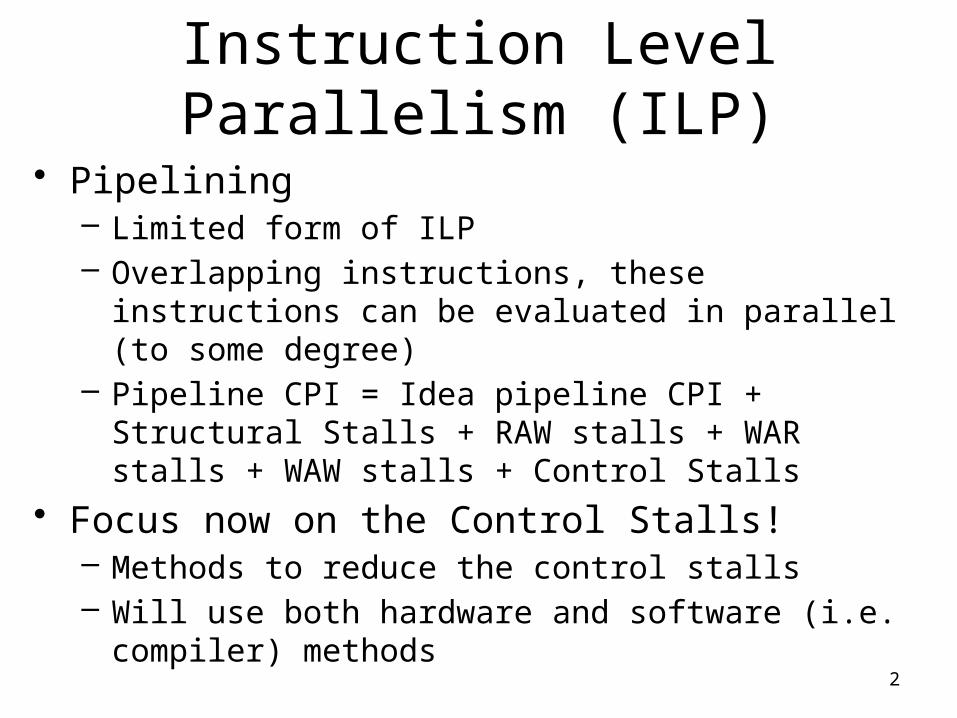
• Pipelining – Limited form of ILP– Overlapping instructions, these instructions can be evaluated in

parallel (to some degree)– Pipeline CPI = Idea pipeline CPI + Structural Stalls + RAW

stalls + WAR stalls + WAW stalls + Control Stalls

• Focus now on the Control Stalls!– Methods to reduce the control stalls– Will use both hardware and software (i.e. compiler) methods

3

Techniques

4

ILP and Basic Blocks

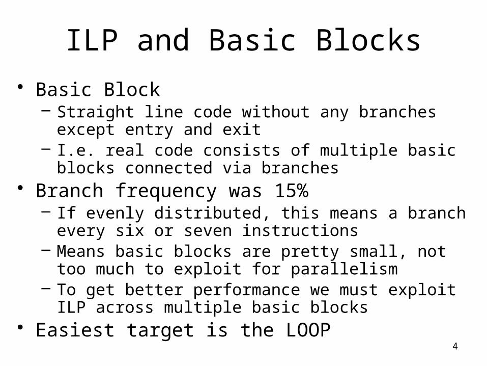
• Basic Block– Straight line code without any branches except entry and exit– I.e. real code consists of multiple basic blocks connected via

branches• Branch frequency was 15%

– If evenly distributed, this means a branch every six or seven instructions

– Means basic blocks are pretty small, not too much to exploit for parallelism

– To get better performance we must exploit ILP across multiple basic blocks

• Easiest target is the LOOP

5

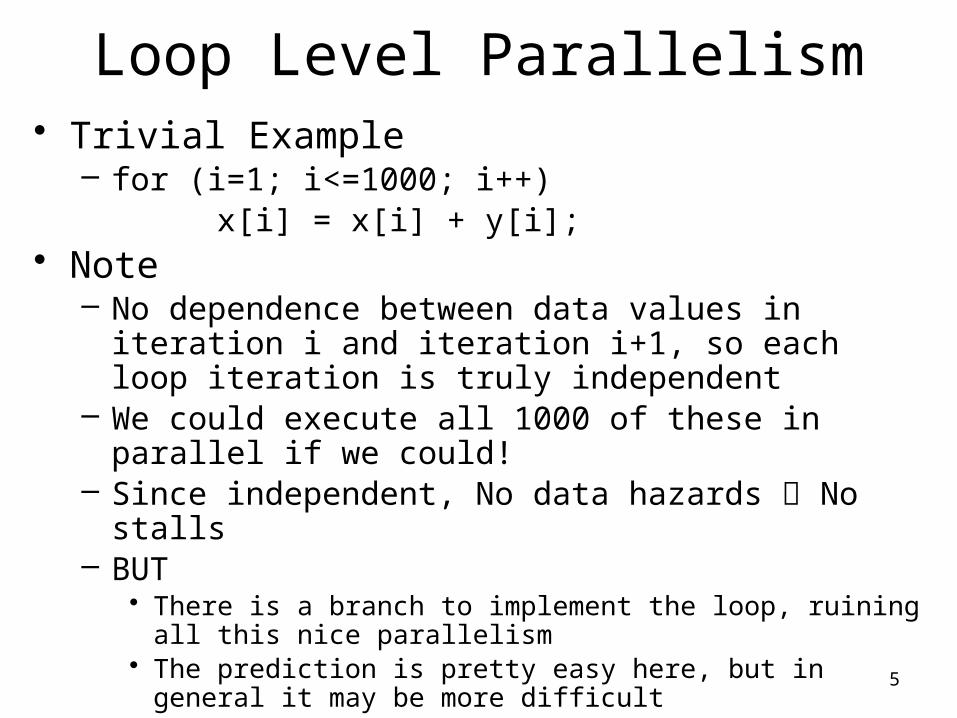
Loop Level Parallelism• Trivial Example

– for (i=1; i<=1000; i++) x[i] = x[i] + y[i];

• Note– No dependence between data values in iteration i and iteration

i+1, so each loop iteration is truly independent– We could execute all 1000 of these in parallel if we could!– Since independent, No data hazards No stalls– BUT

• There is a branch to implement the loop, ruining all this nice parallelism• The prediction is pretty easy here, but in general it may be more difficult

• Vector Processor Model– If we could execute four adds in parallel, we could have a loop up to 250

and simultaneously add x[i], x[i+1], x[i+2], x[i+3]

6

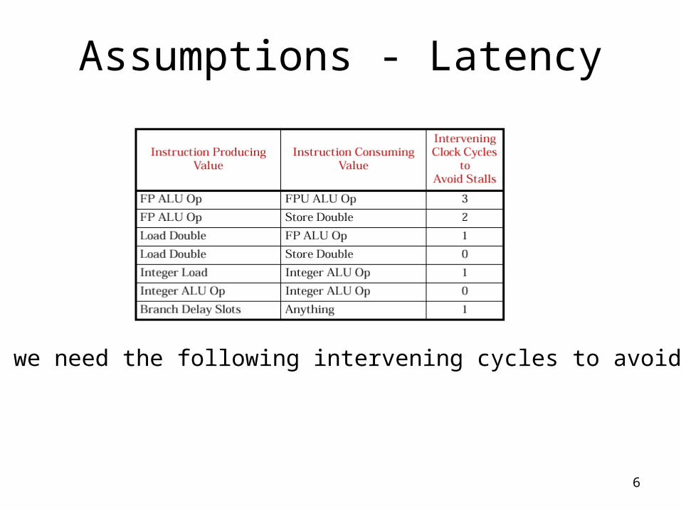
Assumptions - Latency

Assume we need the following intervening cycles to avoid stalls

7

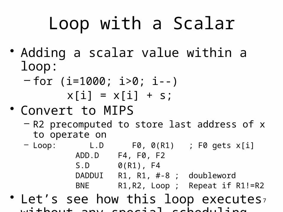
Loop with a Scalar

• Adding a scalar value within a loop:– for (i=1000; i>0; i--)

x[i] = x[i] + s;• Convert to MIPS

– R2 precomputed to store last address of x to operate on– Loop: L.D F0, 0(R1) ; F0 gets x[i]

ADD.D F4, F0, F2S.D 0(R1), F4DADDUI R1, R1, #-8 ; doublewordBNE R1,R2, Loop ; Repeat if

R1!=R2

• Let’s see how this loop executes without any special scheduling

8

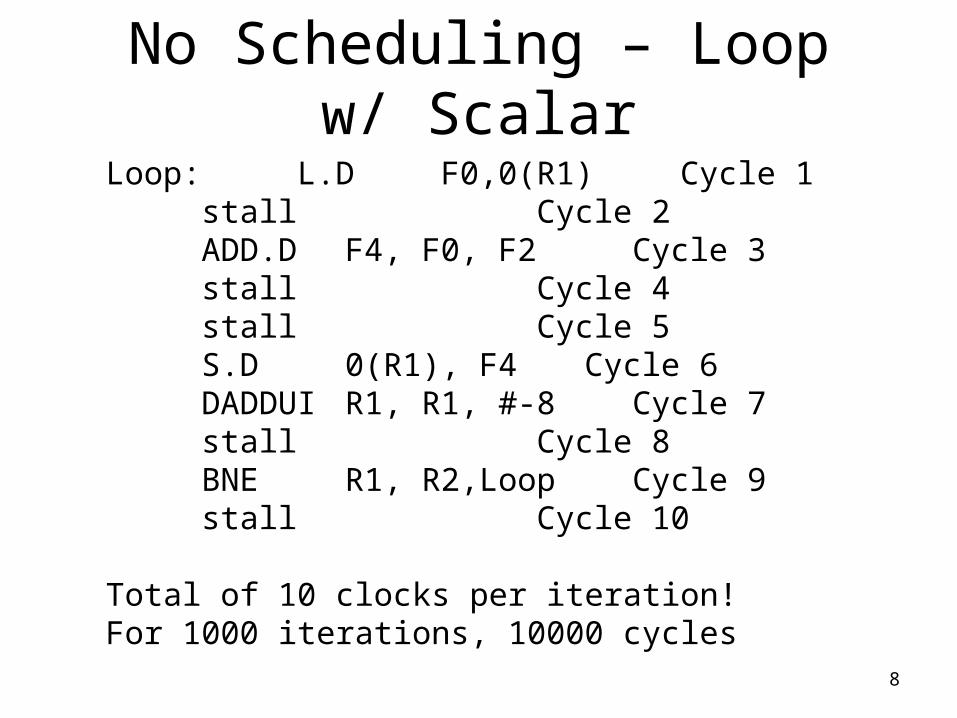
No Scheduling – Loop w/ Scalar

Loop: L.D F0,0(R1) Cycle 1stall Cycle 2ADD.D F4, F0, F2 Cycle 3stall Cycle 4stall Cycle 5S.D 0(R1), F4 Cycle 6DADDUI R1, R1, #-8 Cycle 7stall Cycle 8BNE R1, R2,Loop Cycle 9stall Cycle 10

Total of 10 clocks per iteration!For 1000 iterations, 10000 cycles

9

Optimized, Scheduled VersionOriginal: L.D F0, 0(R1) ; F0 gets x[i]

ADD.D F4, F0, F2

S.D 0(R1), F4

DADDUI R1, R1, #-8 ;doubleword

BNE R1, R2, Loop ;Repeat

Move S.D after BNE into the delay slot, move DADDUI up!

New: L.D F0, 0(R1) ; F0 gets x[i]

stall

ADD.D F4, F0, F2

DADDUI R1, R1, #-8

stall

BNE R1, R2, Loop ; Repeat

SD 8(R1), F4

Have to add 8 as SD’s offset because we already subtracted 8 off!From 10 to 7 cycles per iteration (7000 cycles total)Not a trivial computation, many compilers won’t do this

10

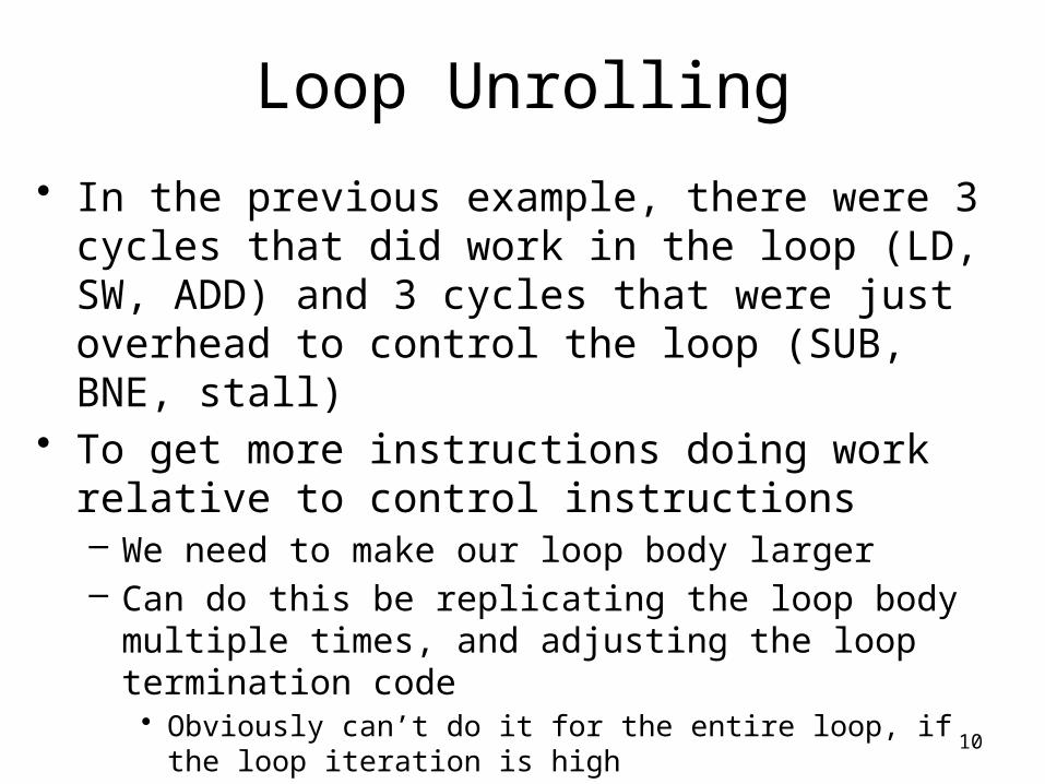
Loop Unrolling

• In the previous example, there were 3 cycles that did work in the loop (LD, SW, ADD) and 3 cycles that were just overhead to control the loop (SUB, BNE, stall)

• To get more instructions doing work relative to control instructions– We need to make our loop body larger– Can do this be replicating the loop body multiple times, and

adjusting the loop termination code• Obviously can’t do it for the entire loop, if the loop iteration is high

– Called loop unrolling• Tradeoff: Longer code, but higher ILP

11

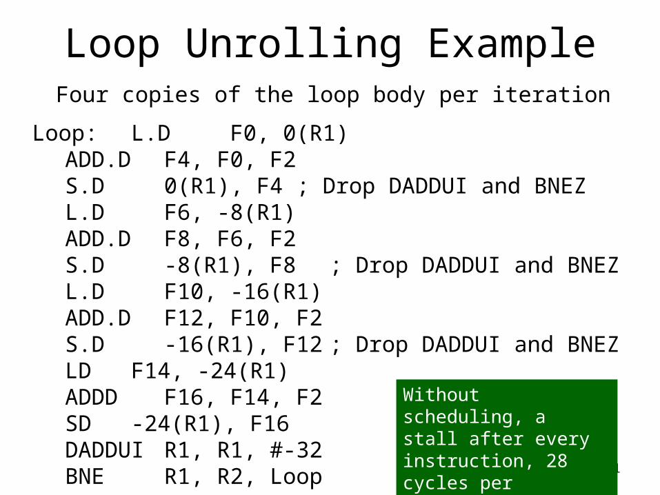
Loop Unrolling ExampleFour copies of the loop body per iteration

Loop: L.D F0, 0(R1)ADD.D F4, F0, F2S.D 0(R1), F4 ; Drop DADDUI and BNEZL.D F6, -8(R1)ADD.D F8, F6, F2S.D -8(R1), F8 ; Drop DADDUI and BNEZL.D F10, -16(R1)ADD.D F12, F10, F2S.D -16(R1), F12 ; Drop DADDUI and BNEZLD F14, -24(R1)ADDD F16, F14, F2SD -24(R1), F16DADDUI R1, R1, #-32BNE R1, R2, Loop

Without scheduling, a stall after every instruction, 28 cycles per iteration,28*250 = 7000 cycles total

12

Scheduling the Unrolled LoopLoop: L.D F0, 0(R1)

L.D F6, -8(R1)L.D F10,-16(R1)L.D F14,-24(R1)ADD.D F4, F0, F2ADD.D F8, F6, F2ADD.D F12, F10, F2ADD.D F16, F14, F2S.D 0(R1), F4S.D -8(R1), F8DADDUI R1, R1, #-32S.D 16(R1), F12BNE R1, R2, LoopS.D 8(R1), F16 ; -24=8-32

Shuffle unrolled loop instead of concatenating

No stalls! Must incorporate previous tricks of filling the delay slot

14 instructions, 14*250 = 3500 cycles total

13

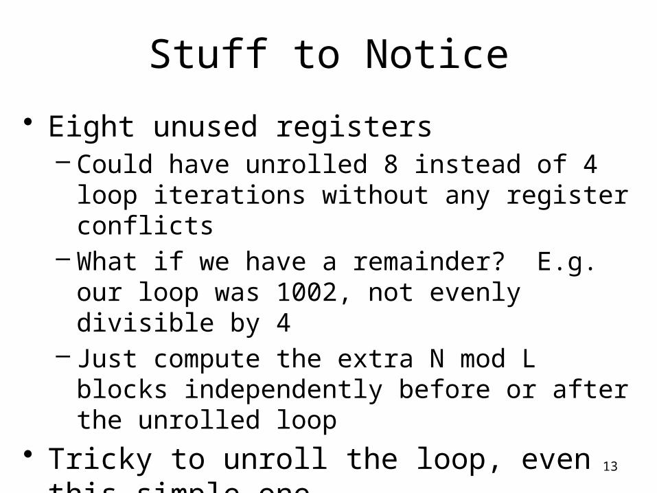
Stuff to Notice

• Eight unused registers– Could have unrolled 8 instead of 4 loop iterations

without any register conflicts– What if we have a remainder? E.g. our loop was 1002,

not evenly divisible by 4– Just compute the extra N mod L blocks independently

before or after the unrolled loop

• Tricky to unroll the loop, even this simple one– 3 types of dependence: data, name, and control

14

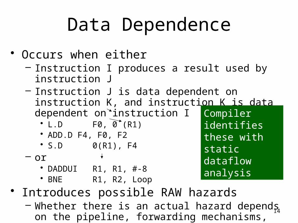
Data Dependence

• Occurs when either– Instruction I produces a result used by instruction J– Instruction J is data dependent on instruction K, and instruction

K is data dependent on instruction I• L.D F0, 0 (R1)• ADD.D F4, F0, F2• S.D 0(R1), F4

– or• DADDUI R1, R1, #-8• BNE R1, R2, Loop

• Introduces possible RAW hazards– Whether there is an actual hazard depends on the pipeline,

forwarding mechanisms, split cycle, etc.

Compiler identifies these with static dataflow analysis

15

Name Dependence• Occurs when

– 2 instructions use the same register name without a data dependence

• If I precedes J– I is antidependent on J when J writes a register that I reads

• a WAR hazard• ordering must be preserved to avoid the hazard

– I is output dependent on J if both I and J write to the same register• WAW hazard

• E.g. occurs if we unroll a loop but don’t changing the register names– This can be solved by renaming registers via the compiler, or

we can also do this dynamically

16

Name Dependence Example

Loop: L.D F0, 0(R1)

ADD.D F4, F0, F2

S.D 0(R1), F4

L.D F0, -8(R1)

ADD.D F4, F0, F2

S.D -8(R1), F4

Part of unrolled loop, always going to F0:

Name dependencies force execution stalls to avoid potential WAW or WAR problems

Eliminated by renaming the registers as in earlier example

17

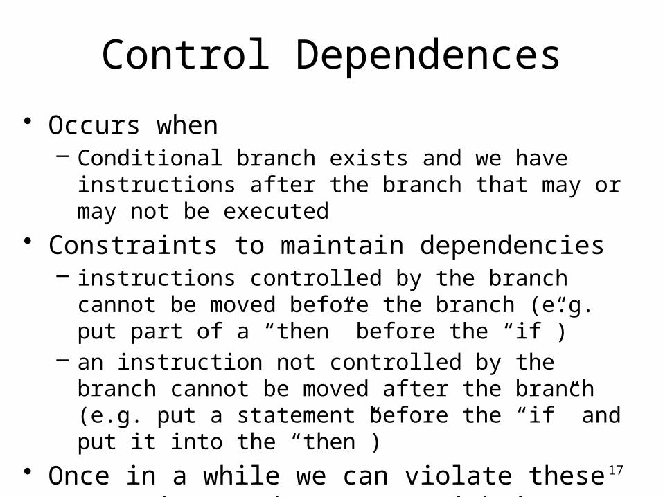
Control Dependences

• Occurs when– Conditional branch exists and we have instructions after the

branch that may or may not be executed

• Constraints to maintain dependencies– instructions controlled by the branch cannot be moved before

the branch (e.g. put part of a “then” before the “if”)– an instruction not controlled by the branch cannot be moved

after the branch (e.g. put a statement before the “if” and put it into the “then”)

• Once in a while we can violate these constraints and get away with it…

18

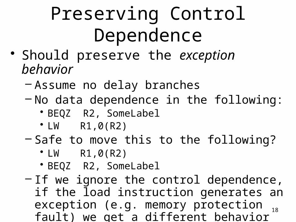
Preserving Control Dependence

• Should preserve the exception behavior– Assume no delay branches– No data dependence in the following:

• BEQZ R2, SomeLabel• LW R1,0(R2)

– Safe to move this to the following?• LW R1,0(R2)• BEQZ R2, SomeLabel

– If we ignore the control dependence, if the load instruction generates an exception (e.g. memory protection fault) we get a different behavior

19

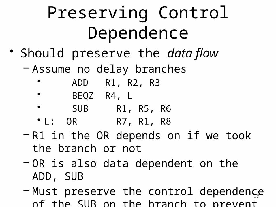
Preserving Control Dependence

• Should preserve the data flow– Assume no delay branches

• ADD R1, R2, R3• BEQZ R4, L• SUB R1, R5, R6• L: OR R7, R1, R8

– R1 in the OR depends on if we took the branch or not– OR is also data dependent on the ADD, SUB– Must preserve the control dependence of the SUB on

the branch to prevent an illegal change to the data flow

20

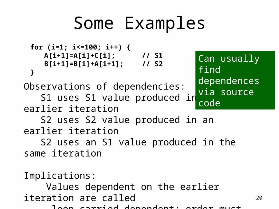
Some Examplesfor (i=1; i<=100; i++) {

A[i+1]=A[i]+C[i]; // S1B[i+1]=B[i]+A[i+1]; // S2

}

Observations of dependencies: S1 uses S1 value produced in an earlier iteration S2 uses S2 value produced in an earlier iteration S2 uses an S1 value produced in the same iteration

Implications: Values dependent on the earlier iteration are called loop carried dependent; order must be preserved non- loop carried dependences we can try and execute in parallel (but not in this case, due to other dependency)

Can usually find dependences via source code

21

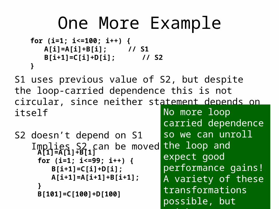
One More Examplefor (i=1; i<=100; i++) {

A[i]=A[i]+B[i]; // S1B[i+1]=C[i]+D[i]; // S2

}

S1 uses previous value of S2, but despite the loop-carried dependence this is not circular, since neither statement depends on itself

S2 doesn’t depend on S1 Implies S2 can be moved!

A[1]=A[1]+B[1]for (i=1; i<=99; i++) {

B[i+1]=C[i]+D[i];A[i+1]=A[i+1]+B[i+1];

}B[101]=C[100]+D[100]

No more loop carried dependence so we can unroll the loop and expect good performance gains!A variety of these transformations possible, but tricky

22

Instruction-Level ParallelismDynamic Branch Prediction

23

Reducing Branch Penalties

• Previously discussed – static schemes– Move branch calculation earlier in pipeline– Static branch prediction

• Always taken, not taken– Delayed branch– Loop unrolling

• Good, but limited to loops

• This section – dynamic schemes• A more general dynamic scheme that can be used with all

branches– Dynamic branch prediction

24

Dynamic Branch Prediction

• Becomes crucial to any processor that tries to issue more than one instruction per cycle– Scoreboard, Tomasulo’s algorithm we will see later operate on

a basic block (no branches)• Possible to extend Tomasulo’s algorithm to include branches

– Just not enough instructions in a basic block to get the superscalar performance

• Result– Control dependencies can become the limiting factor

• Hard for compilers to deal with, so may be ignored, resulting in a higher frequency of branches

– Amdahl’s Law too• As CPI decreases the impact of control stalls increases

25

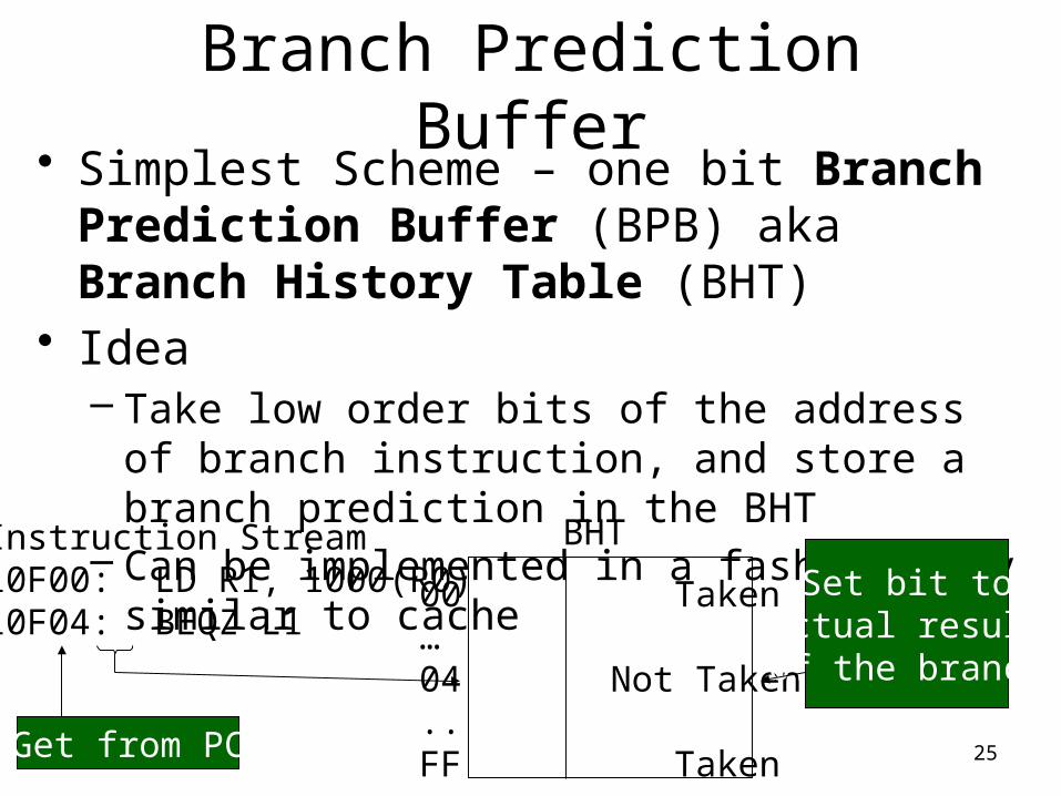
Branch Prediction Buffer• Simplest Scheme – one bit Branch Prediction

Buffer (BPB) aka Branch History Table (BHT)• Idea

– Take low order bits of the address of branch instruction, and store a branch prediction in the BHT

– Can be implemented in a fashion very similar to cache

Instruction Stream10F00: LD R1, 1000(R0)10F04: BEQZ L1

BHT

00 Taken…04 Not Taken..FF TakenGet from PC

Set bit toactual resultof the branch

26

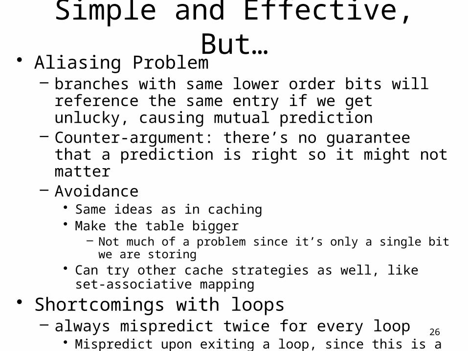
Simple and Effective, But…• Aliasing Problem

– branches with same lower order bits will reference the same entry if we get unlucky, causing mutual prediction

– Counter-argument: there’s no guarantee that a prediction is right so it might not matter

– Avoidance• Same ideas as in caching• Make the table bigger

– Not much of a problem since it’s only a single bit we are storing• Can try other cache strategies as well, like set-associative mapping

• Shortcomings with loops– always mispredict twice for every loop

• Mispredict upon exiting a loop, since this is a surprise• If we repeat the loop, we’ll miss again since we’ll predict to not take the

branch• Book example: branch taken 90% of time predicted 80% accuracy

27

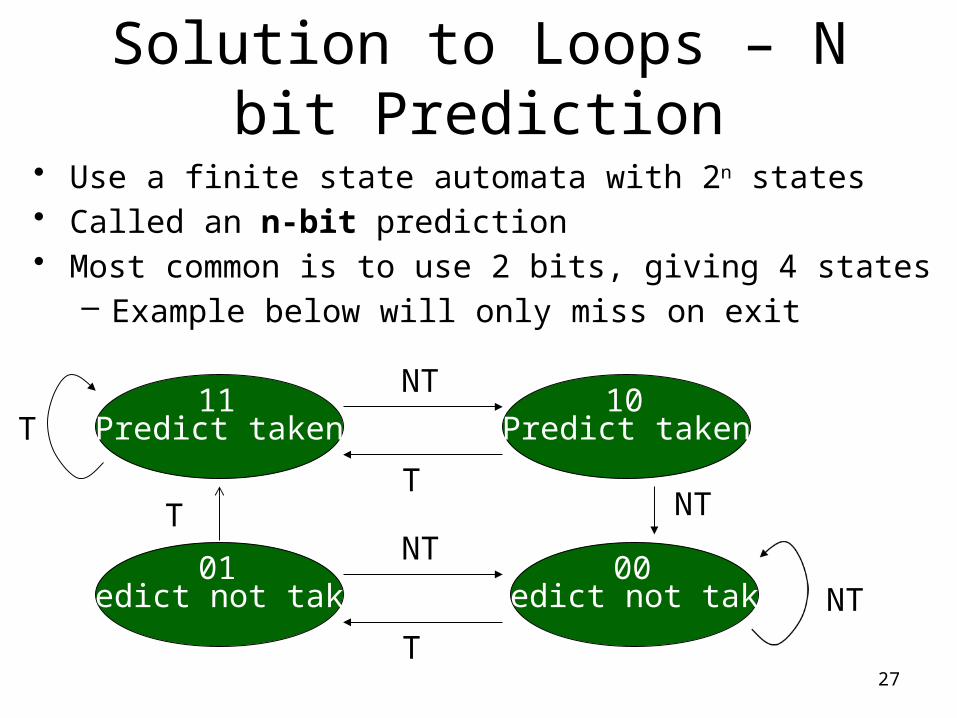
Solution to Loops – N bit Prediction

• Use a finite state automata with 2n states• Called an n-bit prediction• Most common is to use 2 bits, giving 4 states

– Example below will only miss on exit

Predict taken Predict taken

Predict not taken Predict not taken

11

01

10

00

T

NT

T

NT

T

T NT

NT

28

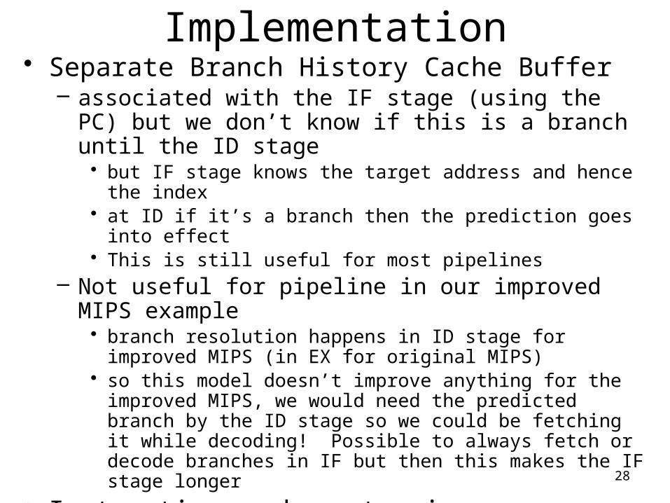
Implementation• Separate Branch History Cache Buffer

– associated with the IF stage (using the PC) but we don’t know if this is a branch until the ID stage• but IF stage knows the target address and hence the index• at ID if it’s a branch then the prediction goes into effect• This is still useful for most pipelines

– Not useful for pipeline in our improved MIPS example• branch resolution happens in ID stage for improved MIPS (in EX for

original MIPS)• so this model doesn’t improve anything for the improved MIPS, we

would need the predicted branch by the ID stage so we could be fetching it while decoding! Possible to always fetch or decode branches in IF but then this makes the IF stage longer

• Instruction cache extension– hold the bits with the instruction in the Instruction Cache as an early branch

indicator – Increased cost since the bits will take up space for non- branch instructions

as well

29

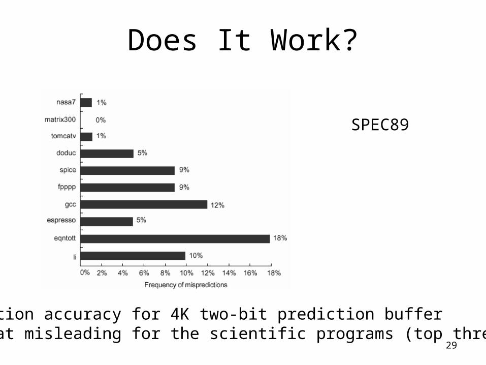
Does It Work?

SPEC89

Prediction accuracy for 4K two-bit prediction bufferSomewhat misleading for the scientific programs (top three)

30

Increased Table SizeIncreasing the table size helps with caching, does it help here?

We can simulate branch prediction quite easily. The answer is NO compared to an unlimited size table!

Performance bottleneck is the actual goodness of our prediction algorithm

31

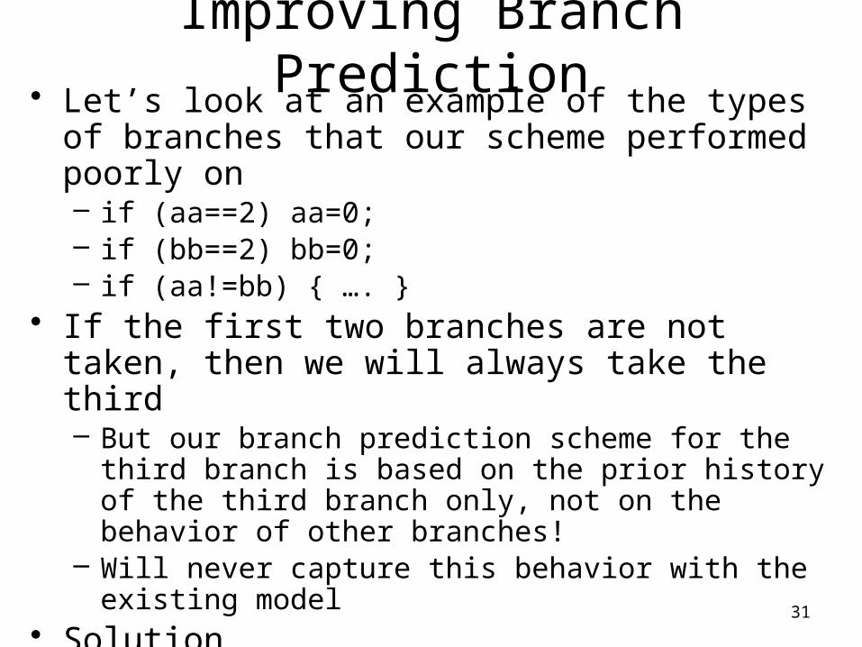
Improving Branch Prediction• Let’s look at an example of the types of branches that our

scheme performed poorly on– if (aa==2) aa=0;– if (bb==2) bb=0;– if (aa!=bb) { …. }

• If the first two branches are not taken, then we will always take the third– But our branch prediction scheme for the third branch is based

on the prior history of the third branch only, not on the behavior of other branches!

– Will never capture this behavior with the existing model• Solution

– Use a correlating predictor, or what happened on the previous (in a dynamic sense, not static sense) branch

– Not necessarily a good predictor (consider spaghetti code)

32

Example – Correlating Predictor

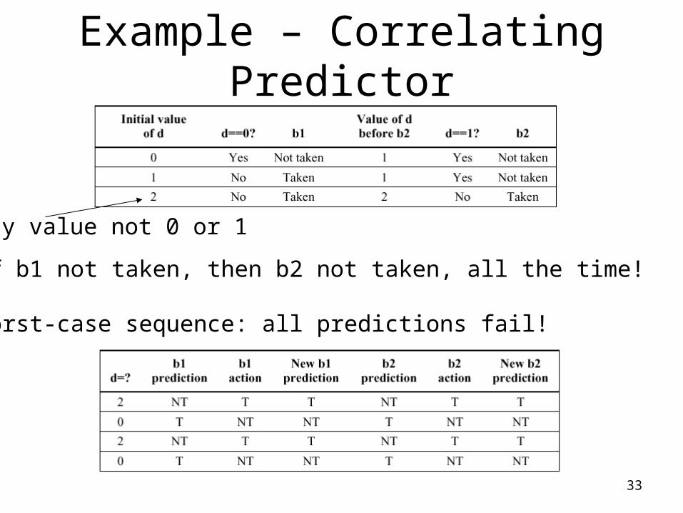
• Consider the following code fragment– if (d==0) d=1;– if (d==1) { … }

• Typical code generated by this fragment– BNEZ R1, L1 ; check if d==0 B1– ADDI R1, R0, #1 ; d1– L1: SEQI R3, R1, #1 ; Set R3 if R1==1– BNEZ R3, L2 ; Skip if d!=1 B2– L2: …

• Let’s look at all the possible outcomes based on the value of d going into this code

33

Example – Correlating Predictor

Any value not 0 or 1

If b1 not taken, then b2 not taken, all the time!

Worst-case sequence: all predictions fail!

34

Solution – Use correlator

• Use a predictor with one bit of correlation– i.e. we remember what happened with the last branch to predict the current

branch– Think of this as the last branch has two separate prediction bits

• One bit assuming the last branch was taken• One bit assuming the last branch was not taken

• Pair the prediction bits: first bit is the prediction if the last branch is not taken, second bit is the prediction if the last branch is taken

• Leads to 4 possibilities: which way the last one went chooses the prediction– (Last-taken, last-not-taken) X (predict-taken, predict-not-taken)

35

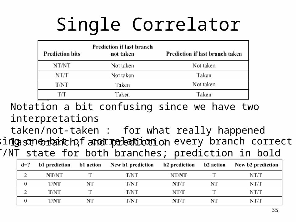
Single Correlator

Notation a bit confusing since we have two interpretationstaken/not-taken : for what really happened last branch, and prediction

Behavior using one-bit of correlation : every branch correct except firstStart in NT/NT state for both branches; prediction in bold

36

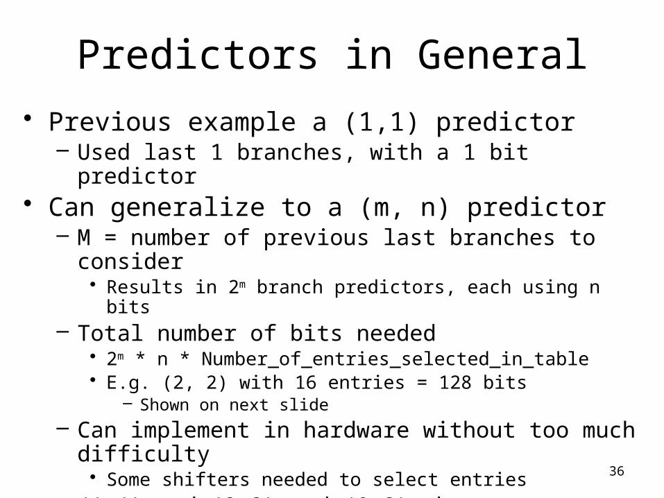
Predictors in General

• Previous example a (1,1) predictor– Used last 1 branches, with a 1 bit predictor

• Can generalize to a (m, n) predictor– M = number of previous last branches to consider

• Results in 2m branch predictors, each using n bits– Total number of bits needed

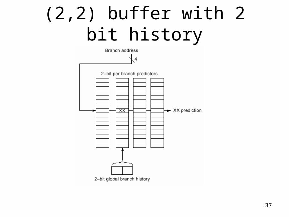
• 2m * n * Number_of_entries_selected_in_table• E.g. (2, 2) with 16 entries = 128 bits

– Shown on next slide

– Can implement in hardware without too much difficulty• Some shifters needed to select entries

– (1,1) and (2,2) and (0,2) the most interesting/common selections

37

(2,2) buffer with 2 bit history

38

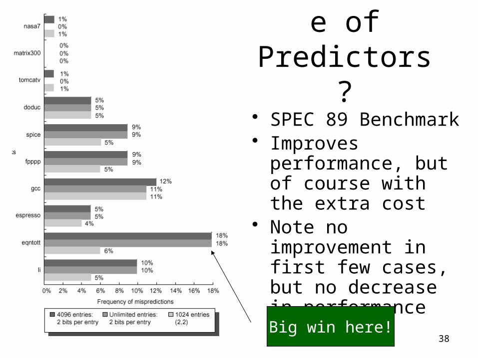
Performance of Predictors?

• SPEC 89 Benchmark• Improves performance,

but of course with the extra cost

• Note no improvement in first few cases, but no decrease in performance either

Big win here!

39

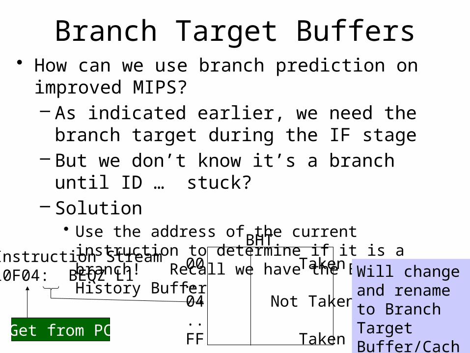
Branch Target Buffers• How can we use branch prediction on improved MIPS?

– As indicated earlier, we need the branch target during the IF stage

– But we don’t know it’s a branch until ID … stuck?– Solution

• Use the address of the current instruction to determine if it is a branch! Recall we have the Branch History Buffer

00 Taken…04 Not Taken..FF TakenGet from PC

Instruction Stream10F04: BEQZ L1

BHT

Will change and rename to Branch Target Buffer/Cache

40

Branch Target Buffer

• Need to change a bit from Branch History Table– Store the actual Predicted PC with the branch prediction for

each entry– If an entry exists in the BTB, this lets us look up the Predicted

PC during the IF stage, and then use this Predicted PC for the IF of the next instruction during the ID of the branch instruction

41

BTB Diagram

42

Steps in our MIPS

Arch

This really meanscorrect prediction

43

Penalties

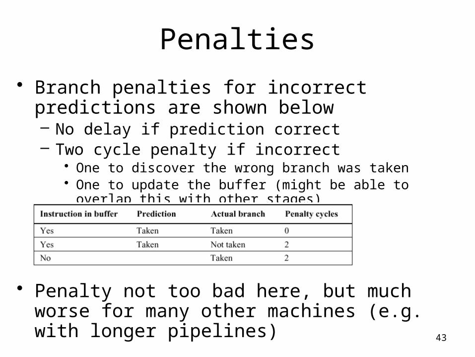
• Branch penalties for incorrect predictions are shown below– No delay if prediction correct– Two cycle penalty if incorrect

• One to discover the wrong branch was taken• One to update the buffer (might be able to overlap this with other stages)

• Penalty not too bad here, but much worse for many other machines (e.g. with longer pipelines)

44

Other Improvements• Branch Folding

– Store the target instruction in the cache, not the address– We can then start executing this instruction directly instead of having to

fetch it! • Branch “disappears” for unconditional branches• Will then update the PC during the EX stage• Used with some VLIW architectures (e.g. CRISP)• Increases buffer size, but removes an IF stage• Complicates hardware

• Predict Indirect Jumps– Dynamic Jumps, target changes– Used most frequently for Returns – Implies a stack, so we could try a stack-based prediction scheme, caching

the recent return addresses– Can combine with folding to get Indirect Jump Folding

• Predication– Do the If and Else at the same time, select correct one later

45

Branch Prediction Summary

• Active Research Topic – Tons of papers and ideas coming out on branch prediction

• Easy to simulate• Easy to forget about costs

– Motivation is real though• Mispredicted branches are a large bottleneck and a small percent

improvement in prediction can lead to larger overall speedup• Intel has claimed that up to 30% of processor performance gets tossed

out the window because of those 5-10% wrong branches

• Basic concepts presented here used in one form or another in most systems today

46

Example – Intel Pentium Branch Prediction

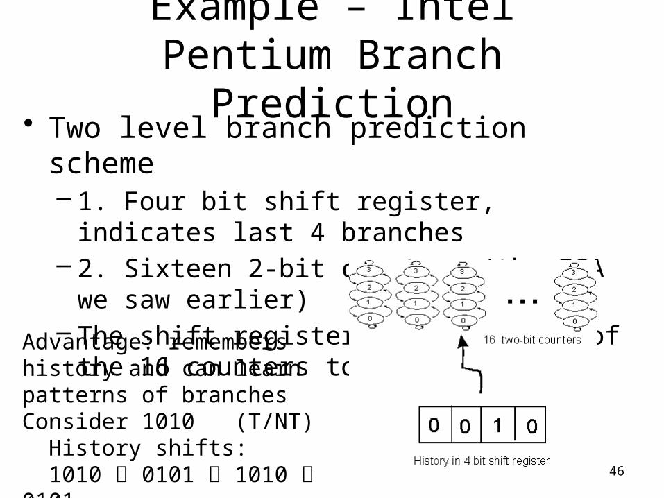
• Two level branch prediction scheme– 1. Four bit shift register, indicates last 4 branches– 2. Sixteen 2-bit counters (the FSA we saw earlier)– The shift register selects which of the 16 counters to

use

Advantage: remembers history and can learn patterns of branchesConsider 1010 (T/NT) History shifts: 1010 0101 1010 0101Update 5th and 10th counters

47

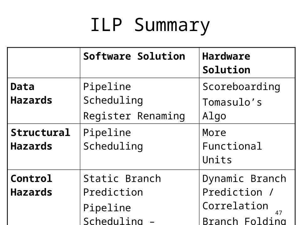
ILP Summary

Software Solution Hardware Solution

Data Hazards Pipeline SchedulingRegister Renaming

ScoreboardingTomasulo’s Algo

Structural Hazards

Pipeline Scheduling More Functional Units

Control Hazards

Static Branch Prediction Pipeline Scheduling – Delayed BranchLoop Unrolling

Dynamic Branch Prediction / CorrelationBranch FoldingPredication