DZmix v. 1.1.2

K.E. Sundell

J.E. SaylorDepartment of Earth and Atmospheric Sciences

University of Houston

Houston, TX

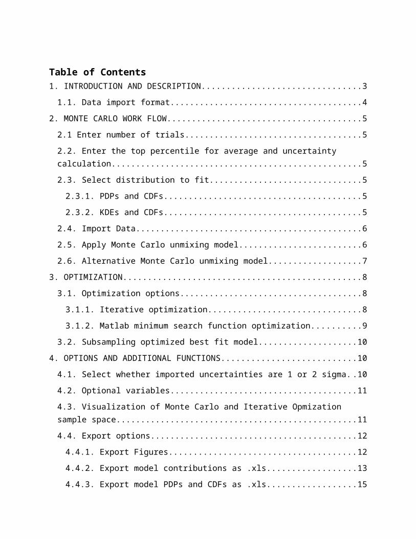
Table of Contents1. INTRODUCTION AND DESCRIPTION..................................................................................3

1.1. Data import format...............................................................................................................4

2. MONTE CARLO WORK FLOW...............................................................................................5

2.1 Enter number of trials............................................................................................................5

2.2. Enter the top percentile for average and uncertainty calculation..........................................5

2.3. Select distribution to fit........................................................................................................5

2.3.1. PDPs and CDFs.............................................................................................................5

2.3.2. KDEs and CDFs............................................................................................................5

2.4. Import Data...........................................................................................................................6

2.5. Apply Monte Carlo unmixing model....................................................................................6

2.6. Alternative Monte Carlo unmixing model............................................................................7

3. OPTIMIZATION.........................................................................................................................8

3.1. Optimization options............................................................................................................8

3.1.1. Iterative optimization.....................................................................................................8

3.1.2. Matlab minimum search function optimization.............................................................9

3.2. Subsampling optimized best fit model...............................................................................10

4. OPTIONS AND ADDITIONAL FUNCTIONS.......................................................................10

4.1. Select whether imported uncertainties are 1 or 2 sigma.....................................................10

4.2. Optional variables...............................................................................................................11

4.3. Visualization of Monte Carlo and Iterative Opmization sample space..............................11

4.4. Export options.....................................................................................................................12

4.4.1. Export Figures.............................................................................................................12

4.4.2. Export model contributions as .xls..............................................................................13

4.4.3. Export model PDPs and CDFs as .xls.........................................................................15

4.4.4. Plot Relative Contributions..........................................................................................16

1. INTRODUCTION AND DESCRIPTIONDZmix is designed to calculate quantitative mixing models for detrital geochronology

data. Random mixtures of potential source samples are compared to a target by calculating the Cross-correlation coefficient, Kuiper test V value, and Kolmogorov-Smirnov test D value. Mixtures which are the most similar to the target based on these metrics are retained, providing an average and uncertainties for the best fit models. Additionally, the results of the Monte Carlo mixture modeling can be used as an initial guess for an optimized step which yields the single best fit between model and target. The workflow is organized sequentially so that users can easily produce results (Fig. 2).

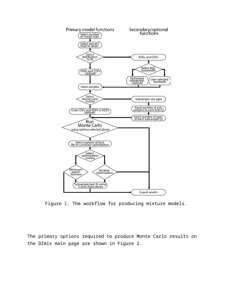
Figure 1. The workflow for producing mixture models.

The primary options required to produce Monte Carlo results on the DZmix main page are shown in Figure 2.

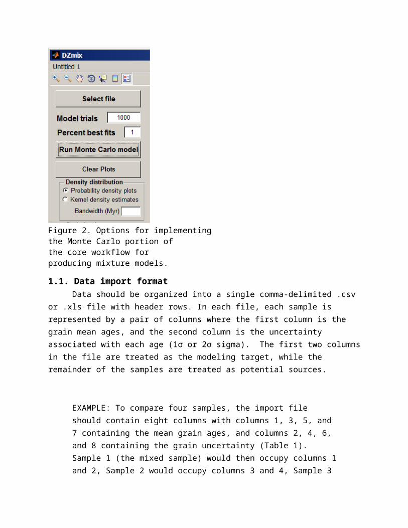
Figure 2. Options for implementingthe Monte Carlo portion of the core workflow for producing mixture models.

1.1. Data import formatData should be organized into a single comma-delimited .csv or .xls file with header

rows. In each file, each sample is represented by a pair of columns where the first column is the grain mean ages, and the second column is the uncertainty associated with each age (1σ or 2σ sigma). The first two columns in the file are treated as the modeling target, while the remainder of the samples are treated as potential sources.

EXAMPLE: To compare four samples, the import file should contain eight columns with columns 1, 3, 5, and 7 containing the mean grain ages, and columns 2, 4, 6, and 8 containing the grain uncertainty (Table 1). Sample 1 (the mixed sample) would then occupy columns 1 and 2, Sample 2 would occupy columns 3

and 4, Sample 3 would occupy columns 5 and 6, and Sample 4 would occupy columns 7 and 8.

NOTE: If any ages in the input file are exactly the same, the code will crash. Avoid this by adding some insignificant amount (e.g., 10-6) to identical ages prior to data import.

Table 1. Example of the first three rows of an input file. Mixed sample name

2sigma Uncertainty

Source 1 name

2sigma Uncertainty

Source 2 name

2sigma Uncertainty

Source 3 name

2sigma Uncertainty

72.3 17.8 45.7 1.2 259.6 13.2 255.6 19.8

75.9 21.8 45.9 1.4 264.5 7.6 257.8 4.2

2. MONTE CARLO WORK FLOW

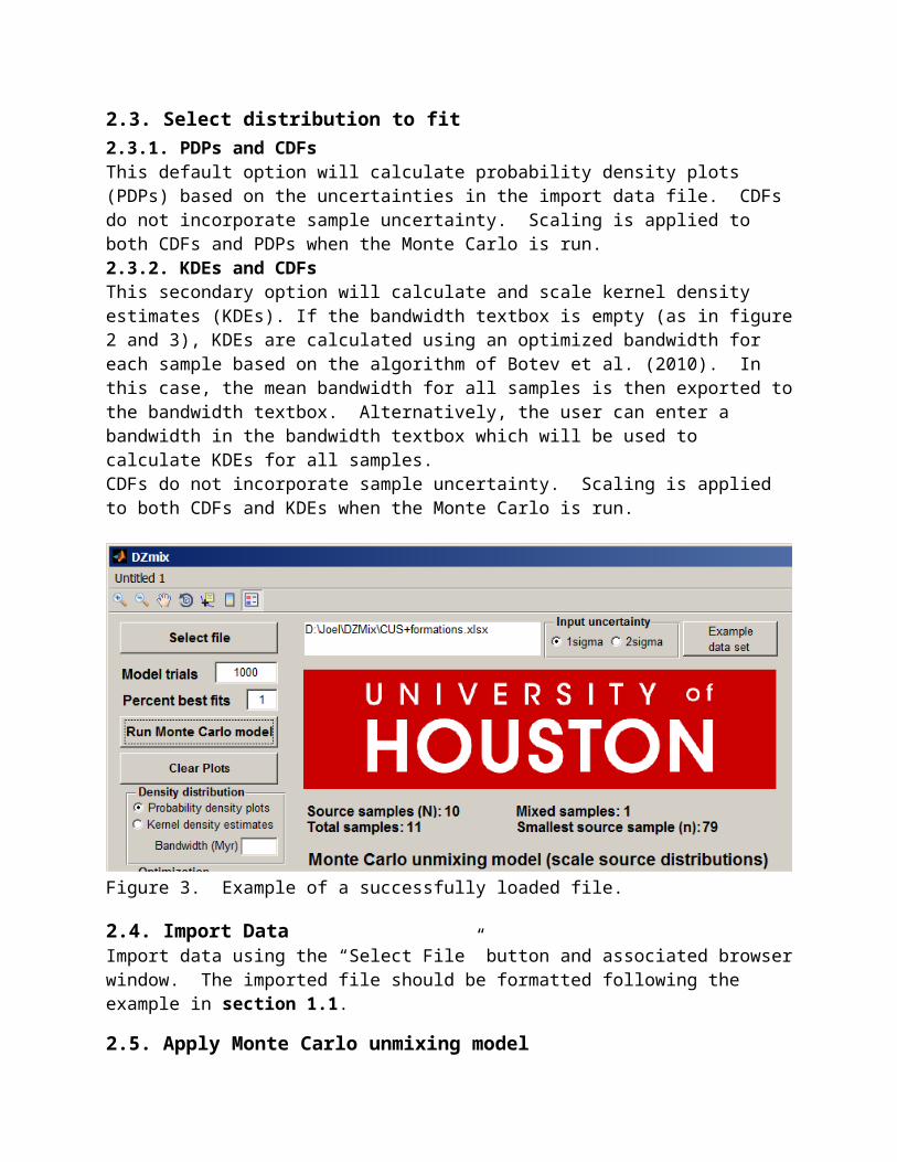
2.1 Enter number of trials. This sets the number of random mixtures of source samples that are produced. The code will run until this number of models is produced. Select File. Use the “Browser” button to browse for, and import, the data (Figure 2). When the file is successfully loaded, the file path will be displayed below the University of Houston logo and the bold text below will update to indicate how many samples have been loaded.

2.2. Enter the top percentile for average and uncertainty calculationEnter top percentile. This sets the top percentile (of the number of trials entered in step 2.1.) which will be retained and used to calculate average source contributions and their associated standard deviations.

2.3. Select distribution to fit2.3.1. PDPs and CDFsThis default option will calculate probability density plots (PDPs) based on the uncertainties in the import data file. CDFs do not incorporate sample uncertainty. Scaling is applied to both CDFs and PDPs when the Monte Carlo is run. 2.3.2. KDEs and CDFsThis secondary option will calculate and scale kernel density estimates (KDEs). If the bandwidth textbox is empty (as in figure 2 and 3), KDEs are calculated using an optimized bandwidth for each sample based on the algorithm of Botev et al. (2010). In this case, the mean bandwidth for all samples is then exported to the bandwidth textbox. Alternatively, the user can enter a bandwidth in the bandwidth textbox which will be used to calculate KDEs for all samples.

CDFs do not incorporate sample uncertainty. Scaling is applied to both CDFs and KDEs when the Monte Carlo is run.

Figure 3. Example of a successfully loaded file.

2.4. Import DataImport data using the “Select File” button and associated browser window. The imported file should be formatted following the example in section 1.1.

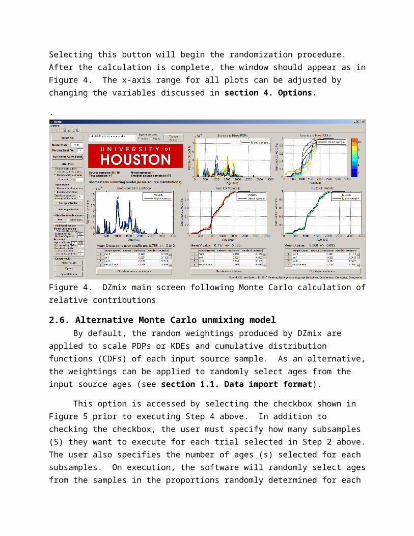
2.5. Apply Monte Carlo unmixing modelSelecting this button will begin the randomization procedure. After the calculation is complete, the window should appear as in Figure 4. The x-axis range for all plots can be adjusted by changing the variables discussed in section 4. Options.

.

Figure 4. DZmix main screen following Monte Carlo calculation of relative contributions

2.6. Alternative Monte Carlo unmixing modelBy default, the random weightings produced by DZmix are applied to scale PDPs or

KDEs and cumulative distribution functions (CDFs) of each input source sample. As an alternative, the weightings can be applied to randomly select ages from the input source ages (see section 1.1. Data import format).

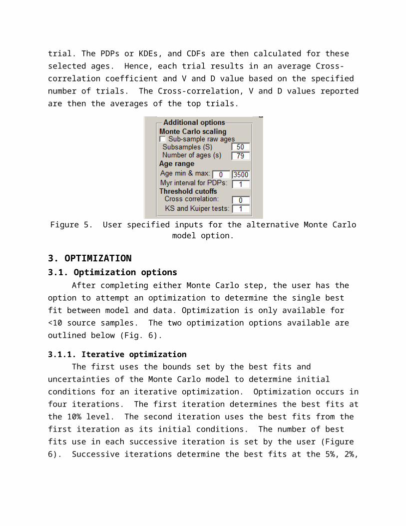
This option is accessed by selecting the checkbox shown in Figure 5 prior to executing Step 4 above. In addition to checking the checkbox, the user must specify how many subsamples (S) they want to execute for each trial selected in Step 2 above. The user also specifies the number of ages (s) selected for each subsamples. On execution, the software will randomly select ages from the samples in the proportions randomly determined for each trial. The PDPs or KDEs, and CDFs are then calculated for these selected ages. Hence, each trial results in an average Cross-correlation coefficient and V and D value based on the specified number of trials. The Cross-correlation, V and D values reported are then the averages of the top trials.

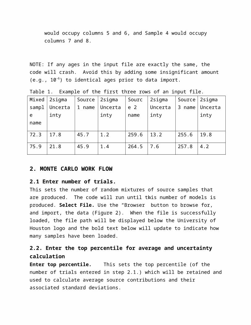
Figure 5. User specified inputs for the alternative Monte Carlo model option.

3. OPTIMIZATION3.1. Optimization options

After completing either Monte Carlo step, the user has the option to attempt an optimization to determine the single best fit between model and data. Optimization is only available for <10 source samples. The two optimization options available are outlined below (Fig. 6).

3.1.1. Iterative optimizationThe first uses the bounds set by the best fits and uncertainties of the Monte Carlo model

to determine initial conditions for an iterative optimization. Optimization occurs in four iterations. The first iteration determines the best fits at the 10% level. The second iteration uses the best fits from the first iteration as its initial conditions. The number of best fits use in each successive iteration is set by the user (Figure 6). Successive iterations determine the best fits at the 5%, 2%, and 1% levels. The output of a successful Iterative Optimization is shown in Figure 6.

Figure 6. Options for model optimization.

3.1.2. Matlab minimum search function optimizationThe alternative approach executes the minimum search function included in the Matlab

Optimization Toolbox. The user specified (Figure 3) best fits from the Monte Carlo model are used as initial conditions after which the model searchs for a global minimum in D or V values or maximum in Cross-correlation coefficient.

Figure 7. Results of a successful Iterative Optimization.

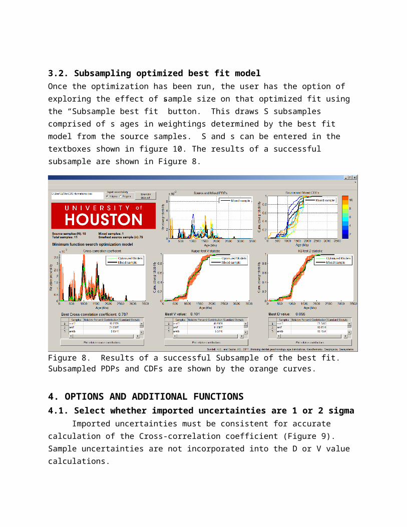
3.2. Subsampling optimized best fit modelOnce the optimization has been run, the user has the option of exploring the effect of sample size on that optimized fit using the “Subsample best fit” button. This draws S subsamples comprised of s ages in weightings determined by the best fit model from the source samples. S and s can be entered in the textboxes shown in figure 10. The results of a successful subsample are shown in Figure 8.

Figure 8. Results of a successful Subsample of the best fit. Subsampled PDPs and CDFs are shown by the orange curves.

4. OPTIONS AND ADDITIONAL FUNCTIONS4.1. Select whether imported uncertainties are 1 or 2 sigma

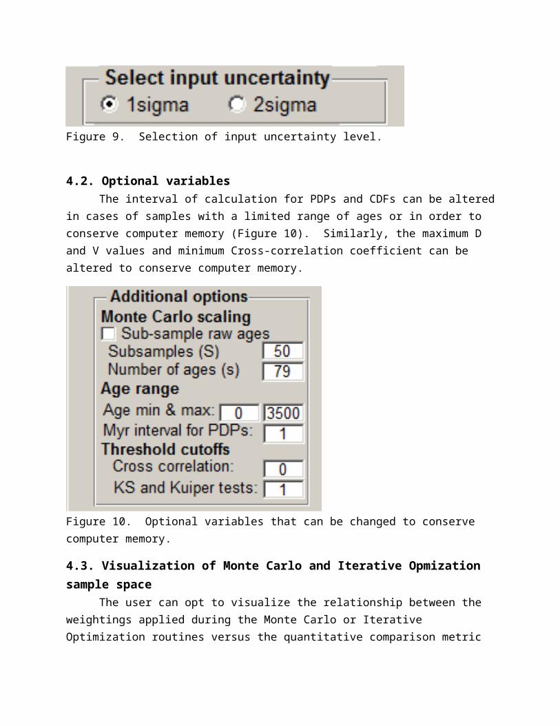
Imported uncertainties must be consistent for accurate calculation of the Cross-correlation coefficient (Figure 9). Sample uncertainties are not incorporated into the D or V value calculations.

Figure 9. Selection of input uncertainty level.

4.2. Optional variablesThe interval of calculation for PDPs and CDFs can be altered in cases of samples with a

limited range of ages or in order to conserve computer memory (Figure 10). Similarly, the maximum D and V values and minimum Cross-correlation coefficient can be altered to conserve computer memory.

Figure 10. Optional variables that can be changed to conserve computer memory.

4.3. Visualization of Monte Carlo and Iterative Opmization sample spaceThe user can opt to visualize the relationship between the weightings applied during the

Monte Carlo or Iterative Optimization routines versus the quantitative comparison metric (D or V values or Cross-correlation coefficient) that they produced using the “Visualize model search space” option;. This option can be extremely time and compute-intensive. The results of two runs are shown in Figure 11.

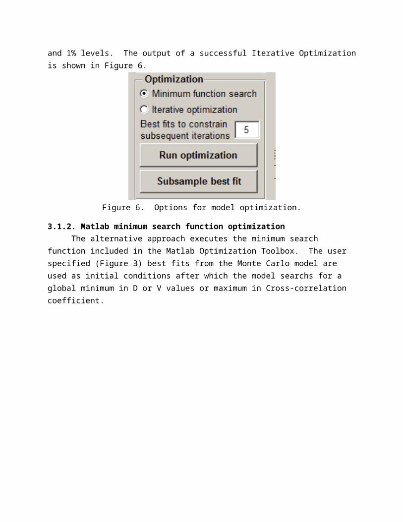
Figure 11. Results of a visualization of the Monte Carlo (left) and Iterative Optimization (right) search space.

4.4. Export options4.4.1. Export FiguresThe “Export Figures” button will export the three graphs shown in Figures 12 and 13 as individual figures for saving. Figure 14 shows one of the figures exported using the “Export Figures” button.

Figure 12. Probability density plots and cumulative distribution functions of the input potential sources and target. Note that the first samples in the input file is the target and subsequent sources are numbered 1–N and colored according to the colorbar on the right.

Figure 13. Probability density plots and cumulative distribution functions for the input target and the top percentile of model runs selected in step 2.5. Also shown are the Cross-correlation, V and D values for the single model that best matches the target.

Figure 14. Target and model PDPs exported using the “Export Figures” button.

4.4.2. Export model contributions as .xlsThe “Export model contributions as .xls” button will export the three tables shown in Figure 8 as a single concatenated Excel spreadsheet. See Table 2 for an example of the spreadsheet created using this function. Table 2. Example of spreadsheet exported as Excel (.xls) file using the “Export model contributions as .xls” buttonResults of Matlab Optimization unmixing model

weightings applied to PDPs and CDFs

runs= 1000

percent accepted trials= 2.5

Cross-correlation cutoff= 0.5

Kuiper V value cutoff= 0.5

KS D value cutoff= 0.5

Cross-correlation

SamplesRelative Contribution Std Dev

Sample 2 Name 0.063359992 0.044883

Sample 3 Name 0.073767314 0.051989

Sample 4 Name 0.085238909 0.078571

Sample 5 Name 0.164682857 0.115984

Sample 6 Name 0.182228663 0.106802

Sample 7 Name 0.430722266 0.075628

Kuiper D value

SamplesRelative Contribution Std Dev

Sample 2 Name 0.294399024 0.082711

Sample 3 Name 0.071976221 0.046118

Sample 4 Name 0.154275195 0.146542

Sample 5 Name 0.204373487 0.116638

Sample 6 Name 0.115698835 0.086747

Sample 7 Name 0.159277238 0.133872

KS V value

Samples Relative Std Dev

Contribution

Sample 2 Name 0.063907044 0.064105

Sample 3 Name 0.071848919 0.054834

Sample 4 Name 0.147545097 0.08992

Sample 5 Name 0.203997301 0.102424

Sample 6 Name 0.119321983 0.09833

Sample 7 Name 0.393379657 0.100718

4.4.3. Export model PDPs and CDFs as .xlsThis button exports the model PDPs and CDFs shown in Figure 12 as three Excel spreadsheets.

4.4.4. Plot Relative ContributionsThe “Plot Relative Contributions” buttons adjacent to each table plots the calculated relative contribution versus the sample number as a separate figure outside of the DZmix main window (Figure 15). This is the same data that is shown in the tables in the main DZmix window.

Figure 15. Figure produced by the “Plot Relative Contributions” button. This shows the mean relative contribution of each potential source sample for the top percentile indicated in step 4 and their associated standard deviations.

Works Cited

BOTEV, Z.I., GROTOWSKI, J.F. & KROESE, D.P. (2010) Kernel Density Esitmation Via Diffusion. Annals of Statistics, 38, 2916-2957.