1 introduction - donald l. snyderdls-website.com/.../compoundanglejoinery.pdf · compound-angle...

Created: 11 August 2014 Last Revision: 4 December 2015

1

Compound-Angle JoineryDonald L. SnyderBill Gottesman1

1 Introduction

In a previous note, one of us (DLS) wrote about compound-angle joinery and stat-ed, without explanation, the mathematical expressions which specify the blade tiltand miter-gauge setup angles on a table saw used to cut the parts of a compound-angle joint [1]. The same expressions apply for other tools used to cut the joints,such as miter saws, scroll saws, and even hand saws. For completeness, the math-ematical basis for the expressions is developed in this note. In addition, the earlierFrink computer-procedure [1] for calculating the setup angles is updated to includecorrect formulas for setup angles and for not just compound miter-joints but alsocompound butt-joints, and the visual display of results on portable devices such assmart phones and tablets is improved. The mathematical basis for compound-anglejoinery is developed in two ways. For the first, in Section 3, plane trigonometry,vector notation and rotation matrices are used. For the second, in Section 4,spherical trigonometry is used following insights of Bill Gottesman.

In Section 1.1 we give some examples of objects made using compound-angle joinery. Several angles that occur in the joinery are identified in Section 2.The development of the setup angles by using plane trigonometry, vectors and ro-tation matrices is in Section 3. The development using spherical trigonometry is inSection 4. Results are summarized in Section 5, and computer implementationsare in Section 6. Section 7 has four examples, and 8 lists cited references.

1.1 Examplesofobjectsexhibitingcompound-anglejoinery

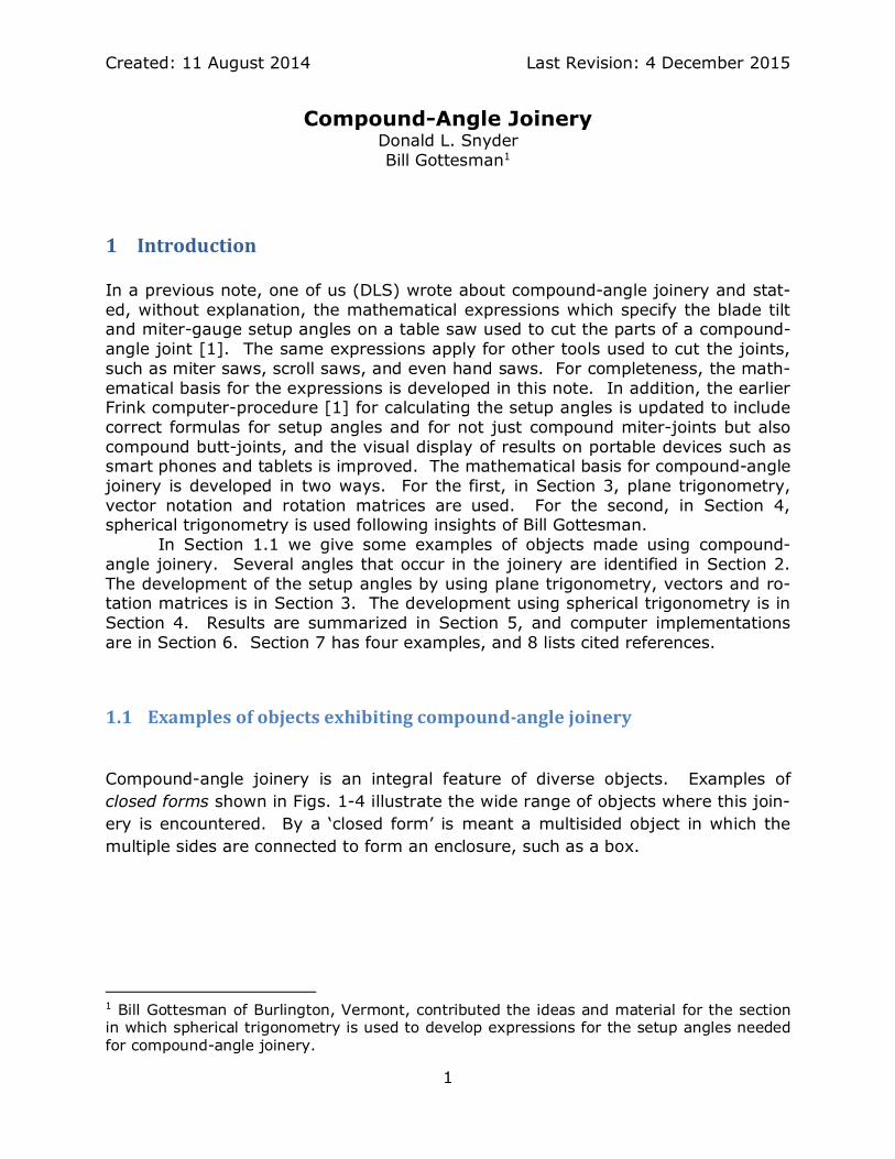
Compound-angle joinery is an integral feature of diverse objects. Examples ofclosed forms shown in Figs. 1-4 illustrate the wide range of objects where this join-ery is encountered. By a ‘closed form’ is meant a multisided object in which themultiple sides are connected to form an enclosure, such as a box.

1 Bill Gottesman of Burlington, Vermont, contributed the ideas and material for the sectionin which spherical trigonometry is used to develop expressions for the setup angles neededfor compound-angle joinery.


2

Figure 1. Octagonal jewelry box with removable shelfinsert. Made by Vic Barr using maple and cherrywoods. The eight sides are at 90° to the base.

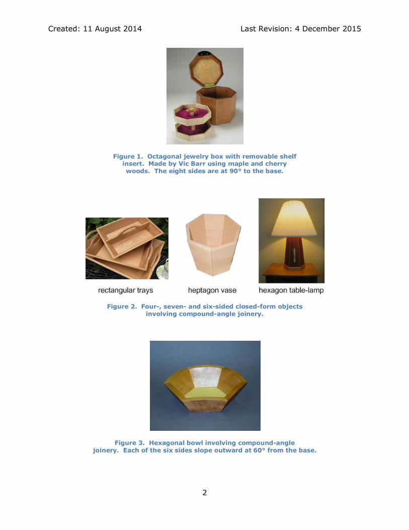
Figure 2. Four-, seven- and six-sided closed-form objectsinvolving compound-angle joinery.

Figure 3. Hexagonal bowl involving compound-anglejoinery. Each of the six sides slope outward at 60° from the base.


3

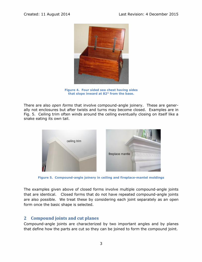
Figure 4. Four sided sea chest having sidesthat slope inward at 82° from the base.

There are also open forms that involve compound-angle joinery. These are gener-ally not enclosures but after twists and turns may become closed. Examples are inFig. 5. Ceiling trim often winds around the ceiling eventually closing on itself like asnake eating its own tail.

Figure 5. Compound-angle joinery in ceiling and fireplace-mantel moldings

The examples given above of closed forms involve multiple compound-angle jointsthat are identical. Closed forms that do not have repeated compound-angle jointsare also possible. We treat these by considering each joint separately as an openform once the basic shape is selected.

2 CompoundjointsandcutplanesCompound-angle joints are characterized by two important angles and by planesthat define how the parts are cut so they can be joined to form the compound joint.


4

2.1 Anglesthatcharacterizeacompound-anglejointsIllustrated in Fig. 6 are two components of a closed or open form that come togeth-er in a compound-angle joint. Both components are assumed to rest on the XY-plane of a three-dimensional coordinate system2, with the resting edge of one com-ponent (component 1) aligned with Y-axis and having a slope of S degrees meas-ured (counterclockwise) from the XY-plane. The origin of the coordinate system islocated at the point in the XY-plane where the two components come together. Theresting edges of the two components meet an angle π in the XY-plane. For aclosed form having the shape of an N-sided regular polygon in the XY-plane,

∋ (2 *180 /N Nπ < , ν degrees. For example, a four-sided square box will have

2 *180 / 4 90π < <ν ν regardless of any slope the sides may have, the six-sided bowlof Fig. 3 has a hexagonally shaped base with 4 *180 / 6 120π < <ν ν , and the seven-sided heptagon-vase of Fig. 2 has 5 *180 / 7 128.6π < ≡ν ν . Generally, 0 180π′ ′ ν .

There is another angle that is important in describing the joined componentsof Fig. 6. It is called the “dihedral angle.” The dihedral angle can be measured byconstructing two lines, one in the face of each component. The line in a face isconstructed so that it is perpendicular to the mating line where the two faces join.The two constructed lines are positioned to meet at common point anywhere alongthe mating line. The smallest angle between the two lines constructed in this way isthe dihedral angle (also called the plane angle [11]).

Figure 6. Compound-angle joint connecting two componentsof a closed or open form

2 A coordinate system with a right-hand convention is used. Angles measured counter-clockwise are positive and clockwise negative.


5

If 90S < ν , the two components in Fig. 6 are perpendicular to the XY-plane, and thedihedral angle equals π . Generally, 0 180S′ ′ ν , and the dihedral angle is smallerthan π if 90S ÷ ν .

The dihedral angle is determined in the following way using plane trigonome-try, vectors and rotation matrices. Define unit vectors along the coordinate axes as

100

Xe <

θ,

010

Ye <

θ, and

001

Ze <

θ.

Also, define rotation matrices

∋ (1 0 00 cos sin0 sin cos

X X X X

X X

R ι ι ιι ι

< ,

, ∋ (cos 0 sin

0 1 0sin 0 cos

Y Y

Y Y

Y Y

Rι ι

ιι ι

< ,

,

and

∋ (cos sin 0sin cos 0

0 0 1

Z Z

Z Z Z ZRι ι

ι ι ι,

<

.

For example, the operation ∋ (X XR vιθ rotates the vector T

X Y Zv v v v< θ

throughan angle Xι around the X-axis to become the vector

∋ (1 0 00 cos sin cos sin0 sin cos sin cos

X X

X X X X Y Y X Z X

X X Z Y X Z X

v vR v v v v

v v vι ι ι ι ι

ι ι ι ι

< , < ,

∗

θ . (1)

Now, consider unit vectors that are perpendicular to each of the two components inFig. 6. A unit vector that is perpendicular to the showing face of the componentaligned along the Y-axis (labeled component 1) results by a counterclockwise rota-tion around the Y-axis of the unit vector along the Z-axis, Zeθ , through the angle ofthe slope, S , of the face

∋ (1

sin0

cosY Z

Su R S e

S

< <

θθ . (2)

For example, if 90S < ν , component 1 is perpendicular to the XY-plane, and 1 Xu e<θθ

.A unit vector that is perpendicular to the showing face of the other compo-

nent (labeled component 2) results by a counterclockwise rotation of 1uθ through an

angle of 180 π,ν around the Z-axis:


6

∋ (2 1

cos sin 0 sin cos sin180 sin cos 0 0 sin sin

0 0 1 cos cosZ

S Su R u S

S S

π π ππ π π π

, , , < , < , <

νθ θ . (3)

The angle between these unit vectors is 180 diheπ,ν , where diheπ is the the dihedralangle, so3

∋ ( 2 21 2

1 2

cos 180 cos sin cosdiheu u S Su u

π π, < < , ∗ν

θ θÿ

θ θ . (4)

Since ∋ (cos 180 cosdihe diheπ π, < ,ν , we have

2 2cos cos sin cosdihe S Sπ π< , . (5)

For example, if 90S < ν and 90π < ν , ∋ (cos 0dihedπ < , which implies that 90dihedπ < ν .This may also be confirmed by examining the two components in Fig. 6. When

90S < ν and 90π < ν the two components are both perpendicular to the XY-plane andto each other, so 90dihedπ < ν . Generally, 0 180dihedπ′ ′ ν .

It will be convenient for specifying setup angles for cutting compound miter-jointsto have an expression for half the dihedral angle, / 2diheπ . One expression is

∋ ( 2 2/ 2 1 / 2 arccos cos sin cosdihe S Sπ π < , . An alternative expression is obtained by

using the following trigonometric identity for half angles: ∋ ( ∋ (2cos 2cos / 2 1ε ε< , ,which implies from Eqn. (5) that

∋ ( ∋ ( ∋ (2 2 2 2 2 22cos / 2 1 2cos / 2 1 sin cos 2cos / 2 sin 1dihe S S Sπ π π , < , , < , . (6)

Thus,

∋ ( ∋ (2 2 2cos / 2 cos / 2 sindihe Sπ π< . (7)

Since 0 / 2 90dihedπ′ ′ ν , 0 / 2 90π′ ′ ν and 0 180S′ ′ ν , ∋ (0 cos 1dihedπ′ ′ ,

∋ (0 cos / 2 1π′ ′ and 0 sin 1S′ ′ . Consequently,

∋ ( ∋ (cos / 2 cos / 2 sindihe Sπ π< , (8)

and

∋ (1 arccos cos / 2 sin2 dihe Sπ π < . (9)

3 The ‘dot product’ and ‘cross product’ notation is summarized in Section 9.1.


7

It will also be convenient to have an expression for dihedπ in addition to the one in

Eqn. (8) for the half angle. One such expression is obtained by squaring both sidesof Eqn. (8) and using the half-angle identity ∋ ( ∋ (2cos / 2 1 cos / 2ε ε< ∗ twice to obtain

∋ ( 2 2cos cos sin cosdihed S Sπ π< , . (10)

2.2 Cutplanes

Compound-angle joints are commonly formed using either a miter joint or a buttjoint. The appearance of these configurations as seen in the XY-plane is shown inFig. 7.

Figure 7. Miter and butt joints viewed in the XY-plane

The two components of the compound-angle joint are cut to form these configura-tions. The complexity when cutting them arises because cutting involves planesthat are not parallel to the XY-plane. The principal change is in the angle appearingto join the components. It is here that the dihedral angle becomes important.

Shown in Figs. 8 and 9 are the planes that a saw blade4 must occupy to form themating parts.

4 Here, we think of the saw blade as having a very narrow kerf. Otherwise, the cut planecontains only one side of the blade.


8

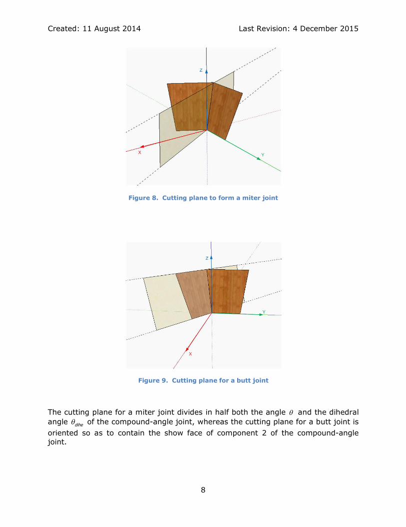
Figure 8. Cutting plane to form a miter joint

Figure 9. Cutting plane for a butt joint

The cutting plane for a miter joint divides in half both the angle π and the dihedralangle diheπ of the compound-angle joint, whereas the cutting plane for a butt joint isoriented so as to contain the show face of component 2 of the compound-anglejoint.


9

3 Developmentofsetupanglesusingplanetrigonometry,vectorsandrotationmatrices

Here is what we envision needs to happen. We consider that the imaginary cutplane is attached to component 1. The showing face of this component (or of theboard or material that is to become component 1) with its associated cut planeneeds to be oriented on the surface of the table saw (or other cutting machine) sothat the cut plane passes through the plane of the saw blade. This requires thatthe saw blade be tilted and the miter gauge be adjusted to match the orientation ofthe cut plane. So, we rotate component 1 and its attached cut plane clockwiseabout the Y-axis through the angle S. Component then lies on the surface of thetable saw, and the rotated unit vector 1uθ will then equal the unit vector Zeθ along

the Z-axis. The cut plane will be at an angle to the surface of the table saw of/ 2dihedπ for a miter joint or angle dihedπ for a butt joint. We call the angle that the

cut plane makes with the surface of the table-saw surface the blade angle, and de-note it by BA°, measured in degrees. Thus, by combining Eqns. (8) and (10),measured counterclockwise from the surface of the saw table, the blade angle BA°satisfies

∋ (∋ (

2 2

cos / 2 sin , miter jointcos

cos sin cos , butt jointo

SBA

S S

π

π

< ,

(11)

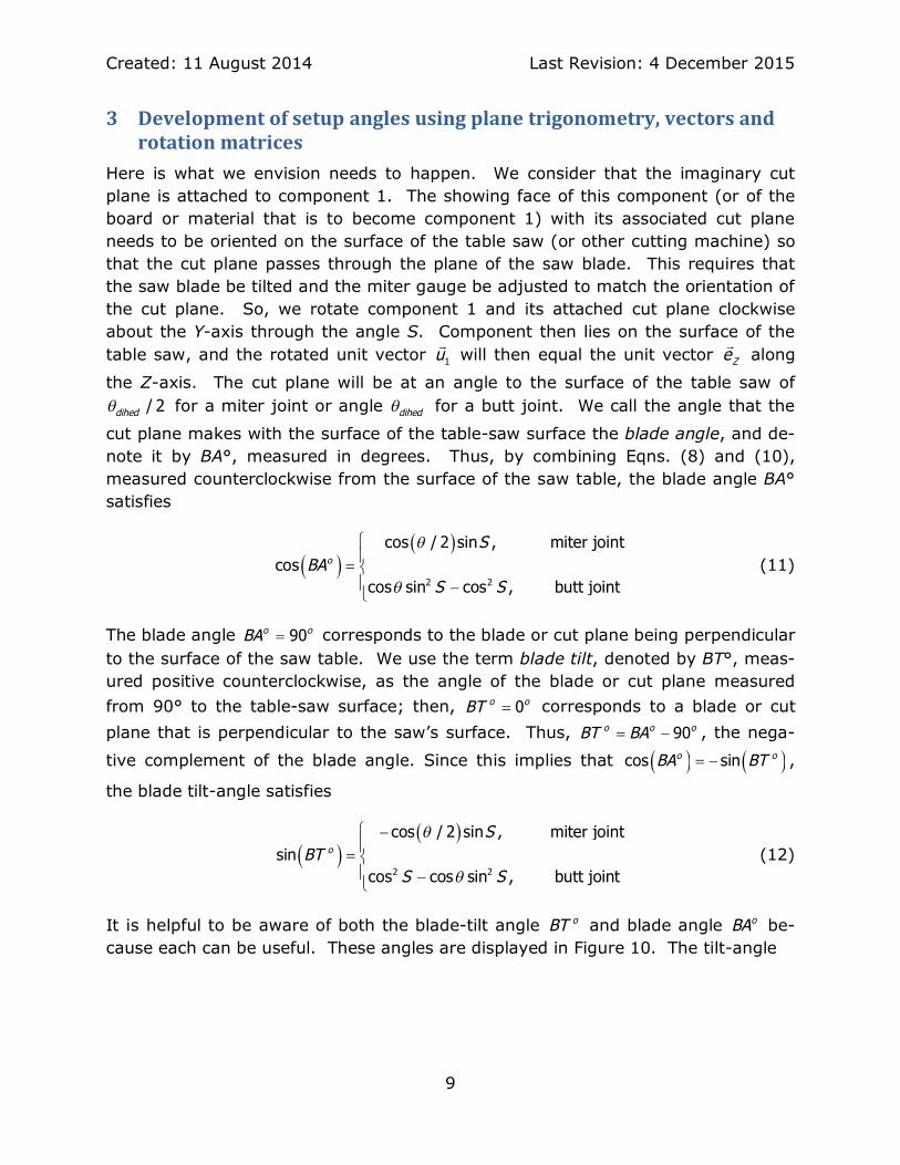
The blade angle 90o oBA < corresponds to the blade or cut plane being perpendicularto the surface of the saw table. We use the term blade tilt, denoted by BT°, meas-ured positive counterclockwise, as the angle of the blade or cut plane measuredfrom 90° to the table-saw surface; then, 0o oBT < corresponds to a blade or cutplane that is perpendicular to the saw’s surface. Thus, 90o o oBT BA< , , the nega-

tive complement of the blade angle. Since this implies that ∋ ( ∋ (cos sino oBA BT< , ,

the blade tilt-angle satisfies

∋ (∋ (

2 2

cos / 2 sin , miter jointsin

cos cos sin , butt jointo

SBT

S S

π

π

,< ,

(12)

It is helpful to be aware of both the blade-tilt angle oBT and blade angle oBA be-cause each can be useful. These angles are displayed in Figure 10. The tilt-angle


10

Figure 10. Blade and blade-tilt angles

is useful because this is the angle displayed on the angle scale that is built intosaws made by many manufacturers. However, these scales are coarse, makingprecise settings difficult. Instead of using the saw’s angle scale when more precisesettings are needed, it is convenient to set an auxiliary tool, such as a bevel gauge,to the desired blade angle oBA using an accurate protractor. The bevel gauge isthen placed on the table and the blade adjusted to match its angle. An alternativethat can be even more precise is to print onto regular printer paper a right trianglewith one of the acute angles being oBA . The printer paper is then glued to a heavycard stock backing, which is cut to form a triangular template that is used to set theblade to angle oBA .

A rotation of the combined component 1 and its cut plane around the Z-axis is alsoneeded to bring the cut plane into the plane of the tilted saw blade. That angle isthe required miter-gauge setting. This we identify in the following way. A unit vec-tor is constructed along the line where the two components meet. This unit vectoris rotated clockwise through an angle S around the Y-axis along with component 1and its attached cut plane. The resulting vector is then rotated around the Z-axisthrough an angle that yields a vector with an X component of zero. The angle re-quired to accomplish yields the miter-gauge angle.

The vector that results by forming the cross product between 1uθ and 2uθ ,


11

∋ (1 22

sin sin coscos sin cos sin cos sin

sin sindihed

S Su u S S S S n

S

ππ π

π

, ≥ < , , <

θθ θ, (13)

lies in the cutting plane (for both miter and butt joints) along the mating line ofcomponents 1 and 2; nθ is a unit vector that lies along the mating line. Clockwiserotation of this vector about the Y-axis through angle S yields

∋ ( 1 2

2

2 3

2 2

cos 0 sin sin sin cos0 1 0 cos sin cos sin cos

sin 0 cos sin sin

sin sin cos sin sincos sin cos sin cos

sin sin cos sin sin cos

sin sincos

Yw R S u u

S S S SS S S S

S S S

S S SS S S S

S S S S

S

ππ

π

π ππ

π π

π

< , ≥

, , < , ,

, , < , , , ∗

,< ,

θ θ θ

2 2sin cos sin cos .

sin sin cos sin sin cosS S S S

S S S Sπ

π π

, , ∗

(14)

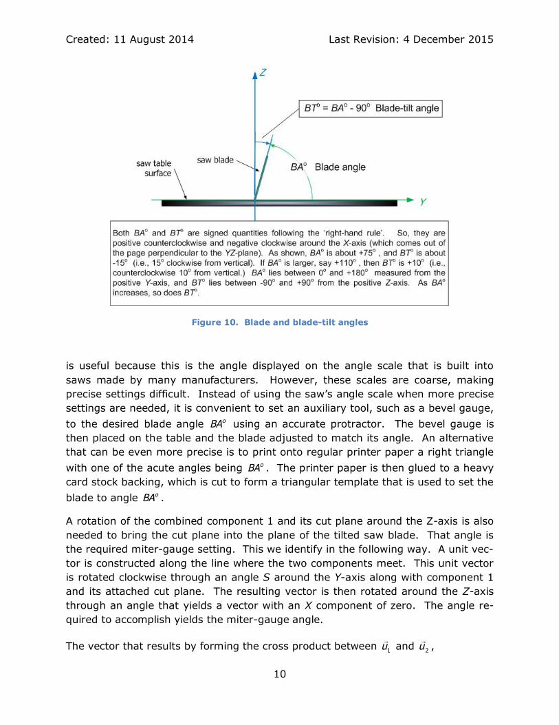
The vector wθ is in the XY-plane aligned along the mating line of the two compo-nents, as shown in Figure 11 for component 1.

Figure 11. Component 1 positioned flat on the XY-plane


12

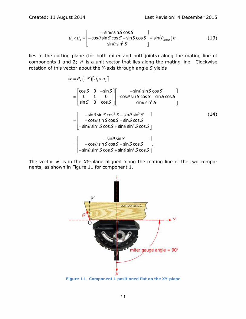
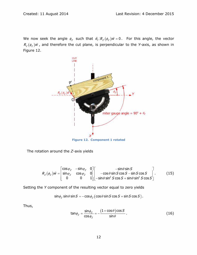
We now seek the angle Zε such that ∋ ( 0Y Z Ze R wε <θ θÿ . For this angle, the vector

∋ (Z ZR wεθ, and therefore the cut plane, is perpendicular to the Y-axis, as shown in

Figure 12.

Figure 12. Component 1 rotated

The rotation around the Z-axis yields

∋ (2 2

cos sin 0 sin sinsin cos 0 cos sin cos sin cos

0 0 1 sin sin cos sin sin cos

Z Z

Z Z Z Z

SR w S S S S

S S S S

ι ι πε ι ι π

π π

, , < , ,

, ∗

θ. (15)

Setting the Y component of the resulting vector equal to zero yields

∋ (sin sin sin cos cos sin cos sin cosZ ZS S S S Sε π ε π< , ∗ .

Thus,∋ (1 cos cossintan

cos sinZ

ZZ

Sπεε

ε π∗

< < , . (16)


13

We now use the half-angle formulas ∋ ( ∋ (sin 2sin / 2 cos / 2π π π< and

∋ (21 cos 2cos / 2π π∗ < to obtain

∋ (costan

tan / 2zSε

π< , . (17)

The miter-gauge angle5, shown as oMG in Fig. 12, is given in terms of Zε by

90o oZMG ε< ∗ , which can be less or greater than 90° depending on the sign of Zε .

Thus, from Eqn. (17)

∋ ( ∋ ( ∋ (tan / 21tan tan 90tan cos

o oZ

ZMG

Sπ

εε

< ∗ < , < . (18)

Care is needed with the inverse tangent-function when determining the miter-gauge angle with this expression. The version of the inverse tangent-function to beused is:

∋ (∋ (arctan2 tan / 2 ,cosoMG Sπ< , (19)

where

∋ (

∋ (∋ (∋ (

arctan / , 0arctan / 180 , 0, 0arctan / 180 , 0, 0arctan2 ,90 , 0, 090 , 0, 0

undefined, 0, 0

o

o

o

o

y x xy x y xy x y xy x

y xy xy x

=

∗ ″ ; , ; ;<

= <, ; <

< <

(20)

Expressions for the blade and miter setup angles for compound-angle joints are de-veloped in this section using plane trigonometry, vectors and rotation matrices.Eqn. (12) is the expression for the blade-tilt angle, and Eqn. (18) is for the miter-gauge angle. In each of these expressions, the angle π is the angle in the XY-plane between the two components forming the compound-angle joint, as shown in

5 Note here that the miter-gauge angle oMG is measured as an angle about the Z-axis, with90o corresponding to the miter gauge set perpendicular to the plane of the cutting blade.The scale on miter-gauge tools are often marked with 90o corresponding to perpendicularto the cutting blade and, further, the scale is marked symmetrically either side of 90o .Care is therefore needed when converting oMG into scale readings.


14

Figure 6. Expressions for the setup angles are developed in another way in thenext section.

4 DevelopmentofsetupanglesusingsphericaltrigonometryBill Gottesman formulated the ideas for this alternative development by usingspherical trigonometry. Bill routinely uses spherical trigonometry for his designs ofnovel sundials, and the motivation for pursuing this development originated from aconversation between the authors at the Annual Conference of the North AmericanSundial Society held in Indianapolis, IN, in August 2014. We offer both the devel-opment of the previous section based on plane trigonometry and the developmentof this section using spherical trigonometry because each conceptualization pro-vides its own distinct insights that may be helpful to others interested in compound-angle joinery.

Spherical trigonometry plays an important role in many applications, including nav-igation, astronomy, and surveying. We will indicate its use in compound-anglejoinery. First some terminology. A circle is formed at the intersection of a planewith the surface of a sphere. Such a circle is called a great circle when the inter-secting plane passes through the center of the sphere; otherwise it is called a smallcircle. For example, the equator is a great circle on the earth’s surface (when theearth is approximated as a sphere), dividing the earth into its northern and south-ern hemispheres. Great circles partition the earth into zones of longitude, andsmall circles partition it into zones of latitude. Spherical trigonometry deals withpolygonal shapes that occur on the surface of a sphere when multiple great circlesintersect. As seen in Fig. 10, three great circles can intersect to form a spherical

Figure 13. Spherical triangle


15

triangle. Four can form a spherical square, five a spherical pentagon, etc. Spheri-cal pentagons and hexagons are the shapes seen on the surface of the soccer ballin Fig. 11. Three planes intersecting to form a spherical triangle can help to explaintable-saw setup angles when forming objects requiring compound angle joinery.

Fig. 10 shows three great circles that intersect to form a spherical triangle withvertices labeled A, B and C. The angle C-A-B at vertex A is also referred to as theangle A, which is measured in angular units of degrees or radians; likewise for theangles at vertices B and C. The three sides of the spherical triangle are also meas-ured in angular units. The side opposite of the vertex A is labeled a. The size of ais that of the angle B-O-C. Similarly, the sizes of the sides labeled b and c arethose of the angles A-O-C and A-O-B, respectively. A plane that is tangent to thesphere at the point of vertex A is perpendicular to the radial line O-A. Therefore,any line in that plane which passes through the point of tangency is perpendicularto that radial line. In particular, consider two lines in the tangent plane, one that isalso in the plane defined by A-O-B and the other in the plane defined by A-O-C.The angle between these lines is the dihedral angle of the two intersecting planescontaining A-O-B and A-O-C. Thus, the angle A associated with vertex A is the di-hedral angle of the two planes that intersect along the radial line O-A.

Spherical trigonometry deals with relationships between the six angles A, B, C, a, band c. Here, we summarize these relationships found in standard textbooks [8, 9,11] and many websites [7, 10]. The fundamental equations, called the law of co-sines, are:

Figure 14. Soccer ball


16

cos cos cos sin sin cos


cos cos cos sin sin cos .

< ∗

< ∗

< ∗

a b c b c A

b a c a c B

c a b a b C

(21)

Six angles are associated with any spherical triangle. These fundamental equationspermit the determination of all six by knowing any three of them. Manipulation ofthese fundamental equations yields:



cos cos cos sin sin cos .

< , ∗

< , ∗

< , ∗

A B C B C a

B C A C A b

C A B A B c

(22)

Daniel Wenger gives a derivation of the law of cosines by using the rotation matri-ces of Section 2.1. Many other relationships can be derived from the law of cosinesby using trigonometric identities [8-11].

4.1 Placingacompound-anglejointinthegeometryofsphericaltrigonome-try

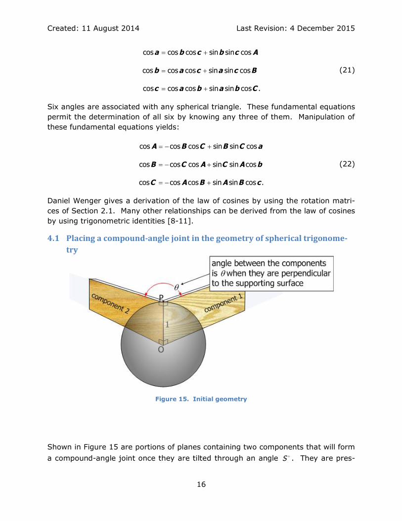
Figure 15. Initial geometry

Shown in Figure 15 are portions of planes containing two components that will forma compound-angle joint once they are tilted through an angle S ν . They are pres-


17

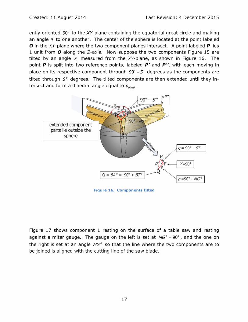
ently oriented 90o to the XY-plane containing the equatorial great circle and makingan angle π to one another. The center of the sphere is located at the point labeledO in the XY-plane where the two component planes intersect. A point labeled P lies1 unit from O along the Z-axis. Now suppose the two components Figure 15 aretilted by an angle S measured from the XY-plane, as shown in Figure 16. Thepoint P is split into two reference points, labeled P’ and P’’, with each moving inplace on its respective component through 90 S,ν ν degrees as the components aretilted through oS degrees. The tilted components are then extended until they in-tersect and form a dihedral angle equal to dihedπ .

Figure 16. Components tilted

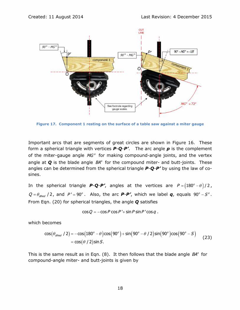
Figure 17 shows component 1 resting on the surface of a table saw and restingagainst a miter gauge. The gauge on the left is set at 90o oMG < , and the one onthe right is set at an angle oMG so that the line where the two components are tobe joined is aligned with the cutting line of the saw blade.


18

Figure 17. Component 1 resting on the surface of a table saw against a miter gauge

Important arcs that are segments of great circles are shown in Figure 16. Theseform a spherical triangle with vertices P-Q-P’. The arc angle p is the complementof the miter-gauge angle oMG for making compound-angle joints, and the vertexangle at Q is the blade angle oBA for the compound miter- and butt-joints. Theseangles can be determined from the spherical triangle P-Q-P’ by using the law of co-sines.

In the spherical triangle P-Q-P’, angles at the vertices are ∋ (180 / 2oP π< , ,

/ 2dihedQ π< , and ' 90oP < . Also, the arc P-P’, which we label q, equals 90o oS, .

From Eqn. (20) for spherical triangles, the angle Q satisfies

cos cos cos ' sin sin ' cosQ P P P P q< , ∗ .

which becomes

∋ ( ∋ ( ∋ ( ∋ ( ∋ ( ∋ (∋ (

cos / 2 cos 180 cos 90 sin 90 / 2 sin 90 cos 90

cos / 2 sin .

o o o o odihed S

S

π π π

π

< , , ∗ , ,

< (23)

This is the same result as in Eqn. (8). It then follows that the blade angle oBA forcompound-angle miter- and butt-joints is given by


19

∋ (∋ (

2 2

cos / 2 sin , miter jointcos

cos sin cos , butt jointo

SBA

S S

π

π

< ,

(24)

This is the same as Eqn. (11). To determine the arc P’-Q, which we label p, weagain use the cosine law, Eqn. (21), to obtain

cos cos 'cos sin ' sin cosP P Q P Q p< , ∗ .

Thus,

∋ ( ∋ ( ∋ ( ∋ ( ∋ (∋ (

cos 90 / 2 cos 90 cos / 2 sin 90 sin / 2 cos

sin / 2 cos .dihed dihed

dihed

p

p

π π π

π

, < , ∗

<

ν ν ν

(25)

The miter-gauge angle for a compound-angle joint is equal to the complement ofthe arc-angle p, so

∋ ( ∋ ( ∋ (∋ (

sin / 2cos 90 sin

sin / 2o o o

dihedMG MG

ππ

, < < . (26)

This is an alternative expression for the miter-gauge angle from that in Eqn. (18).To see that the two expressions yield identical results requires some manipulationsusing trigonometric identities. Start by squaring Eqn. (26) and using Eqn. (23) toget

∋ ( ∋ ( ∋ (∋ (

∋ (∋ (

2 2 22 2

2 2 2 2

sin / 2 cos / 2 coscos 1 sin 1

1 cos / 2 sin 1 cos / 2 sino o S

MG MGS S

π ππ π

< , < , <, ,

.

Then,

∋ (∋ ( ∋ ( ∋ (

∋ (∋ (2 2 2

22 2 22

sin sin / 2 tan / 2tan

cos / 2 cos coscos

oo

o

MGMG

S SMGπ π

π< < < .

The square root then shows that Eqns. (26) and (18) are equivalent expressions forthe miter-gauge angle for forming a compound-angle joint.

5 SummaryofResults

Assume that the two components of a compound-angle joint meet at an angle π inthe XY-plane. A special case arises when the components are part of a box whoseshape in the XY-plane is a regular polygon (eg. square, hexagon) having N sides;


20

then ∋ (180 2 /N Nπ < ,ν . The miter-gauge angle MG ν is referenced to be 90ν when it

is perpendicular to the plane of the cutting blade, and the blade-tilt angle BT ν isreferenced from the XY-plane (surface of the saw table). Assume that the compo-nent parts slope S ν from the XY-plane. Then, the blade-tilt angle satisfies

∋ (∋ (

2 2

cos / 2 sin , miter jointsin

cos cos sin , butt joint.o

SBT

S S

π

π

,< ,

(27)

The dihedral angle dihedπ of the compound-angle joint is equal to 2 *BAν for a miter

joint and BAν for a butt joint. The miter-gauge angle satisfies∋ (tan / 2

tancos

oMGS

π< , (28)

which is Eqn. (18). Alternatively, and equivalently, the miter-gauge angle also sat-isfies

∋ ( ∋ (∋ (

sin / 2sin

sin / 2o

dihedMG

ππ

< , (29)

which is Eqn. (26). For regular polygonal boxes having N sides, ∋ (180 2 /o N Nπ < , ,these expressions become

∋ (2 2

cos 90 ( 2) / sin , miter jointsin

cos cos 90 ( 2) / sin , butt joint

o

o

o

N N SBT

S N N S

, , <

, ,

(30)

and∋ (tan 90 2 /

tancos

oo

N NMG

S , < (31)

or, alternatively

∋ ( ∋ (∋ (

sin 90 2 /sin

sin / 2

oo

dihed

N NMG

π

, < , (32)

where / 2 odihed BAπ < for a miter joint in Eqn. (29).


21

6 ComputerImplementations

6.1 InternetImplementationsA number of Internet sites provide interactive calculators that produce values forsaw setup angles for compound-angle joinery. References [3] and [4] are exam-ples.

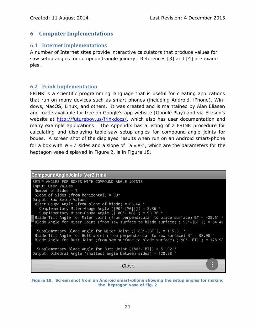
6.2 FrinkImplementationFRINK is a scientific programming language that is useful for creating applicationsthat run on many devices such as smart-phones (including Android, iPhone), Win-dows, MacOS, Linux, and others. It was created and is maintained by Alan Eliasenand made available for free on Google’s app website (Google Play) and via Eliasen’swebsite at http://futureboy.us/frinkdocs/, which also has user documentation andmany example applications. The Appendix has a listing of a FRINK procedure forcalculating and displaying table-saw setup-angles for compound-angle joints forboxes. A screen shot of the displayed results when run on an Android smart-phonefor a box with 7N < sides and a slope of 83S < ν , which are the parameters for theheptagon vase displayed in Figure 2, is in Figure 18.

Figure 18. Screen shot from an Android smart-phone showing the setup angles for makingthe heptagon vase of Fig. 2


22

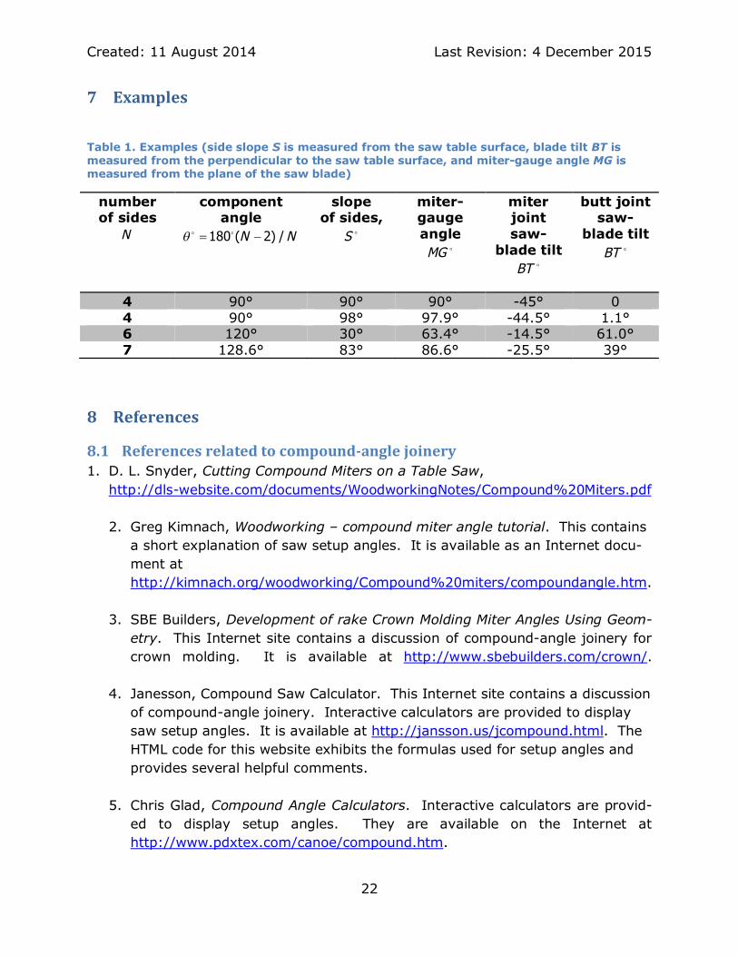
7 Examples

Table 1. Examples (side slope S is measured from the saw table surface, blade tilt BT ismeasured from the perpendicular to the saw table surface, and miter-gauge angle MG ismeasured from the plane of the saw blade)

numberof sides

N

componentangle

180 ( 2) /N Nπ < ,ν ν

slopeof sides,

S ν

miter-gaugeangleMG ν

miterjointsaw-

blade tiltBT ν

butt jointsaw-

blade tiltBT ν

4 90° 90° 90° -45° 04 90° 98° 97.9° -44.5° 1.1°6 120° 30° 63.4° -14.5° 61.0°7 128.6° 83° 86.6° -25.5° 39°

8 References

8.1 Referencesrelatedtocompound-anglejoinery1. D. L. Snyder, Cutting Compound Miters on a Table Saw,

http://dls-website.com/documents/WoodworkingNotes/Compound%20Miters.pdf

2. Greg Kimnach, Woodworking – compound miter angle tutorial. This containsa short explanation of saw setup angles. It is available as an Internet docu-ment athttp://kimnach.org/woodworking/Compound%20miters/compoundangle.htm.

3. SBE Builders, Development of rake Crown Molding Miter Angles Using Geom-etry. This Internet site contains a discussion of compound-angle joinery forcrown molding. It is available at http://www.sbebuilders.com/crown/.

4. Janesson, Compound Saw Calculator. This Internet site contains a discussionof compound-angle joinery. Interactive calculators are provided to displaysaw setup angles. It is available at http://jansson.us/jcompound.html. TheHTML code for this website exhibits the formulas used for setup angles andprovides several helpful comments.

5. Chris Glad, Compound Angle Calculators. Interactive calculators are provid-ed to display setup angles. They are available on the Internet athttp://www.pdxtex.com/canoe/compound.htm.


23

6. Compound Miter Template Generator. An interactive calculator is provided todisplay setup angles and print templates. It is available on the Internet athttp://www.blocklayer.com/compoundmitereng.aspx.

8.2 Referencesrelatedtosphericaltrigonometry

7. Daniel L. Wenger, Derivation of the Spherical Law of Cosines and Sines usingRotation Matrices. Available on the Internet athttp://www.wengersundial.com/new/resources/Mathematics/SpherTrig.pdf.

8. Daniel A. Murray, Spherical Trigonometry, Longmans, Green and Co., 1908.This is available as an Internet Archive Organization eBook athttps://archive.org/details/sphericaltrigono00murrrich.

9. I. Todhunter, Spherical Trigonometry: For the Use of Colleges and Schools,With Numerous Examples, McMillan and Co., 1886. This is available as aProject Gutenberg eBook at http://www.gutenberg.org/files/19770/19770-pdf.pdf.

10.Spherical Trigonometry, an Internet Wikipedia resourcehttp://en.wikipedia.org/wiki/Spherical_trigonometry

11.A. Albert Klaf, Trigonometry Refresher, Dover Publications Inc., 2005. Thiscontains a chapter on spherical trigonometry.

9 Appendices

9.1 NotationTwo forms of multiplication for vector-valued quantities are used in development.These are defined as follows. Let aθ and b

θ be three-dimensional vectors,

1 1

2 2

3 3

, anda b

a a b ba b

< <

θθ.

The dot product, denoted by a bθθÿ , is a number defined by

1 1 2 2 3 3a b a b a b a b< ∗ ∗θθÿ .

The cross product, denoted by a b≥θθ, is a vector defined by


24

2 3 3 2

3 1 1 3

1 2 2 1

a b a ba b a b a b

a b a b

, ≥ < ,

,

θθ.

Discussion of these products and some of their properties is given at the websites:

http://en.wikipedia.org/wiki/Dot_producthttp://en.wikipedia.org/wiki/Cross_product

A property of the dot product that we use is:

cos aba b a b π<θ θθ θÿ

where 2 2 2X Y Za a a a< ∗ ∗

θ and abπ is the angle between the vectors aθ and b

θ. Also,

for the cross product,

sin aba b a b nπ≥ <θ θθ θ θ

where nθ is a unit vector that is perpendicular to the plane containing aθ and bθ and

oriented in a direction that is consistent with the right-hand rule.

9.2 Frinkprocedureforcalculatingsetupangles

---------- start FRINK procedure -----------

// Calculates table saw settings for

//cutting sides of an multi-sided vessel

//having sides that slope.

// N number of sides

// S angle of the sides from horizontal (degrees)

// MG miter gauge angle (degrees) from plane of blade

// BT blade tilt angle (degrees) from saw surface

//Created By: D. L. Snyder 26 Feb 2011

//Revised: 27 Oct 2013 (added output of dihedral angle)

//Revised: 29 Aug 2014 (added butt joints, corrected Corner_Angle)

//Revised: 1 Dec 2015 (corrected coordinates for miter guage angle)

//

//start.........


25

//user inputs

[N, S] = input["Vessel or Box Information",

["Number of sides",

"Angle of sides from horizontal (degrees)"]]

//evaluate constants

S_deg = eval[S]

N_num = eval[N]

Corner_Angle = 180*(N_num-2)/N_num

a1 = sin[S_deg degrees]

a2 = cos[Corner_Angle/2 degrees]

b1 = cos[S_deg degrees]

b2 = tan[Corner_Angle/2 degrees]

//evaluate outputs

BT_MiterJoint = arcsin[-a1*a2]

BA_MiterJoint = pi/2-abs[BT_MiterJoint] //complement of BT_MiterJoint

BA_MJsupplement = pi - abs[BA_MiterJoint]

//

BA_ButtJoint = 2*BA_MiterJoint

BA_BJsupplement = pi - abs[BA_ButtJoint]

BT_ButtJoint = abs[pi/2 - abs[BA_ButtJoint]] //complement ofBA_ButtJoint

//

MG = arctan[b2,b1] //angle from plane of blade

MGcomplement = abs[pi/2 - abs[MG]]

MGsupplement = abs[pi - abs[MG]]

//

DihedralAngle = BA_ButtJoint

// display results

println[" SETUP ANGLES FOR BOXES WITH COMPOUND-ANGLE JOINTS"]

println[" Input: User Values"]

println[" Number of Sides = " + N_num]

println[" Slope of Sides (from horizontal) = " + eval[S] + "\u00B0"]

// '\u00B0' is the unicode for the degree symbol

println[" Output: Saw Setup Values"]


26

println[" Miter Gauge Angle (from plane of blade) = " + format[MG,"\u00B0",2]]

println[" Complementary Miter-Gauge Angle (|90\u00B0-|MG||]) = " +format[MGcomplement,"\u00B0", 2]]

println[" Supplementary Miter-Gauge Angle (|180\u00B0-|MG||) = " +format[MGsupplement,"\u00B0", 2]]

println[" Blade Tilt Angle for Miter Joint (from perpendicular to blade surface)BT = " + format[BT_MiterJoint,"\u00B0", 2]]

println[" Blade Angle for Miter Joint (from saw surface to blade surface)(|90\u00B0-|BT||) = " + format[BA_MiterJoint,"\u00B0", 2]]

println[" Supplementary Blade Angle for Miter Joint (|180\u00B0-|BT||) = "+ format[BA_MJsupplement,"\u00B0", 2]]

println[" Blade Tilt Angle for Butt Joint (from perpendicular to saw surface)BT = " + format[BT_ButtJoint,"\u00B0", 2]]

println[" Blade Angle for Butt Joint (from saw surface to blade surface)(|90\u00B0-|BT||) = " + format[BA_ButtJoint,"\u00B0", 2]]

println[" Supplementary Blade Angle for Butt Joint (180\u00B0-|BT|) = " +format[BA_BJsupplement,"\u00B0", 2]]

println[" Output: Dihedral Angle (smallest angle between sides) = " +format[DihedralAngle,"\u00B0", 2]]

//..........end

---------- end FRINK procedure -----------

1 introduction - donald l. snyderdls-website.com/.../compoundanglejoinery.pdf · compound-angle...

Documents