1 introduction to tddft · = 27.21 ev = 627.5 kcal/mol), and times in units of 2.419×10⁻¹⁷ s....
TRANSCRIPT

1 Introduction to TDDFT
Eberhard K. U. Gross and Neepa T. Maitra
1.1 Introduction
Correlated electron motion plays a significant role in the spectra describedin the previous chapters. Further, placing an atom, molecule or solid in astrong laser field reveals fascinating non-perturbative phenomena, such asnon-sequential multiple-ionization (see Chapter (IV.5), whose origins lie inthe subtle ways electrons interact with each other. The direct approach totreat these problems is to solve the (non-relativistic) time-dependent Schrodingerequation for the many-electron wavefunction Ψ(t):
H(t)Ψ(t) = i∂Ψ(t)
∂t, H(t) = T + Vee + Vext(t) (1.1)
for a given initial wavefunction Ψ(0). Here, the kinetic energy and electron-electron repulsion, are, respectively:
T = −1
2
N∑
i=1
∇2i , and Vee =
1
2
N∑
i6=j
1
|ri − rj |, (1.2)
and the “external potential” represents the potential the electrons experiencedue to the nuclear attraction and due to any field applied to the system (e.g.laser):
Vext(t) =
N∑
i=1
vext(ri, t) . (1.3)
For example, vext(ri, t) can represent the Coulomb interaction of the electronswith a set of nuclei, possibly moving along some classical path,
vext(r, t) = −Nn∑
ν=1
Zν
|r −Rν(t)| , (1.4)
where Zν and Rν denote the charge and position of the nucleus ν, and Nn
stands for the total number of nuclei in the system. This may be useful tostudy, e.g., scattering experiments, chemical reactions, etc. Another example

2 E. K. U. Gross and N. T. Maitra
is the interaction with external fields, e.g. for a system illuminated by a laserbeam we can write, in the dipole approximation,
vext(r, t) = E f(t) sin(ωt)r ·α−Nn∑
ν=1
Zν
|r −Rν |, (1.5)
where α, ω and E are the polarization, the frequency and the amplitude ofthe laser, respectively. The function f(t) is an envelope that describes thetemporal shape of the laser pulse. We use atomic units (e2 = ~ = m = 1)throughout this chapter; all distances are in Bohr, energies in Hartrees (1 H= 27.21 eV = 627.5 kcal/mol), and times in units of 2.419× 10⁻¹⁷ s.
Solving Eq. (1.1) is an exceedingly difficult task. Even putting aside time-dependence, the problem of finding the ground-state scales exponentially withthe number of electrons. Moreover, Ψ contains far more information than onecould possibly need or even want. For example, consider storing the groundstate of the oxygen atom, and for simplicity, disregard spin. Then Ψ dependson 24 coordinates, three for each of the eight electrons. Allowing ourselves amodest ten grid-points for each coordinate, means that we need 1024 num-bers to represent the wavefunction. Assuming each number requires one byteto store, and that the capacity of a DVD is 1010 bytes, we see that 1014
DVD’s are required to store just the ground-state wavefunction of the oxy-gen atom, even on a coarse grid. Physically, we are instead interested inintegrated quantities, such as one- or two-body probability-densities, which,traditionally can be extracted from this foreboding Ψ . However, a methodthat could yield such quantities directly, by-passing the need to calculate Ψ ,would be highly attractive. This is the idea of density-functional theories. Infact, in 1964, Hohenberg and Kohn [Hohenberg 1964], proved that all observ-able properties of a static many-electron system can be extracted exactly, inprinciple, from the one-body ground-state density alone. Twenty years later,Runge and Gross extended this to time-dependent systems, showing that allobservable properties of a many-electron system, beginning in a given ini-tial state Ψ(0), may be extracted from the one-body time-dependent densityalone [Runge 1984]. What has made (TD)DFT so incredibly successful is theKohn-Sham system: the density of the interacting many-electron system isobtained as the density of an auxiliary system of non-interacting fermions,living in a one-body potential. The exponential scaling with system-size thatthe solution to Eq. (1.1) requires is replaced in TDDFT by the much gen-tler N3 or N2 (depending on the implementation) scaling [Marques 2006b]),opening the door to the quantum mechanical study of much larger systems,from nanoscale devices to biomolecules. (See Chapters (V.1)–(V.4) for detailson the numerical issues). Although the ground-state and time-dependent the-ories have a similar flavour, and modus operandi, their proofs and functionalsare quite distinct.
Before we delve into the details of the fundamental theorems of TDDFTin the next section, we make some historical notes. As early as 1933, Bloch

1 Introduction to TDDFT 3
proposed a time-dependent Thomas-Fermi model [Bloch 1933]. Ando [Ando1977a, Ando 1977b], Peuckert [Peuckert 1978] and Zangwill and Soven [Zangwill1980a, Zangwill 1980b] ran the first time-dependent KS calculations, assum-ing a TDKS theorem exists. They treated the linear density response to atime-dependent external potential as the response of non-interacting electronsto an effective time-dependent potential. Ando calculated resonance energyand absorption lineshapes for intersubband transitions on the surface of sili-con, while Peuckert and Zangwill and Soven studied rare-gas atoms. In anal-ogy to ground-state KS theory, this effective potential was assumed to containan exchange-correlation (xc) part, vxc(r, t), in addition to the time-dependentexternal and Hartree terms. Peuckert suggested an iterative scheme for thecalculation of vxc, while Ando, Zangwill and Soven adopted the functionalform of the static exchange-correlation potential in LDA. Significant stepstowards a rigorous foundation of TDDFT were taken by Deb and Ghosh[Deb 1982, Ghosh 1982, Ghosh 1983a, Ghosh 1983b] for time-periodic po-tentials and by Bartolotti [Bartolotti 1981, Bartolotti 1982, Bartolotti 1984,Bartolotti 1987] for adiabatic processes. These authors formulated and ex-plored Hohenberg-Kohn and KS type theorems for the time-dependent den-sity for these cases. Modern TDDFT is based on the general formulation ofRunge and Gross [Runge 1984].
TDDFT is being used today in an ever-increasing range of applications towidely-varying systems in chemistry, biology, solid-state physics, and materi-als science. We end the introduction by classifying these into four areas. First,the vast majority of TDDFT calculations today lie in spectroscopy (Chap-ters I.2–I.3 earlier), yielding response and excitations of atoms, molecules andsolids. The laser field applied to the system, initially in its ground-state, isweak and perturbation theory applies. We need to know only the exchange-correlation potential in the vicinity of the ground-state, and often (but notalways), formulations directly in frequency-domain are used (Chapter II.4)and later in this chapter). Overall, results for excitation energies tend to befairly good (few tenths of an eV error, typically) but depend significantly onthe system and type of excitation considered, e.g. the errors for long-rangecharge-transfer excitations can be ten times as large. For solids, to obtainaccurate optical absorption spectra of insulators needs functionals more so-phisticated than the simplest ones (ALDA), however ALDA does very wellfor electron-energy-loss spectra. We shall return to the general performanceof TDDFT for spectra in Sect. 1.8.
The second class of applications is real-time dynamics in non-perturbativefields. The applied electric field is comparable to, or greater than, the staticelectric field due to the nuclei. Fascinating and subtle electron interactioneffects can make the “single active electron” picture often used for theseproblems break down. For dynamics in strong fields, it is pushing today’scomputational limits for correlated wavefunction methods to go beyond oneor two electrons in three-dimensions, so TDDFT is particularly promising in

4 E. K. U. Gross and N. T. Maitra
this regime. However, the demands on the functionals for accurate results canbe challenging. Chapter (IV.5) discusses many interesting phenomena, thatreveal fundamental properties of atoms and molecules. Also under this um-brella are coupled electron-ion dynamics. For example, applying a laser pulseto a molecule or cluster, drives both the electronic and nuclear system out ofequilibrium; generally their coupled motion is highly complicated, and vari-ous approximation schemes to account for electronic-nuclear “back-reaction”have been devised. Often in photochemical applications, the dynamics aretreated beginning on an excited potential energy surface; that is, the dynam-ics leading to the initial electronic excitation is not explicitly treated butinstead defines the initial state for the subsequent field-free dynamics of thefull correlated electron and ion system. We refer the reader to Chapters IV.1,IV.2 and IV.3 for both formal and practical discussions on how to treat thischallenging problem.
The third class of applications returns to the ground-state: based on thefluctuation-dissipation theorem, one can obtain an expression for the ground-state exchange-correlation energy from a TDDFT response function, as isdiscussed in Chapter III.6. Such calculations are significantly more computa-tionally demanding than usual ground-state calculations but provide a nat-ural methodology for some of the most difficult challenges for ground-stateapproximations, in particular van der Waal’s forces. We refer the reader toChapters III.6 and III.7 for a detailed discussion.
The fourth class of applications is related to viscous forces arising fromelectron-electron interactions in very large finite systems, or extended systemssuch as solids. Consider an initial non-equilibrium state in such a system, cre-ated, for example, by a laser pulse that is then turned off. For a large enoughsystem, electron interaction subsequently relaxes the system to the ground-state, or to thermal equilibrium. Relaxation induced by electron-interactioncan be in principle exactly captured in TDDFT, but for a theoretically con-sistent formulation, one should go beyond the most commonly used approxi-mations. A closely related approach is time-dependent current-density func-tional theory (TDCDFT) (Sect. 1.4.4 and Chapter VI.2, where an xc vector-potential provides the viscous force [D’Agosta 2006, Ullrich 2006b]. Dissipa-tion phenomena studied so far, using either TDDFT or TDCDFT, includeenergy loss in atomic collisions with metal clusters [Baer 2004], the stoppingpower of ions in electron liquids [Nazarov 2005, Hatcher 2008, Nazarov 2007],spin-Coulomb drag [d’Amico 2006, d’Amico 2010], and a hot electron prob-ing a molecular resonance at a surface [Gavnholt 2009]. Transport throughmolecular devices (Chapter IV.4 is an important subgroup of these applica-tions: how a system evolves to a steady-state after a bias is applied [Stefanucci2004a, Kurth 2005, Kurth 2010, Khosravi 2009, Stefanucci 2007, Koentopp2008, Zheng 2010]. In this problem, to account for coupling of electrons in themolecular wire to a “bath” of electrons in the leads, or to account for cou-pling to external phonon modes, one is led to the “open systems” analyses,

1 Introduction to TDDFT 5
reviewed in Chapters III.3 and III.4 [Gebauer 2004a, Burke 2005c, Yuen-Zhou 2010, Di Ventra 2007, Chen 2007, Appel 2009]. In [Ullrich 2002b] thelinear response of weakly disordered systems was formulated, embracing bothextrinsic damping (interface roughness and charged impurities) as well as in-trinsic dissipation from electron interaction.
The present chapter is organized as follows. Section 1.2 presents the proofof the fundamental theorem in TDDFT. Section 1.3 then presents the time-dependent KS equations, the “performers” of TDDFT. In Sect. 1.4 we discussseveral details of the theory, which are somewhat technical but important ifone scratches below the surface. Section 1.5 derives the linear response for-mulation, and the matrix equations which run the show for most of the appli-cations today. Section 1.6 briefly presents the equations for higher-order re-sponse, while Sect. 1.7 describes some of the approximations in use currentlyfor the xc functional. Finally, Sect. 1.8 gives an overview of the performanceand challenges for the approximations today.
1.2 One-to-one density-potential mapping
The central theorem of TDDFT (the Runge-Gross theorem) proves that thereis a one-to-one correspondence between the external (time-dependent) po-tential, vext(r, t), and the electronic one-body density, n(r, t), for many-bodysystems evolving from a fixed initial state Ψ0 [Runge 1984]. The density n(r, t)is the probability (normalized to the particle number N) of finding any oneelectron, of any spin σ, at position r:
n(r, t) = N∑
σ,σ2..σN
∫
d3r2 · · ·∫
d3rN |Ψ(rσ, r2σ2 · · · rNσN , t)|2 (1.6)
The implications of this theorem are enormous: if we know only the time-dependent density of a system, evolving from a given initial state, then thisidentifies the external potential that produced this density. The external po-tential completely identifies the Hamiltonian [the other terms (Eqs.(1.2)) aredetermined from the fact that we are dealing with electrons, with N being theintegral of the density of Eq. (1.6) over r]. The time-dependent Schrodingerequation can then be solved, in principle, and all properties of the systemobtained. That is, for this given initial-state, the electronic density, a func-tion of just three spatial variables and time, determines all other propertiesof the interacting many-electron system.
This remarkable statement is the analogue of the Hohenberg-Kohn the-orem for ground-state DFT, where the situation is somewhat simpler: thedensity-potential map there holds only for the ground-state, so there is notime-dependence and no dependence on the initial state. The Hohenberg-Kohn proof is based on the Rayleigh-Ritz minimum principle for the energy.A straightforward extension to the time-dependent domain is not possiblesince a minimum principle is not available in this case.
6 E. K. U. Gross and N. T. Maitra
Instead, the proof for a 1–1 mapping between time-dependent poten-tials and time-dependent densities is based on considering the quantum-mechanical equation of motion for the current-density, for a Hamiltonian ofthe form of Eqs. (1.1–1.3). The proof requires the potentials vext(r, t) to betime-analytic around the initial time, i.e. that they equal their Taylor-seriesexpansions in t around t = 0, for a finite time interval:
vext(r, t) =∞∑
k=0
1
k!vext,k(r)tk . (1.7)
The aim is to show that two densities n(r, t) and n′(r, t) evolving from acommon initial state Ψ0 under the influence of the potentials vext(r, t) andv′ext(r, t) are always different provided that the potentials differ by more than
a purely time-dependent function:
vext(r, t) 6= v′ext(r, t) + c(t) . (1.8)
The above condition is a physical one, representing simply a gauge-freedom.A purely time-dependent constant in the potential cannot alter the physics:if two potentials differ only by a purely time-dependent function, their re-sulting wavefunctions differ only by a purely time-dependent phase factor.Their resulting densities are identical. All variables that correspond to ex-pectation values of Hermitian operators are unaffected by such a purely time-dependent phase. There is an analogous condition in the ground-state proofof Hohenberg and Kohn. Equation (1.8) is equivalent to the statement thatfor the expansion coefficients vext,k(r) and v′
ext,k(r) [where, as in Eq. (1.7),
v′ext(r, t) =
∑∞k=0
1k!v
′ext,k(r)tk] there exists a smallest integer k ≥ 0 such
that
vext,k(r)− v′ext,k(r) =
∂k
∂tk[vext(r, t)− v′
ext(r, t)]
∣
∣
∣
∣
t=0
6= const. (1.9)
The initial state Ψ0 need not be the ground-state or any stationary stateof the initial potential, which means that “sudden switching” is covered bythe RG theorem. But potentials that turn on adiabatically from t = −∞, arenot, since they do not satisfy Eq. (1.7) (see also Sect. 1.5.3).
The first step of the proof demonstrates that the current-densities
j(r, t) = 〈Ψ(t)|j(r)|Ψ(t)〉 (1.10)
andj′(r, t) = 〈Ψ ′(t)|j(r)|Ψ ′(t)〉 (1.11)
are different for different potentials vext and v′ext. Here,
j(r) =1
2i
N∑
i=1
[∇iδ(r − ri) + δ(r − ri)∇i] (1.12)

1 Introduction to TDDFT 7
is the usual paramagnetic current-density operator. In the second step, useof the continuity equation shows that the densities n and n′ are different. Wenow proceed with the details.
Step 1 We apply the equation of motion for the expectation value of ageneral operator Q(t),
∂
∂t〈Ψ(t)|Q(t)|Ψ(t)〉 = 〈Ψ(t)|
(
∂Q
∂t− i[Q(t), H(t)]
)
|Ψ(t)〉 , (1.13)
to the current densities:
∂
∂tj(r, t) =
∂
∂t〈Ψ(t)|j(r)|Ψ(t)〉 =− i〈Ψ(t)|[j(r), H(t)]|Ψ(t)〉 (1.14a)
∂
∂tj′(r, t) =
∂
∂t〈Ψ ′(t)|j(r)|Ψ ′(t)〉 =− i〈Ψ ′(t)|[j(r), H ′(t)]|Ψ ′(t)〉, (1.14b)
and take their difference evaluated at the initial time. Since Ψ and Ψ ′ evolvefrom the same initial state
Ψ(t = 0) = Ψ ′(t = 0) = Ψ0 , (1.15)
and the corresponding Hamiltonians differ only in their external potentials,we have
∂
∂t[j(r, t)− j′(r, t)]
∣
∣
∣
∣
t=0
= −i〈Ψ0|[j(r), H(0)− H ′(0)]|Ψ0〉
= −n0(r)∇ [vext(r, 0)− v′ext(r, 0)] (1.16)
where n0(r) is the initial density. Now, if the condition (1.9) is satisfied fork = 0 the right-hand side of (1.16) cannot vanish identically and j andj′ will become different infinitesimally later than t = 0. If the smallest in-teger k for which Eq. (1.9) holds is greater than zero, we use Eq. (1.13)
(k + 1) times. That is, as for k = 0 above where we used Q(t) = j(r)
in Eq. (1.13), for k = 1, we take Q(t) = −i[j(r), H(t)]; for general k,
Q(t) = (−i)k[[[j(r), H(t)], H(t)]...H(t)]k meaning there are k nested com-mutators to take. After some algebra1:
(
∂
∂t
)k+1
[j(r, t)− j′(r, t)]
∣
∣
∣
∣
t=0
= −n0(r)∇wk(r) 6= 0 (1.17)
with
wk(r) =
(
∂
∂t
)k
[vext(r, t)− v′ext(r, t)]
∣
∣
∣
∣
t=0
. (1.18)
1 Note that Eq. (1.17) applies for all integers from 0 to this smallest k for whichEq. (1.9) holds, but not for integers larger than this smallest k.

8 E. K. U. Gross and N. T. Maitra
Once again, we conclude that infinitesimally later than the initial time,
j(r, t) 6= j′(r, t) . (1.19)
This first step thus proves that the current-densities evolving from the sameinitial state in two physically distinct potentials, will differ. That is, it provesa one-to-one correspondence between current-densities and potentials, for agiven initial-state.
Step 2 To prove the corresponding statement for the densities we use thecontinuity equation
∂n(r, t)
∂t= −∇ · j(r, t) (1.20)
to calculate the (k+2)nd time-derivative of the density n(r, t) and likewise ofthe density n′(r, t). Taking the difference of the two at the initial time t = 0and inserting Eq. (1.18) yields
(
∂
∂t
)k+2
[n(r, t)− n′(r, t)]
∣
∣
∣
∣
t=0
= ∇ · [n0(r)∇wk(r)] . (1.21)
Now, if there was no divergence-operator on the r.h.s., our task would becomplete, showing that the densities n(r, t) and n′(r, t) will become differentinfinitesimally later than t = 0. To show that the divergence does not renderthe r.h.s. zero, thus allowing an escape from this conclusion, we consider theintegral
∫
d3r n0(r)[∇wk(r)]2
= −∫
d3r wk(r)∇ · [n0(r)∇wk(r)] +
∮
dS · [n0(r)wk(r)∇wk(r)] , (1.22)
where we have used Green’s theorem. For physically reasonable potentials(i.e. potentials arising from normalizable external charge densities), the sur-face integral on the right vanishes [Gross 1990] (more details are given inSect. 1.4.1). Since the integrand on the left-hand side is strictly positiveor zero, the first term on the right must be strictly positive. That is, ∇ ·[n0(r)∇wk(r)] cannot be zero everywhere. This completes the proof of thetheorem.
We have shown that densities evolving from the same initial wavefunctionΨ0 in different potentials must be diffferent. Schematically, the Runge-Grosstheorem shows
Ψ0 : vext1−1←→ n . (1.23)
The backward arrow, that a given time-dependent density points to a singletime-dependent potential for a given initial state, has been proven above.The forward arrow follows directly from the uniqueness of solutions to thetime-dependent Schrodinger equation.

1 Introduction to TDDFT 9
Due to the one-to-one correspondence, for a given initial state, the time-dependent density determines the potential up to a purely time-dependentconstant. The wavefunction is therefore determined up to a purely-time-dependent phase, as discussed at the beginning of this section, and so can beregarded as a functional of the density and initial state:
Ψ(t) = e−iα(t)Ψ [n, Ψ0](t) . (1.24)
As a consequence, the expectation value of any quantum mechanical Hermi-tian operator Q(t) is a unique functional of the density and initial state (and,not surprisingly, the ambiguity in the phase cancels out):
Q[n, Ψ0](t) = 〈Ψ [n, Ψ0](t)|Q(t)|Ψ [n, Ψ0](t)〉 . (1.25)
We also note that the particular form of the Coulomb interaction did notenter into the proof. In fact, the proof applies not just to electrons, but toany system of identical particles, interacting with any (but fixed) particle-interaction, and obeying either fermionic or bosonic statistics.
In Sect. 1.4 we shall return to some details and extensions of the proof, butnow we proceed with how TDDFT operates in practice: the time-dependentKohn-Sham equations.
1.3 Time-dependent Kohn-Sham equations
Finding functionals directly in terms of the density can be rather difficult.In particular, it is not known how to write the kinetic energy as an explicitfunctional of the density. The same problem occurs in ground-state DFT,where the search for accurate kinetic-energy density-functionals is an activeresearch area. Instead, like in the ground-state theory, we turn to a non-interacting system of fermions called the Kohn-Sham (KS) system, definedsuch that it exactly reproduces the density of the true interacting system.A large part of the kinetic energy of the true system is obtained directly asan orbital-functional, evaluating the usual kinetic energy operator on the KSorbitals. (The rest, along with other many-electron effects, is contained inthe exchange-correlation potential.) All properties of the true system can beextracted from the density of the KS system.
Because the 1–1 correspondence between time-dependent densities andtime-dependent potentials can be established for any given interaction Vee,in particular also for Vee ≡ 0, it applies to the KS system. Therefore theexternal potential vKS[n;Φ0](r, t) of a non-interacting system reproducing agiven density n(r, t), starting in the initial state Φ0, is uniquely determined.The initial KS state Φ0 is almost always chosen to be a single Slater determi-nant of single-particle orbitals ϕ(r, 0) (but need not be); the only conditionon its choice is that it must be compatible with the given density. That is,it must reproduce the initial density and also its first time-derivative [from
10 E. K. U. Gross and N. T. Maitra
Eq. (1.20), see also Eqs. (1.29–1.30) shortly]. However, the 1–1 correspon-dence only ensures the uniqueness of vKS[n;Φ0] but not its existence for anarbitrary n(r, t). That is, the proof does not tell us whether a KS system existsor not; this is called the non-interacting v-representability problem, similar tothe ground-state case. We return to this question later in Sect. 1.4.2, but fornow we assume that vKS exists for the time-dependent density of the interact-
ing system of interest. Under this assumption, the density of the interactingsystem can be obtained from
n(r, t) =
N∑
j=1
|ϕj(r, t)|2 (1.26)
with orbitals ϕj(r, t) satisfying the time-dependent KS equation
i∂
∂tϕj(r, t) =
[
−∇2
2+ vKS[n;Φ0](r, t)
]
ϕj(r, t) . (1.27)
Analogously to the ground-state case, vKS is decomposed into three terms:
vKS[n;Φ0](r, t) = vext[n;Ψ0](r, t) +
∫
d3r′n(r,′ t)
|r − r′| + vxc[n;Ψ0, Φ0](r, t) ,
(1.28)where vext[n;Ψ0](r, t) is the external time-dependent field. The second termon the right-hand side of Eq. (1.28) is the time-dependent Hartree potential,describing the interaction of classical electronic charge distributions, whilethe third term is the exchange-correlation (xc) potential which, in practice,has to be approximated. Eq. (1.28) defines the xc potential: it, added to theclassical Hartree potential, is the difference between the external potentialthat generates density n(r, t) in an interacting system starting in initial stateΨ0 and the one-body potential that generates this same density in a non-interacting system starting in initial state Φ0.
The functional-dependence of vext displayed in the first term on the r.h.s.of Eq. (1.28) is not important in practice, since for real calculations, theexternal potential is given by the physics at hand. Only the xc potentialneeds to be approximated in practice, as a functional of the density, the trueinitial state and the KS initial state. This functional is a very complex one:knowing it implies the solution of all time-dependent Coulomb interactingproblems.
As in the static case, the great advantage of the time-dependent KSscheme lies in its computational simplicity compared to other methods such astime-dependent configuration interaction [Errea 1985, Reading 1987, Krause2005, Krause 2007] or multi-configuration time-dependent Hartree-Fock (MCT-DHF) [Zanghellini 2003, Kato 2004, Nest 2005, Meyer 1990, Caillat 2005]. ATDKS calculation proceeds as follows. An initial set of N orthonormal KSorbitals is chosen, which must reproduce the exact density of the true initial
1 Introduction to TDDFT 11
state Ψ0 (given by the problem) and its first time-derivative:
n(r, 0) =
N∑
i=1
|ϕi(r, 0)|2 = N∑
σ,σ2...σN
∫
d3r2 · · ·∫
d3rN |Ψ0(x,x2...xN )|2
(1.29)(and we note there exist infinitely many Slater determinants that reproducea given density [Harriman 1981, Zumbach 1983]), and
n(r, 0) = −∇ · Im
N∑
i=1
∑
σ
ϕ∗i (r, 0)∇ϕi(r, 0)
= −N∇ · Im∑
σ,σ2...σN
∫
d3r2 · · ·∫
d3rN Ψ∗0 (x,x2...xN )∇Ψ0(x,x2...xN )
(1.30)
using notation x = (r, σ). The TDKS equations (Eq. (1.27)) then propagatethese initial orbitals, under the external potential given by the problem athand, together with the Hartree potential and an approximation for the xcpotential in Eq. (1.28). In Sect. 1.7 we shall discuss the approximations thatare usually used here.
The choice of the KS initial state, and the fact that the KS potentialdepends on this choice is a completely new feature of TDDFT without aground-state analogue. A discussion of the subtleties arising from initial-statedependence can be found in Chapter III.1. In practice, the theory would bemuch simpler if we could deal with functionals of the density alone. For alarge class of systems, namely those where both Ψ0 and Φ0 are non-degenerateground states, observables are indeed functionals of the density alone. This isbecause any non-degenerate ground state is a unique functional of its densityn0(r) by virtue of the traditional Hohenberg-Kohn theorem. In particular, theinitial KS orbitals are uniquely determined as well in this case. We emphasizethis is often the case in practice; in particular in the linear response regime,where spectra are calculated (see Sect. 1.5). This is where the vast majorityof applications of TDDFT lie today.
1.4 More details and extensions
We now discuss in more detail some important points that arose in the deriva-tion of the proof above. Several of these are discussed at further length in thesubsequent chapters.
1.4.1 The surface condition
It is essential for Step 2 of the RG proof that the surface term∮
dS · n0(r)wk(r)∇wk(r) (1.31)

12 E. K. U. Gross and N. T. Maitra
appearing in Eq. (1.22) vanishes. Let us consider realistic physical potentialsof the form
vext(r, t) =
∫
d3r′next(r
′, t)
|r − r′| (1.32)
where next(r, t) denotes normalizable charge-densities external to the elec-tronic system. A Taylor expansion in time of this expression shows that thecoefficients vext,k, and therefore wk fall off at least as 1/r asymptotically sothat, for physical initial densities, the surface integral vanishes [Gross 1990].However, if one allows more general potentials, the surface integral need notvanish: consider fixing an initial state Ψ0 that leads to a certain asymptoticform of n0(r). Then one can always find potentials which increase sufficientlysteeply in the asymptotic region such that the surface integral does not van-ish. In [Xu 1985, Dhara 1987] several examples of this are discussed, wherethe r.h.s. of Eq. (1.21) can be zero even while the term inside the divergenceis non-zero. These cases are however largely unphysical, e.g. leading to an in-finite potential energy per particle near the initial time. It would be desirableto prove the one-to-one mapping under a physical condition, such as finiteenergy expectation values.
An interesting case is that of extended periodic systems in a uniform elec-tric field, such as is often used to describe the bulk of a solid in a laser field.Representing the field by a scalar linear potential is not allowed because alinear potential is not an operator on the Hilbert space of periodic functions.The periodic boundary conditions may be conveniently modelled by placingthe system on a ring. Let us first consider a finite ring; for example, a systemsuch as a nanowire with periodic boundary conditions in one direction, andfinite extent in the other dimensions. Then an electric field going around thering cannot be generated by a scalar potential: according to Faraday’s law,∇ × E = −dB/dt. Such an electric field can only be produced by a time-dependent magnetic field threading the center of the ring. The situation foran infinite periodic system in a uniform field also requires a vector potentialif one wants the Hamiltonian to preserve periodicity. The vector potentialis purely time-dependent in this case, and leads to a uniform electric fieldvia E(t) = −(1/c)dA(t)/dt. Once again, TDDFT cannot be applied, eventhough B = ∇ × A = 0. That is, for a finite ring with an electric fieldaround the ring, there is a real, physical magnetic field, while for the case ofthe infinite periodic system there is no physical magnetic field, but a vectorpotential is required for mathematical reasons. In either case, TDDFT doesnot apply [Maitra 2003a]. However, fortunately, the theorems of TDDFThave been generalized to include vector potentials [Ghosh 1988], leading totime-dependent current-density functional theory (TDCDFT) [Vignale 1996],which will be discussed in detail in Chapter VI.2. Moreover, if the optical re-sponse is instead obtained via the limit q → 0, the problem can be formulatedas a scalar field and TDDFT does apply. In this case, the surface in the RGproof can be chosen as an integral multiple of q and the periodicity of the
1 Introduction to TDDFT 13
system, and the surface term vanishes. Finally, note that a uniform field doesnot usually pose any problem for any finite system, where the asymptoticdecay of the initial density in physical cases is fast enough to kill the surfaceintegral.
1.4.2 Interacting and non-interacting v-representability
The RG proof presented above proves uniqueness of the potential that gener-ates a given density from a given initial state, but does not prove its existence.The question of whether a given density comes from evolution in a scalar po-tential is called v-representability, a subtle issue that arises also in the ground-state case [Dreizler 1990]. In both the ground-state and time-dependent the-ories, it is still an open and difficult one. (See also Fig. 1.1). Some discussionfor the time-dependent case can be found in [Kohl 1986, Ghosh 1988].
Perhaps more importantly, however, is the question of whether a density,known to be generated in an interacting system, can be reproduced in anon-interacting one. That is, given a time-dependent external potential andinitial state, does a KS system exist? This question is called “non-interactingv-representability” and was answered under some well-defined conditions in[van Leeuwen 1999]. A feature of this proof is that it leads to the explicitconstruction of the KS potential. Chapter II.3 covers this in detail.
One condition is that the density is assumed to be time-analytic about theinitial time. The Runge-Gross proof only requires the potential to be time-analytic, but that the density is also is an additional condition required forthe non-interacting v-representability proof of [van Leeuwen 1999]. In fact, itis a much more restrictive condition than that on the potential, as has beenrecently discussed in [Maitra 2010]. The entanglement of space and time in thetime-dependent Schrodinger equation means that spatial singularities (suchas the Coulomb one) in the potential can lead to non-analyticities in time inthe wavefunction, and consequently the density, even when the potential istime-analytic. Again, we stress that non time-analytic densities are covered bythe RG proof for the 1-1 density-potential mapping (Sect. 1.2). Two differentnon-time-analytic densities will still differ in their formal time-Taylor seriesat some order at some point in space, and this is all that is needed for theproof.
The other conditions needed for the KS-existence proof are much less se-vere. The choice of the initial KS wavefunction is simply required to satisfyEqs. (1.29) and (1.30) (and be well-behaved in having finite energy expecta-tion values).
It is interesting to point out here that much less is known about non-interacting v-representability in the ground-state theory.

14 E. K. U. Gross and N. T. Maitra
Fig. 1.1. A cartoon to illustrate the RG mapping. The three outer ellipses containpossible density evolutions, n(r, t), that arise from evolving the initial state labellingthe ellipse in a one-body potential vext; the potentials are different points containedin the central ellipse. Different symbols label different n(r, t) and one may find thesame n(r, t) may live in more than one ellipse. The RG theorem says that no twolines from the same ellipse may point to the same vext in the central ellipse. Linesemanating from two different outer ellipses may point to either different or samepoints in the central one. If they come from identical symbols, they must point todifferent points. (i.e. two different initial states may give rise to the same densityevolution in two different potentials). The initial state labelling the lower ellipse haseither a different initial density or current than the initial states labelling the upperellipses; hence no symbols inside overlap with those in the upper. However, theymay be generated from the same potential vext. Some densities, the open symbols,do not point to any vext, representing the non-v-representable densities. Finally, ifan analogous cartoon was made for the KS system, whether all the symbols that aresolid in the cartoon above, remain solid in the KS cartoon, represents the questionof non-interacting v-representability.
1.4.3 A variational principle
It is important to realise that the TDKS equations do not follow from avariational principle: as presented above, all that was needed was (i) theRunge-Gross proof that a given density evolving from a fixed Ψ0 points toa unique potential, for interacting and non-interacting systems, and (ii) theassumption of non-interacting v-representability.
Nevertheless, it is interesting to ask whether a variational principle ex-ists in TDDFT. In the ground-state, the minimum energy principle meant

1 Introduction to TDDFT 15
that one need only approximate the xc energy as a functional of the density,Exc[n], and then take its functional derivative to find the ground-state poten-tial: vGS
xc [n](r) = δExc[n]/δn(r). Is there an analogue in the time-dependentcase? Usually the action plays the role of the energy in time-dependent quan-tum mechanics, but here the situation is not as simple: if one could writevxc[n](r, t) = δAxc[n]/δn(r, t) for some xc action functional Axc[n] (droppinginitial-state dependence for simplicity for this argument), then we see thatδvxc[n](r, t)/δn(r′, t′) = δ2Axc[n]/δn(r, t)δn(r′, t′) which is symmetric in tand t′. However that would imply that density-changes at later times t′ > twould affect the xc potential at earlier times, i.e. causality would be violated.This problem was first pointed out in [Gross 1996]. Chapter II.3 discussesthis problem, as well as its solution, at length. Indeed one can define anaction consistent with causality, on a Keldysh contour [van Leeuwen 1998],using “Liouville space pathways” [Mukamel 2005] or using the usual real-timedefinition but including boundary terms [Vignale 2008].
1.4.4 The time-dependent current
Step 1 of the RG proof proved a one-to-one mapping between the externalpotential and the current-density, while the second step invoked continuity,with the help of a surface condition, to prove the one-to-one density-potentialmapping. In fact, a one-to-one mapping between current-densities and vectorpotentials, a special case of which is the class of scalar potentials, has beenproven in later work [Xu 1985, Ng 1989, Ghosh 1988, Gross 1996]. But aswill be discussed in Chapter VI.2, even when the external potential is merelyscalar, there can be advantages to the time-dependent current-density func-tional theory (TDCDFT) framework. Simpler functional approximations interms of the time-dependent current-density can be more accurate than thosein terms of the density: in particular, local functionals of the current-densitycorrespond to non-local density-functionals, important in the optical responseof solids for example, and for polarizabilities of long-chain polymers.
In TDCDFT, the KS system is defined to reproduce the exact current-density j(r, t) of the interacting system, but in TDDFT the KS currentjKS(r, t) is not generally equal to the true current. As both current densitiessatisfy the continuity equation with the same density, i.e.
n(r, t) = −∇ · j(r, t) = −∇ · jKS(r, t) , (1.33)
we know immediately that the longitudinal parts of j and jKS must be iden-tical. However, they may differ by a rotational component:
j(r, t) = jKS(r, t) + jxc(r, t) (1.34)
wherejxc(r, t) = ∇× C(r, t) (1.35)

16 E. K. U. Gross and N. T. Maitra
with some real function C(r, t). We also know for sure that
∫
d3r jxc(r, t) = 0 (1.36)
because∫
d3r j(r, t) =∫
d3r rn(r, t) and the KS system exactly reproducesthe true density.
The question of when the KS current equals the true current may equiva-lently be posed in terms of v-representability of the current: Given a currentgenerated by a scalar potential in an interacting system, is that current non-interacting v-representable? That is, does a scalar potential exist in which anon-interacting system would reproduce this interacting, v-representable cur-rent exactly? By Step 1 of the RG proof applied to non-interacting systems,if it does exist, it is unique, and, since it also reproduces the exact densityby the continuity equation, it is identical to the KS potential. There are twoaspects to the question above. First, the initial KS Slater determinant mustreproduce the current-density of the true initial state. Certainly in the caseof initial ground-states, with zero initial current, such a Slater determinantcan be found [Harriman 1981, Zumbach 1983], but whether one can be al-ways found for a general initial current is open. Assuming an appropriateinitial Slater determinant can be found, then we come to the second aspect:can we find a scalar potential under which this Slater determinant evolveswith the same current-density as that of the true system? It was shown in[D’Agosta 2005a] that the answer is, generally, no. (On the other hand, non-interacting A-representability, in terms of TDCDFT, has been proven undercertain time-analyticity requirements on the current-density and the vectorpotentials). In the examples of [D’Agosta 2005a], even if no external magneticfield is applied to the true interacting system, one still needs a magnetic fieldin a non-interacting system for it to reproduce its current.
1.4.5 Beyond the Taylor-expansion
The RG proof was derived for potentials that are time-analytic. It does notapply to potentials that turn on, for example, like e−C/tn
with C > 0, n > 0,or tp with p positive non-integer. Note that the first example is infinitelydifferentiable, with vanishing derivatives at t = 0 while higher-order deriva-tives of the second type diverge as t → 0+. This is however only a mildrestriction, as most potentials are turned on in a time-analytic fashion. Still,it begs the question of whether a proof can be formulated that does apply tothese more general cases. A hope would be that such a proof would lead theway to a proof for non-interacting v-representability without the additional,more restrictive, requirement needed in the existing proof that the density istime-analytic (Sect. 1.4.2).
A trivial, but physically relevant, extension is to piecewise analytic po-tentials, for example, turning a shaped laser field on for some time T and

1 Introduction to TDDFT 17
then off again. These potentials are analytic in each of a finite number ofintervals. The potential need not have the same Taylor expansion in one in-terval as it does in another, so the points where they join may be points ofnonanalyticity. It is straightforward to extend the RG proof given above tothis case [Maitra 2002b].
There are three extensions of RG that go beyond the time-analyticity re-quirement on the potential. The first two are in the linear response regime.In the earliest [Ng 1987], the short-time density response to “small” but ar-bitrary potentials has been shown to be unique under two assumptions: thatthe system starts from a stationary state (not necessarily the ground state)of the initial Hamiltonian and that the corresponding linear density-responsefunction is t-analytic. In the second [van Leeuwen 2001], uniqueness of thelinear density response, starting from the electronic ground-state, was provenfor any Laplace-transformable (in time) potential. As most physical poten-tials have finite Laplace transforms, this represents a significant widening ofthe class of potentials for which a 1:1 mapping can be established in thelinear-response regime, from an initial ground state. This approach is furtherdiscussed in Chapter II.3, where also a third, completely new way to ad-dress this question is presented via a global fixed-point proof: the one-to-onedensity-potential mapping is demonstrated for the full non-linear problem,but only for the set of potentials that have finite second-order spatial deriva-tives.
The difficulty in generalizing the RG proof beyond time-analytic poten-tials, was discussed in [Maitra 2010], where the questions of the one-to-onedensity-potential mapping and v-representability were reformulated in termsof uniqueness and existence, respectively, of a particular time-dependent non-linear Schrodinger equation (NLSE). The particular structure of the NLSEis not one that has been studied before, and has, so far, not resulted in ageneral proof, although Chapter II.3 discusses new progress in this direc-tion [Ruggenthaler 2011]. The framing of the fundamental theorems of time-dependent density-functional theories in terms of well-posedness of a type ofNLSE first appeared in [Tokatly 2009] where it arises naturally in Tokatly’sLagrangian formulation of TD current-DFT, known as TD-deformation func-tional theory (see Chapter VI.3). The traditional density-potential mappingquestion is avoided in TD-deformation functional theory, where instead thisissue is hidden in the existence and uniqueness of a NLSE involving the met-ric tensor defining the co-moving frame. Very recently the relation betweenthe NLSE of TDDFT and that of TD-deformation functional theory has beenilluminated in [Tokatly 2011a].
1.4.6 Exact TDKS scheme and its predictivity
The RG theorem guarantees a rigorous one-to-one correspondence betweentime-dependent densities and time-dependent external potentials. The one-to-one correspondence holds both for fully interacting systems and for non-
18 E. K. U. Gross and N. T. Maitra
interacting particles. Hence there are two unique potentials that correspondto a given time-dependent density n(r, t): one potential, vext[n, Ψ0](r, t), thatyields n(r, t) by propagating the interacting TDSE with it with initial stateΨ0, and another potential, vKS[n,Φ0](r, t), which yields the same density bypropagating the non-interacting TDSE with the initial state Φ0.
vext[n, Ψ0](r, t)1−1←→ n(r, t)
1−1←→ vKS[n,Φ0](r, t) . (1.37)
In terms of these two rigorous mappings, the exact TD xc functional is definedas:
vxc[n;Ψ0, Φ0](r, t) ≡ vKS[n,Φ0](r, t)− vext[n, Ψ0](r, t)−∫
d3r′n(r′, t)
|r − r′| .(1.38)
In the past years, the exact xc potential Eq. (1.38) has been evaluated fora few (simple) systems [Hessler 2002, Rohringer 2006, Tempel 2009, Helbig2009, Thiele 2008, Lein 2005]. The purpose of this exercise is to assess thequality of approximate xc functionals by comparing them with the exact xcpotential (Eq. (1.38)).
Normally, one has to deal with the following situation: We are given theexternal potential vgiven
ext (r, t) and the initial many-body state Ψ0. This in-formation specifies the system to be treated. The goal is to calculate thetime-dependent density from a TDKS propagation. The question arises: canwe do this, at least in principle, with the exact xc functional, i.e. can wepropagate the TDKS equation
i∂tϕj(r, t) =
[
−∇2
2+ vgiven
ext (r, t)
+
∫
d3r′n(r′, t)
|r − r′| + vxc[n;Ψ0, Φ0](r, t)
]
ϕj(r, t) (1.39)
with the exact xc potential given by Eq. (1.38)? In particular, what is theinitial potential with which to start the propagation?
To answer this, we must understand how the functional-dependences inEq. (1.38) look at the initial time. To this end, we differentiate the continuityequation Eq. (1.20) once with respect to time, and find [van Leeuwen 1999]
n(r, t) = ∇ · [n(r, t)∇vext(r, t)]−∇ · a(r, t), (1.40)
wherea(r, t) = −i〈Ψ(t)|[j(r), T + Vee]|Ψ(t)〉. (1.41)
At the initial time, Eq. (1.40) shows that as a functional of the density and ini-tial state, vext[n, Ψ0](r, t = 0) depends on n(r, 0), n(r, 0), and Ψ(0) (throughEq. (1.41)). Although n(r, 0) is determined by the given Ψ(0) [and so is

1 Introduction to TDDFT 19
n(r, 0)], n(r, 0) is not. Since, at the initial time, we cannot evaluate the time-derivatives to the left [i.e. via n(t), n(t − ∆t), n(t − 2∆t)], the start of thepropagation may appear problematic. But, in fact, we are given the exter-nal potential by the problem at hand, as in usual time-dependent quantummechanics. Hence in Eq. (1.39) the initial external potential is known, theHartree potential is specified since the initial wavefunction determines theinitial density, and the remaining question is: what is the functional depen-dence of the initial xc potential? If, like vext, this depends on n, then wewould have a problem starting the TDKS propagation. Fortunately, it doesnot.
Applying Eq. (1.40) to the KS system, we replace vext with vKS in thefirst term on the right, Ψ(t) with Φ(t) in Eq. (1.41) and put vee = 0 there toobtain:
n(r, t) = ∇ · [n(r, t)∇vKS(r, t)]−∇ · aKS(r, t), (1.42)
whereaKS(r, t) = −i〈Φ(t)|[j(r), T ]|Φ(t)〉. (1.43)
Subtracting Eq. (1.42) from Eq. (1.40) for the interacting system, we obtain
∇ ·
n(r, t)∇[∫
d3r′n(r′, t)
|r − r′| + vxc(r, t)
]
= ∇ · [aKS(r, t)− a(r, t)] .
(1.44)Evaluating this at t = 0, we see that vxc depends only on the initial states,Ψ(0) and Φ(0). No second-derivative information is needed, and we can there-fore propagate forward.
Analysis of subsequent time-steps was done in [Maitra 2008] and showedthat at the kth time-step, vxc is determined by the initial states and bydensities only at previous times as expected from the RG proof. This showsexplicitly that the TDKS scheme is predictive.
1.4.7 TDDFT in other realms
A number of extensions of the time-dependent density functional formal-ism to physically different situations have been developed. In particular, forspin-polarized systems [Liu 1989]: one can establish a one-to-one mapping be-tween scalar spin-dependent potentials and spin-densities, for an initial non-magnetic ground state. Extension to multicomponent systems, such as elec-trons plus nuclei can be found in [Li 1986, Kreibich 2004] and is further dis-cussed in Chapter III.7, to external vector potentials [Ghosh 1988, Ng 1989]further discussed in Chapter VI.2, and to open systems, accounting for cou-pling of the electronic system to its environment [Burke 2005c, Yuen-Zhou2010, Appel 2009, Di Ventra 2007], covered in Chapters III.3 and III.4. Otherextensions include time-dependent ensembles [Li 1985, Li 1985b], supercon-ducting systems [Wacker 1994], and a relativistic two-component formulationthat includes spin-orbit coupling [Wang 2005b, Peng 2005, Romaniello 2007].

20 E. K. U. Gross and N. T. Maitra
1.5 Frequency-dependent linear response
In this section we derive an exact expression for the linear density responsen1(r, ω) of an N -electron system, initially in its ground-state, in terms ofthe Kohn-Sham density-response and an exchange-correlation kernel. Thisrelation lies at the basis of TDDFT calculations of excitations and spectra, forwhich a variety of efficient methods have been developed (see Chapter II.4 andalso [Marques 2006b]). In fact one of these methods follows directly from theformalism already presented: simply perturb the system at t = 0 with a weakelectric field, and propagate the TDKS equations for some time, obtaining thedipole of interest as a function of time. The Fourier transform of that functionto frequency-space yields precisely the optical absorption spectrum. However,a formulation directly in frequency-space is theoretically enlightening andpractically useful. After deriving the fundamental linear response equationof TDDFT in Sect.1.5.1, we then derive a matrix formulation of this whoseeigenvalues and eigenvectors yield the exact excitation energies and oscillatorstrengths
1.5.1 The density-density response function
In general response theory, a system of interacting particles begins in itsground-state, and at t = 0 a perturbation is switched on. The total potentialis given by
vext(r, t) = vext,0(r) + δvext(r, t) (1.45a)
δvext(r, t) = 0 for t ≤ 0 . (1.45b)
The response of any observable to δvext may be expressed as a Taylor serieswith respect to δvext. In particular, for the density,
n(r, t) = n0(r) + n1(r, t) + n2(r, t) + ... (1.46)
Linear response is concerned with the first-order term n1(r, t), while higher-order response formalism treats the second, third and higher order terms (seeSect. 1.6).
Staying with standard response theory, n1 is computed from the density-density linear response function χ as
n1(r, t) =
∫ ∞
0
dt′∫
d3r′ χ(rt, r′t′)δvext(r′, t′) . (1.47)
where
χ(rt, r′t′) =δn(r, t)
δvext(r′, t′)
∣
∣
∣
∣
vext,0
(1.48)
Ordinary time-dependent perturbation theory in the interaction picture de-fined with respect to vext,0 yields [Wehrum 1974, Fetter 1971]
χ(rt, r′t′) = −iθ(t− t′)〈Ψ0|[nH0(r, t), nH0
(r′, t′)]|Ψ0〉 (1.49)
1 Introduction to TDDFT 21
where nH0= eiH0tn(r)e−iH0t and θ(τ) = 0(1) for τ < (>)0 is the step func-
tion. The density operator is n(r) =∑N
i=1 δ(r− ri). (Note that the presenceof the step-function is a reflection of the fact that vext[n](r, t) is a causal func-tional, i.e. the potential at time t only depends on the density at earlier timest′ < t). Inserting the identity in the form of the completeness of interactingstates,
∑
I |ΨI〉〈ΨI | = 1, and Fourier-transforming with respect to t−t′ yieldsthe “spectral decomposition” (also called the “Lehmann representation”) :
χ(r, r′, ω) =∑
I
[ 〈Ψ0|n(r)|ΨI〉〈ΨI |n(r′)|Ψ0〉ω −ΩI + i0+
− 〈Ψ0|n(r′)|ΨI〉〈ΨI |n(r)|Ψ0〉ω + ΩI + i0+
]
(1.50)where the sum goes over all interacting excited states ΨI , of energy EI = E0+ΩI , with E0 being the exact ground-state energy of the interacting system.This interacting response function χ is clearly very hard to calculate so wenow turn to TDDFT to see how it can be obtained via the noninteractingKS system.
First, the initial KS ground-state: For t ≤ 0, the system is in its ground-state and we take the KS system also to be so. The initial density n0(r)can be calculated from the self-consistent solution of the ground state KSequations
[
−∇2
2+ vext,0(r) +
∫
d3r′n0(r
′)
|r − r′| + vxc[n0](r)
]
ϕ(0)j (r) = εjϕ
(0)j (r)
(1.51)and
n0(r) =∑
lowest N
|ϕ(0)j (r)|2 . (1.52)
Adopting the standard response formalism within the TDDFT framework,we notice several things. Because the system begins in its ground-state, thereis no initial-state dependence (see Sect. 1.3), and we may write n(r, t) =n[vext](r, t). Also, the initial potential vext,0 is a functional of the ground-state density n0, so the same happens to the response function χ = χ[n0].Since the time-dependent KS equations (1.26–1.28) provide a formally exactway of calculating the time-dependent density, we can compute the exactdensity response n1(r, t) as the response of the non-interacting KS system:
n1(r, t) =
∫ ∞
0
dt′∫
d3r′ χKS(rt, r′t′)δvKS(r′, t′) , (1.53)
where δvKS is the effective time-dependent potential evaluated to first orderin the perturbing potential, and χKS(rt, r′t′) is the density-density responsefunction of non-interacting particles with unperturbed density n0:
χKS(rt, r′t′) =δn(r, t)
δvKS(r′, t′)
∣
∣
∣
∣
vKS[n0]
(1.54)

22 E. K. U. Gross and N. T. Maitra
Substituting in the KS orbitals ϕ(0)j (calculated from Eq. (1.51)) into Eq. (1.50)
we obtain the Lehmann representation of the KS density-response function:
χKS(r, r′, ω) = limη→0+
∑
k,j
(fk − fj) δσkσj
ϕ(0)∗k (r)ϕ
(0)j (r)ϕ
(0)∗j (r′)ϕ
(0)k (r′)
ω − (εj − εk) + iη,
(1.55)where fk, fj are the usual Fermi occupation factors and σk denotes the spinorientation of the kth orbital.
The KS density-density response function Eq. (1.55) has poles at the bareKS single-particle orbital energy differences; these are not the poles of thetrue density-density response function Eq. (1.50) which are the true excitationfrequencies. Likewise, the strengths of the poles (the numerators) are directlyrelated to the optical absorption intensities (oscillator strengths); those of theKS system are not those of the true system. We now show how to obtain thetrue density-response from the KS system. We define a time-dependent xckernel fxc by the functional derivative of the xc potential
fxc[n0](rt, r′t′) =δvxc[n](r, t)
δn(r′, t′)
∣
∣
∣
∣
n=n0
, (1.56)
evaluated at the initial ground state density n0. Then, for a given δvext, thefirst-order change in the TDKS potential is
δvKS(r, t) = δvext(r, t)+
∫
d3r′n1(r
′, t)
|r − r′| +∫
dt′∫
d3r′ fxc[n0](rt, r′t′)n1(r′, t′) .
(1.57)Eq. (1.57) together with Eq. (1.53) constitute an exact representation of thelinear density response [Petersilka 1996a, Petersilka 1996b]. These equationswere postulated (and used) in [Ando 1977a, Ando 1977b, Zangwill 1980a,Zangwill 1980b, Gross 1985] prior to their rigorous derivation in [Petersilka1996a]. That is, the exact linear density response n1(r, t) of an interactingsystem can be written as the linear density response of a non-interactingsystem to the effective perturbation δvKS(r, t). Expressing this directly interms of the density-response functions themselves, by substituting Eq. (1.57)into Eq. (1.53) and setting it equal to Eq. (1.47), we obtain the Dyson-likeequation for the interacting response function:
χ[n0](rt, r′t′) = χKS[n0](rt, r′t′)+∫
dt1
∫
d3r1
∫
dt2
∫
d3r2 χKS[n0](rt, r1t1)
[
δ(t1 − t2)
|r1 − r2|+ fxc[n0](r1t1, r2t2)
]
χ[n0](r2t2, r′t′) . (1.58)
This equation, although often translated into different forms (see next sec-tion), plays the central role in TDDFT linear response calculations.

1 Introduction to TDDFT 23
1.5.2 Excitation energies and oscillator strengths from a matrix
equation
We now take time-frequency Fourier-transforms of Eqs. (1.56–1.58) to movetowards a formalism directly in frequency-space. The objective is to set up aframework which directly yields excitation energies and oscillator strengthsof the true system, but extracted from the KS system. We write
χ(ω) = χKS(ω) + χKS(ω) ⋆ fHxc(ω) ⋆ χ(ω) (1.59)
where we have introduced a few shorthands: First, we have defined theHartree-xc kernel:
fHxc(r, r′, ω) =1
|r − r′| + fxc(r, r′, ω) . (1.60)
Note that fxc[n0](r, r′, ω) is the Fourier-transform of Eq. (1.56); the latterdepends only on the time difference (t−t′), like the response functions, due totime-translation invariance of the unperturbed system, allowing its frequency-domain counterpart to depend only on one frequency variable. Second, wehave dropped the spatial indices and introduced the shorthand ⋆ to indicateintegrals like χKS(ω) ⋆ fHxc(ω) =
∫
d3r1 χKS(r, r1, ω)fHxc(r1, r′, ω) thinking
of χ, χKS, fHxc etc as infinite-dimensional matrices in r, r′, each element ofwhich is a function of ω. Now, integrating both sides of Eq. (1.59) againstδvext(r, ω), we obtain
[
1− χKS(ω) ⋆ fHxc(ω)]
⋆ n1(ω) = χKS(ω) ⋆ δvext(ω) . (1.61)
The exact density-response n1(r, ω) has poles at the true excitation energiesΩI . However, these are not identical with KS excitation energies εa−εi wherethe poles of χKS lie, i.e. the r.h.s. of Eq. (1.61) remains finite for ω → ΩI .Therefore, the integral operator acting on n1 on the l.h.s. of Eq. (1.61) cannotbe invertible for ω → ΩI , as it must cancel out a pole in n1 in order tocreate a finite r.h.s. The true excitation energies ΩI are therefore preciselythose frequencies where the eigenvalues of the integral operator on the leftof Eq. (1.61),
[
1− χKS(ω) ⋆ fHxc(ω)]
, vanish. Equivalently, the eigenvaluesλ(ω) of
χKS(ω) ⋆ fHxc(ω) ⋆ ξ(ω) = λ(ω)ξ(ω) (1.62)
satisfy λ(ΩI) = 1. This condition rigorously determines the true excitationspectrum of the interacting system.
For the remainder of this subsection, we will focus on the case of spin-saturated systems: closed-shell singlet systems and their spin-singlet excita-tions, to avoid carrying around too much notation. We shall return to themore general spin-decomposed version of the equations in Sect. 1.5.4.
Before we continue to cast Eq. (1.62) into a matrix form from whichexcitation energies and oscillator strengths may be conveniently extracted, we

24 E. K. U. Gross and N. T. Maitra
mention two very useful approximations that can shed light on the workingsof the response equation. The idea is to expand all quantities in Eq. (1.62)around one particular KS energy difference, ωq = εa − εi say, keeping onlythe lowest-order terms in the Laurent expansions [Petersilka 1996a, Petersilka1996b]. This is justified for example, in the limit that the KS excitation ofinterest is energetically far from the others and that the correction to the KSexcitation is small [Appel 2003]. This yields what is known as the single-poleapproximation (SPA), which, for spin-saturated systems, is:
Ω = ωq + 2Re
∫
d3r
∫
d3r′ Φ∗q(r)fHxc(r, r′, ωq)Φq(r
′) (1.63)
where we have defined the transition density
Φq(r) = ϕ∗i (r)ϕa(r) . (1.64)
This approximation is equivalent to neglecting couplings with all other exci-tations. If also the pole at −ωq is kept (the backward transition), i.e.
χKS ≈ 2
[
Φ∗q(r
′)Φq(r)
ω − ωq + i0+−
Φq(r′)Φ∗
q(r)
ω + ωq + i0+
]
(1.65)
(where again the factor of 2 arises from assuming a spin-saturated system),then we obtain the “small-matrix approximation”(SMA):
Ω2 = ω2q + 4ωq
∫
d3r
∫
d3r′ Φq(r)fHxc(r, r′, Ω)Φq(r′) (1.66)
provided the KS orbitals are chosen to be real. Discussion on the validity ofthese approximations and their use as tools to analyse full TDDFT spectracan be found in [Appel 2003]. Generalized frequency-dependent, or “dressed”versions of these truncations have been used to derive approximations incertain cases, e.g. for double-excitations (see Chapter III.1).
We return to finding a matrix formulation of Eq. (1.62) to yield exactexcitations and oscillator strengths; we follow the exposition of [Grabo 2000b].For a single KS transition from orbital i to a, we introduce the double-indexq = (i, a), with transition frequency
ωq = εa − εi (1.67)
and “transition density” as in Eq. (1.64). Let αq = fi − fa be the differencein their ground-state occupation numbers (e.g. αq = 0 if both orbitals areoccupied or if both are unoccupied, αq = 2 if i is occupied while a unoccupied(a “forward” transition), αq = −2 if a is occupied while i unoccupied (a“backward” transition)). Reinstating the spatial dependence explicitly anddefining
ζq(ω) =
∫
d3r′∫
d3r′′ Φ∗q(r
′)fHxc(r′, r′′, ω)ξ(r′′, ω) (1.68)

1 Introduction to TDDFT 25
we can recast Eq. (1.62) as
∑
q
αqΦq(r)
ω − ωq + i0+ζq(ω) = λ(ω)ξ(r, ω) . (1.69)
Solving this equation for ξ(r, ω), and reinserting the result on the r.h.s. ofEq.(1.68), we obtain
∑
q
Mqq′(ω)
ω − ωq′ + i0+ζq′(ω) = λ(ω)ζq(ω) (1.70)
where we have introduced the matrix elements
Mqq′(ω) = αq′
∫
d3r
∫
d3r′ Φ∗q(r)fHxc(r, r′, ω)Φq′(r′) . (1.71)
Defining now βq = ζq(Ω)/(Ω − ωq), and using the condition that λ(Ω) = 1at a true excitation energy, we can write, at the true excitations:
∑
q′
[Mqq′(Ω) + ωqδqq′ ]βq′ = Ωβq . (1.72)
This eigenvalue problem rigorously determines the true excitation spectrumof the interacting system. The matrix is infinite-dimensional, going over allsingle-excitations of the KS system. In practice, it must be truncated. Ifonly forward transitions are kept, this is known as the “Tamm-Dancoff”approximation.
The first matrix formulation of TDDFT linear response was derived in[Casida 1995, Casida 1996] by considering the response of the KS density ma-trix. Commonly known as “Casida’s equations”, these equations are similar instructure to TDHF, and are what is coded in most of the electronic structurecodes today. By considering the poles and residues of the frequency-dependentpolarizability, in [Casida 1995] it was shown that the true frequencies ΩI andoscillator strengths can be obtained from eigenvalues and eigenvectors of thefollowing matrix equation:
RFI = Ω2I FI , (1.73)
where
Rqq′ = ω2qδqq′ + 4
√ωqωq′
∫
d3r
∫
d3r′ Φq(r)fHxc(r, r′, ΩI)Φq′(r′) (1.74)
The oscillator strength of transition I in the interacting system, defined as
fI =2
3ΩI
(
|〈Ψ0|x|ΨI〉|2 + |〈Ψ0|y|ΨI〉|2 + |〈Ψ0|z|ΨI〉|2)
(1.75)
can be obtained from the eigenvectors FI via
fI =2
3
(
|xS−1/2FI |2 + |yS
−1/2FI |2 + |zS−1/2FI |2
)
/|FI |2 (1.76)
26 E. K. U. Gross and N. T. Maitra
where Sij,kl =δi,kδj,l
αqωq> 0 with q = (k, l) here.
The KS orbitals are chosen to be real in this formulation. Provided thatreal orbitals are also used in the secular equation (1.72), Casida’s equationsand Eq. (1.72) are easily seen to be equivalent. The SPA and SMA approxi-mations, Eqs. (1.63) and (1.66) derived before, can be readily seen to resultfrom keeping only the diagonal element in the matrix M , or in matrix R:neglecting off-diagonal terms, we immediately obtain Eq. (1.66). Assumingadditionally that the correction to the bare KS transition is itself small, wetake a square-root of Eq. (1.66) keeping only the leading correction, and findthe single-pole-approximation Eq. (1.63).
The matrix equations are often re-written in the literature as
(
A B
B∗ A∗
)(
X
Y
)
= ω
(
−1 0
0 1
)(
X
Y
)
(1.77)
where
Aia,jb = δijδab(εa − εi) + 2
∫
d3r
∫
d3r′ Φ∗q(r)fHxc(r, r′)Φq′(r′) (1.78a)
Bia,jb = 2
∫
d3r
∫
d3r′ Φ∗q(r)fHxc(r, r′)Φ−q′(r′) , (1.78b)
which has the same structure as the eigenvalue problem resulting from time-dependent Hartree-Fock theory [Bauernschmitt 1996a]. However, we notethat this form really only applies when an adiabatic approximation (seeSec.1.7) is made for the kernel (but complex orbitals may be used).
We note that TDDFT linear response equations can be shown to respectthe Thomas-Reiche-Kuhn sum-rule: the sum of the oscillator strengths equalsthe number of electrons in the system (see also Chapter II.2). This of courseis true for the KS oscillator strengths as well as the linear-response-correctedones. As mentioned earlier, in the Tamm-Dancoff approximation, backwardtransitions are neglected, e.g. the B-matrix in Eq. (1.77) is set to zero, withthe resulting equations resembling configuration-interaction singles (CIS) (see[Hirata 1999]). In certain cases the Tamm-Dancoff approximation turns out tobe nearly as good as (or sometimes “better” than [Casida 2000, Hirata 1999])full TDDFT, but it violates the oscillator strength sum-rule.
To summarize so far:(i) The matrix formulations [Eqs. (1.72) and (1.73)] are valid only for dis-
crete spectra and hence are mostly used for finite systems, while the originalDyson-like integral equation, Eq. (1.58), is usually solved when dealing withthe continuous spectra of extended systems. To obtain the continuous partof the spectra of finite systems (e.g. resonance widths and positions), theSternheimer approach, described in Chapter II.4 is often used.
(ii) To apply the TDDFT linear response formalism, there are evidentlytwo ingredients. First, one has to find the elements of the non-interacting

1 Introduction to TDDFT 27
KS density-response function, i.e. use Eq. (1.51) to find all occupied andunoccupied KS orbitals living in the ground-state KS potential vKS,0. Anapproximation is needed there for the ground-state xc potential. Second, onehas to apply the xc kernel fxc, for which in practice approximations are alsoneeded. The next section discusses the kernel in a little more detail.
1.5.3 The xc kernel
The central functional in linear response theory fxc is simpler than that inthe full theory, because instead of functionally depending on the density andits history as well as the initial-states as vxc must, it depends only on theinitial ground-state density. The kernel can be obtained from the functionalderivative, Eq. (1.56), but often a more useful expression is to extract it fromEq. (1.58): one can isolate fxc in Eq. (1.58) by applying the inverse responsefunctions in the appropriate places, yielding
fxc[n0](rt, r′t′) = χ−1KS[n0](rt, r′t′)− χ−1[n0](rt, r′t′)− δ(t− t′)
|r − r′| , (1.79)
where χ−1KS and χ−1 stand for the kernels of the corresponding inverse integral
operators.Note that the existence of the inverse density-response operators on the
set of densities specified by Eqs. (1.45b) follows from Eq. (1.21) in the RGproof: the right-hand side of Eq. (1.21) is linear in the difference between thepotentials. Consequently, the difference between n(r, t) and n′(r, t) is non-vanishing already in first order of v(r, t)− v′(r, t). This result ensures the in-vertibility of linear response operators. The frequency-dependent response op-erators χ(r, r′, ω) and χKS(r, r′, ω), on the other hand, can be non-invertibleat isolated frequencies [Mearns 1987, Gross 1988]. Recently, the numericaldifficulties that the vanishing eigenvalues of χKS(r, r′, ω) cause for exact-exchange calculations of spectra have been highlighted in [Hellgren 2009].The non-invertibility means that one can find a non-trivial (i.e. non-spatiallyconstant) monochromatic perturbation that yields a vanishing density re-sponse. This might appear at first sight to be a counter-example to thedensity-potential mapping of the RG theorem, as it means that two differentperturbations may be found which have the same density evolution (at leastin linear response). However, this can only happen if the perturbation is trulymonochromatic, having been switched on adiabatically from t = −∞. If weinstead think of the perturbation being turned on infinitely-slowly from t = 0,it must have an essential singularity in time: (e.g. v ∼ limη→0+ e−η/t+iωt),i.e. the potential is not time-analytic about t = 0, and so is a priori excludedfrom consideration by the RG theorem.
Due to causality, fxc(rt, r′t′) vanishes for t′ > t, i. e., fxc is not symmetricwith respect to an interchange of t with t′. Consequently, fxc(rt, r′t′) cannotbe a second functional derivative δ2Fxc[n]/δn(r, t)δn(r′, t′) [Wloka 1971], and

28 E. K. U. Gross and N. T. Maitra
the exact vxc[n](r, t) cannot be a functional derivative, in contrast to thestatic case. (See also earlier Sect. 1.4.3).
Known exact properties of the kernel are given in Chapter II.2. Theseinclude symmetry in exchange of r and r′ and Kramers-Kronig relations forfxc(r, r′, ω). These relations make evident that frequency-dependence goeshand-in-hand with fxc(r, r′, ω) carrying a non-zero imaginary part.
The manipulations leading to the Dyson-like equation can be followedalso in the ground-state Hohenberg-Kohn theory to yield static responseequations. The frequency-dependent interacting and non-interacting responsefunctions are replaced by the interacting and KS response functions to staticperturbations, and the kernel reduces to the second functional derivative ofthe xc energy. It follows that
limω→0
fxc[nGS](r, r′, ω) = f staticxc [nGS](r, r′) =
δ2Exc[n]
δn(r)δn(r′)
∣
∣
∣
∣
nGS
. (1.80)
The adiabatic approximation for the kernel used in almost all approximationstoday take fxc[n0](r, r′, ω) = f static
xc [n0](r, r′). We return to this in Sect. 1.7.Finally, we note that here we have only dealt with the linear response
to time-dependent scalar fields at zero temperature. The corresponding for-malism for systems at finite temperature in thermal equilibrium was devel-oped in [Ng 1987, Yang 1988]. For the response to arbitrary electromag-netic fields, some early developments were made in [Ng 1989], and, morerecently, in the context of TDCDFT of the Vignale-Kohn functional, in [vanFaassen 2004, Ullrich 2004].
1.5.4 Spin-decomposed equations
The linear-response formalisms presented above focussed on closed-shell sin-glet systems. To describe singlet-triplet splittings, linear response based onthe spin-TDDFT of [Liu 1989] must be used. We distinguish two situations:first is when the initial ground-state is closed-shell and non-degenerate, andsecond when the initial state is an open-shell, degenerate, system. Here wefocus on the first case, where the equations given above are straightforwardto generalize, e.g. for the response of the spin-σ-density, we have
n1σ(r, ω) =∑
σ′
∫
d3r′ χσ,σ′(r, r′, ω)δvext,σ′(r′, ω) (1.81)
where vext,σ is the spin-dependent external potential and χσ,σ′(r, r′, ω) is thespin-decomposed density-density response function. The fundamental Dyson-like equation, Eq. (1.58), remains essentially the same, as do the matrixequations for the excitation energies, only spin-decomposed, with the spin-dependent xc kernel defined via
fxc,σσ′ [n0↑, n0↓](rt, r′t′) =δvxc,σ[n↑, n↓](r, t)
δnσ′(r′, t′)
∣
∣
∣
∣
n0↑n0↓
(1.82)

1 Introduction to TDDFT 29
The exact equations, Eq. (1.72), generalize to:
∑
σ′
∑
q′
[Mqσq′σ′(Ω) + ωqσδqq′δσσ′ ]βq′,σ′ = Ωβqσ (1.83)
with the obvious spin-generalized forms of the terms, e.g.
Mqσq′σ′(ω) = αq′σ′
∫
d3r
∫
d3r′ Φ∗qσ(r)fHxc,σσ′(r, r′, ω)Φq′σ′(r′) (1.84)
with αqσ = fiσ − faσ and Φq,σ = ϕ∗iσ(r)ϕaσ(r).
For spin-unpolarized ground-states, there are only two independent com-binations of the spin-components of the xc kernel because the two parallelcomponents are equal and the two anti-parallel are equal:
fxc =1
4
∑
σσ′
fxc,σσ′ =1
2(fxc,↑↑ + fxc,↑↓) (1.85a)
Gxc =1
4
∑
σσ′
σσ′fxc,σσ′ =1
2(fxc,↑↑ − fxc,↑↓) . (1.85b)
The spin-summed kernel, fxc in Eq. (1.85a), is exactly the xc kernel thatappeared in the previous section. For example, for the simplest approxima-tion, adiabatic local spin-density approximation (ALDA) (see more shortlyin Sect. 1.7), for spin-unpolarized ground-states
fALDAxc [n](r, r′) = δ(r − r′)
d2[nehomxc (n)]
dn2
∣
∣
∣
∣
n=n(r)
(1.86a)
GALDAxc [n](r, r′) = δ(r − r′)
αhomxc (n(r))
n(r)(1.86b)
where ehomxc (n) is the xc energy per electron of a homogeneous electron gas
of density n, and αhomxc is the xc contribution to its spin-stiffness. The latter
measures the curvature of the xc energy per electron of an electron gas withuniform density n and relative spin-polarization m = (n↑ − n↓)/(n↑ + n↓),with respect to m, at m = 0: αhom
xc (n) = δ2ehomxc (n,m)/δm2
∣
∣
m=0.
For closed-shell systems, there is no singlet-triplet splitting in the bare KSeigenvalue spectrum: every KS orbital eigenvalue is degenerate with respectto spin. However, the levels spin-split when the xc kernel is applied. Thishappens even at the level of the SPA applied to Eq. (1.83) [Petersilka 1996b,Grabo 2000b]: one finds the two frequencies
Ω1,2 = ωq + Re Mp↑p↑ ±Mp↑p↓ . (1.87)

30 E. K. U. Gross and N. T. Maitra
Using the explicit form of the matrix elements (Eq. (1.84)) one finds, droppingthe spin-index of the KS transition density,
Ωsinglet = ωq + 2Re
∫
d3r
∫
d3r′ Φ∗q(r)
[
1
|r − r′| + fxc(r, r′, ωq)
]
Φq(r′)
(1.88a)
Ωtriplet = ωq + 2Re
∫
d3r
∫
d3r′ Φ∗q(r)Gxc(r, r′, ωq)Φq(r
′) . (1.88b)
This result shows that the kernel Gxc represents xc effects for the linear re-sponse of the frequency-dependent magnetization density m(r, ω) [Liu 1989].In this way, the SPA already gives rise to the singlet-triplet splitting in theexcitation spectrum. For unpolarized systems, the weight of the pole in thespin-summed susceptibility (both for the Kohn-Sham and the physical sys-tems) at Ωtriplet is exactly zero, indicating that these are the optically forbid-den transitions to triplet states. The singlet excitation energies are Ωsinglet.
1.5.5 A case study: the He atom
In this section, we take a break from the formal theory and show how TDDFTlinear response works on the simplest system of interacting electrons foundin nature, the helium atom.
Recall the two ingredients needed for the calculation: (i) the ground-state KS potential, out of which the bare KS response is calculated, and(ii) the xc kernel. In usual practice, this means two approximate functionalsare needed. However the helium atom is small enough that the essentiallyexact ground-state KS potential can be calculated in the following way. Ahighly-accurate wavefunction calculation can be performed for the ground-state, from which the density nGS(r) = 2
∫
d3r′ |ΨGS(r, r′)|2 can be extracted.The corresponding KS system consists of a doubly-occupied orbital, ϕ0(r) =√
nGS(r)/2, so that the KS equation Eq. (1.51) can easily be inverted tofind the corresponding ground-state KS potential vKS(r) = ∇2ϕ0/(2ϕ0)+ε0,where ε0 = −I, the exact ionization potential.
First, we demonstrate the effect of the xc kernel, by utilizing the es-sentially exact ground-state KS potential, obtained by the above procedurebeginning with a quantum monte carlo calculation for the interacting wave-function, performed by Umrigar and Gonze [Umrigar 1994]. The extreme leftof Fig. 1.2 shows the bare KS excitations ωq = εa − εi. We notice that theseare already very close to the exact spectrum, shown on the extreme right,and always lying in between the true singlet and triplet energies [Savin 1998].The middle three columns show the correction due to the TDDFT xc ker-nel for which three approximations are shown. The first and simplest is theALDA of Eq. (1.86a) and the other two are orbital-dependent approxima-tions which will be explained in Sect. 1.7. For now, we simply note that the

1 Introduction to TDDFT 31
Exc
itatio
n E
nerg
y (a
tom
ic u
nits
)
2s
Continuum
KS ALDA TDOEP TDOEP Exactx-only SIC
3s
4s
5s
2p
3p
Singlet
Triplet
0.70
0.75
0.80
0.85
0.90
Fig. 1.2. Excitations in the Helium atom (from [Petersilka 2000]): bare KS excita-tions out of the exact He ground-state potential (left), followed by TDDFT withthe ALDA kernel, exact-exchange (TDOEP x-only) kernel, and self-interaction cor-rected LDA (TDOEP SIC) kernel, and finally the exact (right).
bare KS excitations are good zeroth order approximations to the true excita-tions, providing an average over the singlet and triplet, while the approximateTDDFT corrections provide a good approximation to their spin-splitting.
For most molecules of interest however, the exact ground-state KS po-tential is not available. Using LDA or semi-local GGA’s can give results towithin a few tenths of an eV for low-lying excitations. However, for higherexcitations, (semi)local approximations run into problems because the LDApotential asympototically decays exponentially instead of as −1/r as the ex-act potential does, so the higher lying bound-states become unbound. Thereis no Rydberg series in atoms. For our simple helium atom, the situation issevere: none of the excitations are bound in LDA, and GGA does not im-prove this unfortunate situation. Use of a ground-state xc potential that goesas −1/r at long-range pulls these excitations down from the continuum intothe bound spectrum, and, as Table 1.1 shows, can be quite accurate. Thetable shows results using the exact-exchange approximation (EXX), and theself-interaction-corrected local density approximation (LDASIC); both bareKS excitations as well as the TDDFT values (i.e. corrected by the kernel) areshown. These approximations are discussed in detail in Sect. 1.7; to note for
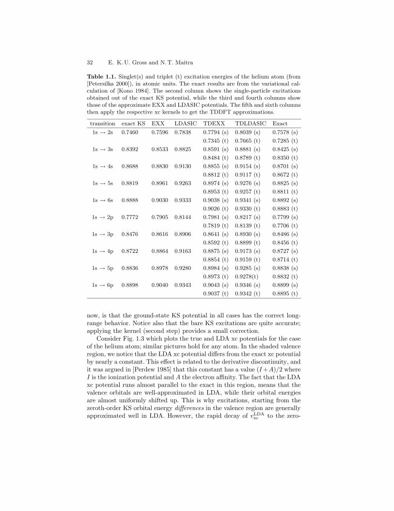
32 E. K. U. Gross and N. T. Maitra
Table 1.1. Singlet(s) and triplet (t) excitation energies of the helium atom (from[Petersilka 2000]), in atomic units. The exact results are from the variational cal-culation of [Kono 1984]. The second column shows the single-particle excitationsobtained out of the exact KS potential, while the third and fourth columns showthose of the approximate EXX and LDASIC potentials. The fifth and sixth columnsthen apply the respective xc kernels to get the TDDFT approximations.
transition exact KS EXX LDASIC TDEXX TDLDASIC Exact
1s → 2s 0.7460 0.7596 0.7838 0.7794 (s) 0.8039 (s) 0.7578 (s)
0.7345 (t) 0.7665 (t) 0.7285 (t)
1s → 3s 0.8392 0.8533 0.8825 0.8591 (s) 0.8881 (s) 0.8425 (s)
0.8484 (t) 0.8789 (t) 0.8350 (t)
1s → 4s 0.8688 0.8830 0.9130 0.8855 (s) 0.9154 (s) 0.8701 (s)
0.8812 (t) 0.9117 (t) 0.8672 (t)
1s → 5s 0.8819 0.8961 0.9263 0.8974 (s) 0.9276 (s) 0.8825 (s)
0.8953 (t) 0.9257 (t) 0.8811 (t)
1s → 6s 0.8888 0.9030 0.9333 0.9038 (s) 0.9341 (s) 0.8892 (s)
0.9026 (t) 0.9330 (t) 0.8883 (t)
1s → 2p 0.7772 0.7905 0.8144 0.7981 (s) 0.8217 (s) 0.7799 (s)
0.7819 (t) 0.8139 (t) 0.7706 (t)
1s → 3p 0.8476 0.8616 0.8906 0.8641 (s) 0.8930 (s) 0.8486 (s)
0.8592 (t) 0.8899 (t) 0.8456 (t)
1s → 4p 0.8722 0.8864 0.9163 0.8875 (s) 0.9173 (s) 0.8727 (s)
0.8854 (t) 0.9159 (t) 0.8714 (t)
1s → 5p 0.8836 0.8978 0.9280 0.8984 (s) 0.9285 (s) 0.8838 (s)
0.8973 (t) 0.9278(t) 0.8832 (t)
1s → 6p 0.8898 0.9040 0.9343 0.9043 (s) 0.9346 (s) 0.8899 (s)
0.9037 (t) 0.9342 (t) 0.8895 (t)
now, is that the ground-state KS potential in all cases has the correct long-range behavior. Notice also that the bare KS excitations are quite accurate;applying the kernel (second step) provides a small correction.
Consider Fig. 1.3 which plots the true and LDA xc potentials for the caseof the helium atom; similar pictures hold for any atom. In the shaded valenceregion, we notice that the LDA xc potential differs from the exact xc potentialby nearly a constant. This effect is related to the derivative discontinuity, andit was argued in [Perdew 1985] that this constant has a value (I +A)/2 whereI is the ionization potential and A the electron affinity. The fact that the LDAxc potential runs almost parallel to the exact in this region, means that thevalence orbitals are well-approximated in LDA, while their orbital energiesare almost uniformly shifted up. This is why excitations, starting from thezeroth-order KS orbital energy differences in the valence region are generallyapproximated well in LDA. However, the rapid decay of vLDA
xc to the zero-

1 Introduction to TDDFT 33
r
KS
pote
ntia
l
(LDA − exact) potential
exact, has Coulombic decayLDA, has exponential decay
−3
−2.5
−2
−1.5
−1
−0.5
1 2 3 4 5 6 7 8
0.5
1
8 0
Fig. 1.3. The exact and LDA KS potentials for the He atom.
asymptote means that the higher-excitation energies are underestimated andeventually get squeezed into the continuum. (Unfortunately for the case ofthe He atom, this happens to even the lowest excitations).
The top panel of Fig. 1.4 illustrates two effects of the too rapid decay ofthe LDA potential on the optical spectrum: (i) it pushes the valence levels up,so that the ionization potential is too low; the onset of the LDA continuumis red-shifted compared to the exact, and (ii) there is no Rydberg seriesin the LDA spectrum; instead their oscillator strengths appear in the LDAcontinuum, but in fact are not badly approximated [Wasserman 2003]. Thereason for this accuracy is due to the LDA and true xc potentials runningnearly parallel in the valence region: the LDA HOMO orbital, out of whichthe transitions are computed, very well-approximates the true HOMO, whilethe LDA continuum state at energy E = ω + ILDA follows very closely theexact continuum state at energy E = ω + Iexact until a distance large enoughaway from the nucleus that the integrand does not contribute due to thedecay of the HOMO. Noting that KS spectra are not true spectra, the lowerpanel shows the TDDFT-corrected spectrum using ALDA for the xc kernel;although not resolving the discrete part of the spectra, the overall oscillatorstrength envelope is not bad. For a detailed discussion, we refer the readerto [Wasserman 2003].
The purpose of this case study was to illustrate the workings of TDDFTresponse and investigate only the simplest functional on the simplest system.We note that most molecules have many more lower-lying excited states sothat GGA’s can do a much better job for more excitations. We return to thequestion of functional approximations in later sections throughout this book.
1.6 Higher-order response
Often the simplest way to calculate the non-linear response of a system to anexternal perturbation is via time-propagation. But, like in the linear-response

34 E. K. U. Gross and N. T. Maitra
exact KSLDA
exact calculationsexperiment
LDA/ALDA
ω
optic
al in
tens
ityop
tical
inte
nsity
0
0.5
1
1.5
0.6 0.8 1 1.2 1.4 1.6 1.8
0
0.5
1
1.5
0.6 0.8 1 1.2 1.4 1.6 1.8
Fig. 1.4. Optical absorption spectrum in the He atom (from [Wasserman 2003]).The top panel shows the bare exact KS and LDA KS spectra. The lower panel showsthe TDDFT ALDA spectra (dashed line, from [Stener 2001]), the exact calculationsfrom [Kono 1984] and experimental results from [Samson 1994].
case, it can be instructive to perform the non-linear response calculation di-rectly in frequency-space. The higher-order terms in Eq. (1.46) can be ex-pressed in terms of higher-order density-density response functions:
n2(x) =1
2!
∫
dx′
∫
dx′′ χ(2)(x, x′, x′′)δv(x′)δv(x′′) (1.89a)
n3(x) =1
3!
∫
dx′
∫
dx′′
∫
dx′′′ χ(2)(x, x′, x′′, x′′′)δv(x′)δv(x′′)δv(x′′′)
. . . (1.89b)
where we used the short-hand x = (r, t) and∫
dx =∫
d3r∫
dt . For quadraticresponse, the analogues of Eqs. (1.48) and (1.49) are
χ(2)(x, x′, x′′) =δ2n(x)
δvext(x′)δvext(x′′)
∣
∣
∣
∣
n0
= −∑
P
θ(t− τ)θ(t− τ ′)〈Ψ0|[[nH(x), nH(x′)], nH(x′′)]|Ψ0〉
(1.90)
where the sum goes over all permutations of x, x′, x′′. Clearly, the interactinghigher-order response functions are very difficult to calculate directly andinstead we look to extract them from the KS response functions and xckernels. Manipulations similar to those in the linear response case, but more
1 Introduction to TDDFT 35
complicated, lead to [Gross 1996]:
χ(2)(x, x′, x′′) =
∫
dy
∫
dy′ χ(2)KS(x, y, y′)
δvKS(y)
δv(x′)
∣
∣
∣
∣
n0
δvKS(y′)
δv(x′′)
∣
∣
∣
∣
n0
+
∫
dy χKS(x, y)
∫
dy′
∫
dy′′ kxc[n0](y, y′, y′′)χ(y′, x′)χ(y′′, x′′)
+
∫
dy χKS(x, y)
∫
dy′ fHxc[n0](y, y′)χ(2)(y′, x′, x′′) . (1.91)
Here χ(2)KS = δ2n(x)/δvKS(x′)δvKS(x′′)
∣
∣
n0is the KS second-order density-
response function, and
kxc[n0](rt, r′t′, r′′t′′) =δ2vxc[n](r, t)
δn(r′, t′)δn(r′′, t′′)
∣
∣
∣
∣
n=n0
(1.92)
is the dynamical second-order xc kernel. In the adiabatic approximation,
kadiaxc (r, r′, r′′) =
δ3Exc[n]
δn(r)δn(r′)δn(r′′)(1.93)
with Exc[n] a ground-state xc energy functional. Making Fourier-transformswith respect to t− t′ and t− t′′, we arrive at the Dyson equation
n2(r, ω) =1
2
∫
dω′
∫
d3r1d3r2χ
(2)(r, r1, r2, ω, ω−ω′)δv(r1, ω)δv(r2, ω−ω′)
=1
2
∫
dω′
∫
d3r1d3r2
(
χ(2)KS(r, r1, r2, ω, ω − ω′)δvKS(r1, ω)δvKS(r2, ω − ω′)
+
∫
d3r3χKS(r, r1, ω)kxc(r1, r2, r3, ω, ω − ω′)n1(r2, ω′)n1(r3, ω − ω′)
)
+
∫
d3r1d3r2χKS(r, r1, ω)fHxc(r1, r2, ω)n2(r2, ω) (1.94)
Likewise, one may work out Dyson-like response equations for the higher-order response functions, each time introducing a new xc kernel. These deter-mine the frequency-dependent non-linear response. Sum-over-states expres-sions for the non-interacting density-response functions up to third-order maybe found in [Senatore 1987]. We also point to Chapter II.4, where higher-orderresponse is discussed within a Sternheimer scheme.
[Gross 1996] pointed out a very interesting hierarchical structure that theTDDFT response equations have. At any order i,
ni(ω) = Mi(ω) + χKS(ω) ⋆ fHxc(ω) ⋆ ni(ω) (1.95)
where Mi depends on lower-order density-response (and response-functionsup to ith order). The last term on the right of Eq. (1.95) has the samestructure for all orders. If we define the operator
L(ω) = 1− χKS(ω) ⋆ fHxc(ω) (1.96)
36 E. K. U. Gross and N. T. Maitra
thenL(ω) ⋆ ni(ω) = Mi(ω) (1.97)
so L(ω) plays a significant role in determining what new poles are generatedfrom electron-interaction effects in all orders of response [Elliott 2011].
1.7 Approximate functionals
As noted earlier, the xc potential is a functional of the density, the initial truestate, and the initial KS state. The exact functional has “memory”, that is, itdepends on the history of the density as well as these two initial states. This isdiscussed to some extent in Chapter III.1. In fact these two sources of memoryare intimately related, and often the elusive initial-state dependence can bereplaced by a type of history-dependence. The xc kernel of linear responsehas simpler functional dependence, as it measures xc effects around the initialground-state only. Functionally it depends only on the initial ground-statedensity, while memory-dependence appears as dependence on frequency inthe arguments of fxc.
It should be noted that when running response calculations, for formalconsistency, the same approximation should be used for the xc kernel asis used for the ground-state potential, i.e. there must exist an approximatefunctional vapp
xc [n](r, t) such that the initial potential vappxc [n](r, t = 0) is used
in the KS ground-state calculation, and such that fappxc [n](r, r′, t − t′) =
δvappxc [n](r, t)/δn(r′, t′) is used in the time-dependent response part. If dif-
ferent functionals were used for each step, one has left the framework ofTDDFT response, since the calculation no longer is equivalent to computingthe time-dependent response to an external perturbation. Nevertheless, thisfact is often ignored in practical calculations.
We now will outline some of the different approximations people use today.
1.7.1 Adiabatic approximations: ALDA, AGGA, AB3LYP ...
Almost all functionals in use today have no memory-dependence whatsoever.They are “adiabatic”, meaning that the density at time t is plugged into aground-state functional, i.e.
vadiaxc [n](r, t) = vGS
xc [n(t)](r) . (1.98)
For the xc kernel, we retrieve the static kernel of Eq. (1.80)
fadiaxc [nGS](rt, r′t′) =
δvGSxc [n(t)](r)
δn(r′, t′)
∣
∣
∣
∣
nGS
= δ(t− t′)δ2Exc[n]
δn(r)δn(r′)
∣
∣
∣
∣
nGS
.
(1.99)If the external time-dependence is very slow (adiabatic) and the system be-gins in a ground-state, this approximation is justified. But this is not the

1 Introduction to TDDFT 37
usual case. Even if the density is reproducible by a system in its a ground-state, the wavefunction is usually not, so this appears to be quite a severeapproximation. Nevertheless adiabatic approximations are the workhorse ofthe myriads of applications of TDDFT today, and work pretty well for mostcases (but not all). Why this is so is still somewhat of an open question.Certainly adiabatic approximations trivially satisfy many exact conditionsrelated to memory-dependence, so perhaps this is one reason. This is similarto the justification used for the success of LDA in the ground-state case, andthe subsequent development of generalized gradient approximations (GGA)based on satisfaction of exact conditions. When considering excitation ener-gies of systems, the bare KS orbital energy differences themselves are rea-sonably good approximations to the exact excitation energies. The kernelthen just adds a small correction on top of this good zeroth order estimate,and hence even the simplest approximation such as an adiabatic one does adecent job. Many cases where the usual approximations fail, such as excitedstates of multiple-excitation character, or certain types of electronic quantumcontrol problems, can be clearly understood to arise from lack of memory inthe adiabatic approximation.
The adiabatic local density approximation, or ALDA is the simplest pos-sible approximation in TDDFT. It is also often called TDLDA (for time-dependent LDA):
vALDAxc [n](r, t) = vhom
xc (n(r, t)) =d
dn[nehom
xc (n)]|n=n(r,t) (1.100)
where ehomxc (n)) is the xc energy per particle of the homogeneous electron gas.
The corresponding xc kernel
fALDAxc [nGS](rt, r′t′) = δ(t− t′)δ(r − r′)
d2
dn2[nehom
xc (n)]|n=nGS(r) (1.101)
which is completely local in both space and time, and its Fourier-transform,Eq. (1.86a) is frequency-independent. Although it might appear justified onlyfor slowly-varying systems in space and in time, it often gives reasonable re-sults for systems far from this limit. Adiabatic GGA’s and hybrid functionalsare most commonly used for finite systems; hybrids in particular for thehigher-lying excitations where it is important to catch the tail of the molec-ular potential.
1.7.2 Orbital functionals
A natural way to break free of the difficulties in approximating functionalsof the density alone, and still stay within TDDFT, is to develop functionalsof the KS orbitals. The simplest functional of this kind is the exact-exchange

38 E. K. U. Gross and N. T. Maitra
functional, derived from the action:
Ax[φiα] = −1
2
∑
σ
Nσ∑
i,j
∫ t
−∞
dt′∫
d3r
∫
d3r′
ϕ∗iσ(r′, t′)ϕjσ(r′, t′)ϕiσ(r, t′)ϕ∗
jσ(r, t′)
|r − r′| (1.102)
Note that for more general functionals, the action needs to be defined onthe Keldysh contour [van Leeuwen 1998] (see also Chapter III.5). The exactexchange potential is then given by
vx,σ[φjα](r, t) =δAx[φjα]δnσ(r, t)
(1.103)
Orbital functionals are in fact implicit density functionals because orbitalsare trivially functionals of the single-particle KS potential, which, by the RGtheorem, is a functional of the density, ϕj [vKS[n]](r, t). The xc potential isgiven by the functional derivative of the action with respect to the (spin-)density and the xc kernel is the second functional derivative. The equationsatisfied by the xc potential is usually called the (time-dependent) OptimizedEffective Potential (OEP) equation, and is discussed in Chapter III.5. Theexact-exchange functional is local in time when viewed as a functional of KSorbitals. However, viewed as an implicit functional of the density, it is non-local in time. The second-functional derivative with respect to the densitythen has a non-trivial dependence on t− t′.
Invoking a Slater-type approximation in each functional derivative ofEq. (1.102), [Petersilka 1996a, Petersilka 1998] deduced,
fPGGx σσ′ (r, r′) = −δσσ′
1
|r− r′||∑
k fkσ ϕkσ(r)ϕ∗kσ(r′)
∣
∣
2
nσ(r)nσ(r′). (1.104)
Evidently, with this approximation, the non-trivial (t− t′)-dependence of theexact exchange-only kernel is not accounted for. However, it is clearly spatiallynon-local. For one and two electrons, Eq. (1.104) is exact for exchange.
The full numerical treatment of exact-exchange (TDEXX), including me-mory-dependence, has recently seen some progress. In [Gorling 1997], the ex-act x kernel was derived from perturbation theory along the time-dependentadiabatic connection. One scales the electron-electron interaction by λ, defin-ing a Hamiltonian
Hλ = T + λVee + V λ(t) (1.105)
such that the density nλ(r, t) = n(r, t) for any λ much like as is done inground-state DFT. The initial state Ψλ
0 is chosen to reproduce the same ini-
tial density and its first time-derivative, at any λ. For λ = 0, V λ(t) = VKS(t)

1 Introduction to TDDFT 39
and for λ = 1, V λ(t) = Vext(t). Performing perturbation theory to first or-der in λ yields the TDEXX potential and kernel, found in [Gorling 1997,Gorling 1998a, Gorling 1998b] while higher orders give correlation function-als. Until very recently there was only limited use of this kernel due tonumerical instabilities [Shigeta 2006]. A series of papers reformulated theproblem in terms of response of the KS potential itself, avoiding the cal-culation of numerically prohibitive inverse response functions [Hesselmann2009, Gorling 2010, Ipatov 2010], but needing a time-consuming frequency-iteration for each excitation energy. Most recently, a very efficient methodhas been derived that translates the problem onto a generalized eigenvalueproblem [Hesselmann 2011]. Although the results of full exact-exchange cal-culations for excitation energies are often numerically close to those of time-dependent Hartree-Fock [Hesselmann 2011] in the cases so far studied, thereis a fundamental difference in the two methods: TDEXX operates with a local(multiplicative) potential, while that of time-dependent Hartree-Fock is non-local, i.e. an integral operator. Furthermore, the Hartree-Fock single-particleenergy differences εHF
a −εHFi are usually too large and hence the Hartree-Fock
kernel reduces the Hartree-Fock energy difference, while εKSa − εKS
i withinEXX tend to be too small, so the x-kernel of TDDFT has to increase the KSexcitation energy. Beyond the linear response regime, [Wijewardane 2008]computed nonlinear dynamics in semiconductor wells within TDEXX.
Another class of orbital-dependent functionals are self-interaction-corrected(SIC) functionals. An approximation at a similar level to Eq. (1.104) can befound in [Petersilka 2000].
1.7.3 Hydrodynamically based kernels
The first proposal to incorporate memory-dependence was in [Gross 1985],who suggested to use the frequency-dependent xc kernel of the homogeneouselectron gas in the sense of an LDA:
fLDAxc [n0](r, r′, ω) = fhom
xc (n0(r), |r − r′|, ω) . (1.106)
and furthermore that the response n1(r, ω) is slowly varying enough on thelength-scale of fhom
xc (n0(r), |r − r′|;ω) that only its uniform component con-tributes. That is, taking a spatial Fourier-transform with respect to r − r′,we include only the zeroth-Fourier component. This gives the Gross-Kohnkernel:
fGKxc [n0](r, r′, ω) = δ(r − r′)fhom
xc (n0(r), q = 0, ω) (1.107)
where q is the spatial Fourier transform variable. One requires the knowledgeof the frequency-dependent response of a uniform electron gas, about which,indeed many exact properties are known, and parametrizations, believed tobe accurate, exist [Conti 1999, Conti 1997, Gross 1985, Qian 2002, Qian 2003].Chapter VI.2 discusses some of these.

40 E. K. U. Gross and N. T. Maitra
Although the GK approximation has memory, it is completely local inspace, a property which turns out to violate exact conditions, such as thezero-force rule and translational invariance (see Chapters II.2 and VI.2).Even ALDA does not violate these. To go beyond the adiabatic approx-imation consistently, both spatial and temporal non-locality must be in-cluded. This is perhaps not surprising in view of the fact that the densitythat at time t is at location r was at an earlier time t′ < t at a differ-ent location, i.e. memory is carried along with the fluid element. The de-velopment of memory-dependent functionals, often based on hydrodynamicschemes, is discussed further in Chapter III.1 and Chapter VI.2. These in-clude the Dobson-Bunner-Gross [Dobson 1997], Vignale-Kohn [Vignale 1996],Tokatly [Tokatly 2005a, Tokatly 2005b], and Kurzweil-Baer[Kurzweil 2004]approaches. These are not commonly used; only the Vignale-Kohn functionalhas seen a few applications.
1.8 General performance and challenges
As shown in Sect. 1.2, TDDFT is an exact reformulation of non-relativisitictime-dependent quantum mechanics. In principle, it yields exact electronicdynamics and spectra. In practice, its accuracy is limited by the functionalapproximations used. The simplest and computationally most efficient func-tional, ALDA, is local in both space and time, and it is perhaps surprisingthat it works as well as it does. We now discuss cases where it is essentialto go beyond this simple approximation, and, further, beyond its adiabaticcousins. We organize this section into three parts: linear response in extendedsystems, linear response in finite systems, and real-time dynamics beyond theperturbative regime.
1.8.1 Extended systems
We first ask, how well does ALDA perform for the response of solids? In simplemetals, ALDA does well, and captures accurately the plasmon dispersioncurves [Quong 1993]. In fact, the ordinary plasmon is captured reasonablyeven by the Hartree potential alone, i.e. setting fxc = 0, which is calledthe RPA. Applying fALDA
xc improves the description of its dispersion andlinewidth.
The answer to the question above is rather more subtle for non-metallicsystems. ALDA does a good job for electron energy loss (EEL) spectra, bothwhen the impinging electron transfers finite momentum q and in the case ofvanishing momentum-transfer. The EEL spectrum measures the imaginarypart of the inverse dielectric function (see Chapter I.3), which, in terms ofthe density-response function, is given in Eq. 3.54b [Onida 2002, Botti 2007].The optical response, which measures the imaginary part of the macro-scopic dielectric function (see Chapter I.3) is also quite well predicted byALDA [Weissker 2006] for finite wavevector q.

1 Introduction to TDDFT 41
However, for optical response in the limit of vanishing wavevector, q → 0,ALDA performs poorly for non-metallic systems. There are two main prob-lems: (i) The onset of continuous absorption is typically underestimated,sometimes by as much as 30-50%. This problem is due to the fact that theKS gap in LDA is much smaller than the true gap. But even with the exactground-state potential, there is very strong evidence [Knorr 1992, Gruning2006, Niquet 2004] that the exact KS gap is typically smaller than the truegap. To open the gap, the xc kernel must have an imaginary part [Giuliani2005]. This follows from the fundamental Dyson equation (1.59)2: We knowthat the imaginary part of χKS(r, r′, ω) = 0 for ω inside the KS gap. Then,for an approximate fxc(r, r′, ω) that is real, taking the imaginary part ofEq. (1.59) for ω inside the KS gap (0 < ω < EKS
g ), yields
Im χKS(ω) = 0 −→[
1−Re χKS(ω) ⋆ fHxc(ω)]
⋆ Im χ(ω) = 0 . (1.108)
Following the analogous procedure for ω inside the true gap (0 < ω < Eg) ,where Im χ(r, r′ω) = 0, yields
Im χ(ω) = 0 −→ Im χKS(ω) ⋆[
1 + fHxc(ω) ⋆ Re χ(ω)]
= 0 . (1.109)
In view of the fact that fHxc = χ−1KS − χ−1, the expressions inside the square
brackets in (1.108) and (1.109) cannot vanish identically in the full interval0 < ω < EKS
g and 0 < ω < Eg , respectively. (The expressions may vanish atisolated frequencies corresponding to collective excitations). Hence we mustconclude that wherever Im χKS(ω) = 0, then also Im χ(ω) = 0. That is, forfrequencies inside the KS gap, the true response is also zero. Likewise, wher-ever Im χ(ω) = 0, then also Im χKS(ω) = 0. That is, for frequencies insidethe true gap, the KS response is also zero. Putting the two together impliesthat the KS system and the true system must have the same gap when anapproximation for fHxc is used that is purely real. This is clearly a contra-diction, implying that fHxc must have a non-vanishing imaginary part. This,on the other hand, is equivalent to fxc having a frequency-dependence, asmentioned in Sect. 1.5.3. Any adiabatic approximation however takes a ker-nel that is the second density-functional-derivative of a ground-state energyfunctional, and therefore is purely real. Further, as we shall shortly discuss,the kernel must have have a long-ranged part, that goes as 1/q2 as q → 0,to get any non-vanishing correction on the gap. ALDA, on the other hand,is local in space, and so constant in q.
(ii) The second main problem is that ALDA cannot yield any excitonicstructure; again, one needs a long-ranged 1/q2 part in the kernel to get anysignificant improvement on RPA for optical response. To reproduce excitons,an imaginary part to fxc is not required [Reining 2002].
Fundamentally, the long-ranged behaviour of fxc can be deduced fromexact conditions satisfied by the xc kernel, such as the zero-force theorem,
2 This argument is due largely to Giovanni Vignale

42 E. K. U. Gross and N. T. Maitra
that inextricably link time-nonlocality and space-non-locality. This is shownexplicitly in Chapter VI.2. Lack of a long-ranged term in ALDA or AGGAfor finite systems, or for EELs spectra, is not as critical as for the case ofextended systems, since its contribution is much smaller there.
The need for this long-ranged behavior in the xc kernel is, interestingly,not a consequence of the long-rangedness of the Coulomb interaction. A sim-ple way to see this is to consider the SPA Eq. (1.63) for a system of size L3,where, for the extended system we consider L → ∞. The transition densi-ties Φq scale as 1/L3, so for a finite-ranged xc kernel, the xc-correction tothe RPA value scales as 1/L3, and so vanishes in the extended-system limit[Giuliani 2005].
An alternate way of seeing the need for the long-ranged kernel, is to notethat the optical absorption measures the imaginary part of the macroscopicdielectric function, which can be written in terms of a modified density-response function [Botti 2007](and see Eqs. (3.52b) and (3.54) in Chapter I.3.Now χKS(q → 0) ∼ q2 for infinite systems, so if fxc is to have any significantnon-vanishing effect on the optical response, it must have a component thatdiverges as 1/q2 as q → 0.
Recent years have seen a tremendous effort to confront the problem ofoptical response in solids by including spatially-non-local dependence. Exact-exchange was shown in [Kim 2002a] to have apparent success in capturingthe exciton. However, it was shown later in [Bruneval 2006] that if done care-fully, the excitonic structure predicted by exact-exchange is far too strong,essentially collapsing the entire spectrum onto the exciton. The earlier cal-culation of [Kim 2002a] fortuitously induced an effective screening of theinteraction, since the long wavelength contributions were cut off in those cal-culations. TDCDFT has also been used [de Boeij 2001], with the motivationthat local functionals of the current-density contain non-local informationof the density, and this is discussed further in Chapter VI.2. Perhaps themost intense progress has been made in the development of kernels derivedfrom many-body perturbation theory (MBPT), leading to what is now knownas the “nanoquanta kernel”. The latter is deduced from the Bethe-Salpeterapproach of MBPT [Bruneval 2005b, Reining 2002, Sottile 2003, Adragna2003, Marini 2003b, Stubner 2004, von Barth 2005]. An important aspect isthat the reference systems in the Bethe-Salpeter approach and the TDDFTapproach are completely different: KS excitation energies and orbitals of thelatter are not quasiparticle energies and wavefunctions that the former buildson. From the point of view of MBPT, the TDDFT xc kernel may be inter-preted as having two roles: shifting the KS excitations to the quasiparticle
ones (so-called f(1)xc ), and then accounting for the electron-hole interaction
(so-called f(2)xc ). In practical uses of the nanoquanta kernel, explicit models
for f(2)xc are used on top of simply the quasiparticle energies (usually in GW
approximation). We refer the reader to [Botti 2007, Onida 2002].

1 Introduction to TDDFT 43
1.8.2 Finite systems
In linear response calculations of optical spectra, use of local or semi-localfunctionals for low-lying excitations, or hybrid functionals for higher-lyingones, within the adiabatic approximation for the xc kernel yields results thatare typically considerably better than those from TDHF or configurationinteraction singles (CIS). These methods scale comparably to TDDFT, whilethe accuracy of TDDFT is, in most cases, far superior.
Most quantum chemistry applications use the B3LYP hybrid functional [Becke1993a, Becke 1993b]. While excitation energies are typically good to withina few tenths of an eV, structural properties fare much better [Furche 2002a,Elliott 2009]. For example, bond-lengths of excited states are within 1%,dipole moments and vibrational frequencies to within 5%. Chapter IV.3 dis-cusses this more. Often the level of accuracy has been particularly useful in ex-plaining, for the first time, mechanisms of processes in biologically and chem-ically relevant systems, e.g. the dual fluorescence in dimethyl-amino-benzo-nitrile [Rappoport 2004], and chiral identification of fullerenes[Furche 2002b].
In the following, we discuss several cases where the simplest approxima-tions like ALDA and AGGA, perform poorly.
To be able to describe Rydberg excitations, it is essential that the ground-state potential out of which the bare KS excitations are computed has thecorrect −1/r asymptotics. LDA and GGA do not have this feature, and aswe have seen already in our case study of the He atom, the Rydberg excita-tions were absent in LDA/GGA. Solutions include exact-exchange methods,self-interaction corrected functionals, and hybrids. Step-like features in theground-state potential as well as spatial non-locality in the xc kernel canalso be essential: a well-known case is in the computation of polarizabilitiesof long-chain molecules [van Faassen 2002, van Gisbergen 1999b, Gritsenko2000], and exact-exchange, as well as TDCDFT-methods have been exploredfor this problem. A more challenging problem is that of molecular dissoci-ation: it is notoriously difficult to obtain accurate ground-state dissociationcurves, since self-interaction errors in the usual functionals leads to fractionalcharges at large separation. As it dissociates, the exact ground-state potentialfor a molecule composed of open-shell fragments such as LiH, develops stepand peak features in the bond-midpoint region [Perdew 1985, Gritsenko 1996,Helbig 2009, Tempel 2009], missed in GGAs and hybrids alike, but crucial fora correct description. To get even qualitatively correct excited state surfaces,frequency-dependence is crucial in the xc kernel [Maitra 2005b, Maitra 2006a](see also Chapter III.1). The essential problem is that the true wavefunc-tion has wandered far from a single-Slater-determinant, making the workof the ground-state exchange-correlation potential and the kernel very dif-ficult. Such cases of strong correlation are one of the major motivators oftime-dependent density-matrix functional theory, discussed in Chapter VI.4.
Another case where frequency-dependence is essential are states of double-excitation character. We will defer a discussion of this to Chapter III.1.

44 E. K. U. Gross and N. T. Maitra
A notorious failure of the usual approximations for finite systems is forcharge-transfer excitations at large-separation [Dreuw 2003, Dreuw 2004,Tozer 2003]. To leading order in 1/R, the exact answer for the lowest charge-transfer excitation frequency is:
ωexactCT → ID −AA − 1/R (1.110)
where ID is the ionization energy of the donor, AA is the electron affin-ity of the acceptor and −1/R is the first electrostatic correction betweenthe now charged species. Charge-transfer excitations calculated by TDDFTwith the usual approximations however severely underestimate Eq. (1.110).Due to the exponentially small overlap between orbitals on the donor andacceptor, located at different ends of the molecule, fxc must diverge expo-nentially with their separation in order to give any correction to the bareKS orbital energy difference [see e.g. Eq. (1.63)]. Semilocal functional ap-proximations for fHxc give no correction, so their prediction for charge-transfer excitations reduces to the KS orbital energy difference, εa − εi =εL(acceptor) − εH(donor), where L,H subscripts indicate the KS LUMOand HOMO, respectively. This is a severe underestimate to the true energy,because the ionization potential is typically underestimated by the HOMOof the donor, due to the lack of the −1/r asymptotics (Sect. 1.5.5), whilethe LUMO of the acceptor lacks the discontinuity contribution to the affin-ity. The last few years have seen many methods to correct the underes-timation of CT excitations, e.g. [Autschbach 2009, Tawada 2004, Vydrov2006b, Zhao 2006, Stein 2009, Hesselmann 2009, Rohrdanz 2009]; most mod-ify the ground-state functional to correct the approximate KS HOMO’s un-derestimation of I, and mix in some degree of Hartree-Fock, and most,but not all [Stein 2009, Hesselmann 2009] determine this mixing via atleast one empirical parameter. Fundamentally, staying within pure DFT,both the discontinuity contribution to A and the −1/R tail in Eq. (1.110)come from fHxc, which must exponentially diverge with fragment separa-tion [Gritsenko 2004]. Worse still, in the case of open-shell fragments, not
covered by most of the recent fixes, additionally the exact fxc is stronglyfrequency-dependent [Maitra 2005b].
We briefly mention two other challenges, which are further discussed laterin this book. The difficulty that usual functionals have in capturing poten-tial energy surfaces near a conical intersection is discussed in Chapter IV.1.This poses a challenge for coupled electron-dynamics using TDDFT, giventhat conical intersections are a critical feature on the potential energy land-scape, funneling nuclear wavepackets between surfaces. The second challengeis the Coulomb blockade phenomenon in calculations of molecular transport.The critical need for functionals with a derivative discontinuity to describethis effect, and to obtain accurate conductances in nanostructures, is furtherdiscussed in Chapter IV.4.

1 Introduction to TDDFT 45
1.8.3 Non-perturbative electron dynamics
In Chapter IV.5 of this book, we shall come back to the fascinating world ofstrong-field phenomena, several of which the usual approximations of TDDFThave had success in describing, and some of which the usual approximationsdo not capture well. Developments in attosecond laser science have openedup the possibility of electronic quantum control; recently the equations forquantum optimal control theory within the TDKS framework have been es-tablished and this is described in Chapter IV.7. Chapters IV.1 and IV.2discuss the difficult but extremely important question of coupling electronsdescribed via TDDFT to nuclear motion described classically, in schemessuch as Ehrenfest dynamics and surface-hopping. Here instead we discuss ingeneral terms the challenges approximations in TDDFT face for real-timedynamics.
However first, we show how useful a density-functional picture of elec-tron dynamics can be for a wide range of processes and questions, via thetime-dependent electron localization function (TDELF). With the adventof attosecond lasers, comes the possibility of probing detailed mechanisms ofelectronic excitations and dynamics in a given process. For example, in chem-ical reactions, can we obtain a picture of bond-breaking and bond-forming?In [Burnus 2005] it was shown how to generalize the definition of the elec-tron localization function (ELF) used to analyze bonding in ground-statesystems [Becke 1990], to time-dependent processes:
TDELF(r, t) =1
1 + [Dσ(r, t)/D0σ(r, t)]
2 , (1.111)
with
Dσ(r, t) = τσ(r, t)− 1
4
|∇nσ(r, t)|2nσ(r, t)
− j2σ(r, t)
nσ(r, t)(1.112)
where jσ is the magnitude of the KS current-density of spin σ, and τσ(r, t) =∑Nσ
i=1 |∇ϕiσ(r, t)|2 is the KS kinetic energy-density of spin σ. In Eq. (1.111),
D0σ(r, t) = τhom
σ (nσ(r, t)) = 35 (6π2)2/3n
5/3σ is the kinetic energy-density of the
uniform electron gas. Using ALDA to evaluate the TDELF, this function hasbeen useful for understanding time-resolved dynamics of chemical bonds inscattering and excitation processes [Burnus 2005, Castro 2007]; features suchas the temporal order of processes, and their time scales are revealed. As anexample, in Fig. 1.5 we reproduce snapshots of the TDELF for laser-inducedexcitation of the π → π∗ transition in the acetylene molecule, studied in[Burnus 2005]. Many interesting features can be observed from the TDELF.As the intensity of the laser field increases, the system begins to oscillate, andionization is visible in the time slices at 1.2111 fs and 1.5692 fs. The figureclearly shows that after 3.5 fs, the transition from the ground-state to theantibonding state is complete: the original single torus signifying the triplebond in the ground-state has split into two separate tori, each around onecarbon atom.

46 E. K. U. Gross and N. T. Maitra
Fig. 1.5. Snapshots of the TDELF for the excitation of acetylene by a 17.5 eVlaser pulse (from [Burnus 2005]), polarized along the molecular axis. The pulse hada total length of 7 fs, an intensity of 1.2 ×10¹⁴ W/cm2.
General success for dynamics in strong fields has been slower than forlinear response applications. There are three main reasons. First, many ofthe observables of interest are not simply related to the time-dependent one-body density, so that, in addition to the approximation for the xc functional,a new ingredient is needed: approximate “observable functionals” to extractthe properties of interest from the KS system. Sometimes these are simplythe usual quantum mechanical operators acting directly on the KS system,e.g. high-harmonic generation spectra are measured by the dipole momentof the system,
∫
d3r n(r, ω)z. But if the observable is not simply related tothe density, such as ionization probabilities [Ullrich 1997, Petersilka 1999], orcross-sections in atomic collisions [Henkel 2009], in principle an observablefunctional is needed. Simply extracting double-ionization probabilities andmomentum-densities from the KS system typically fails [Lappas 1998, Wilken2006, Wilken 2007, Rajam 2009].
Second, lack of memory dependence in the usual xc approximations hasbeen suggested to be often far more problematic than in the linear-responseregime as is discussed in Chapter III.1. We must deal with the full xc poten-tial vxc[n;Ψ0, Φ0](r, t), instead of the simpler xc kernel. The exact functionaldepends on the history of the density as well as on the initial state but almostall functionals used today are adiabatic. Third, a particularly severe difficultyis encountered when a system starting in a wavefunction dominated by a sin-gle Slater determinant (SSD) evolves to a state that fundamentally needsat least two SSDs to describe it. This is the time-dependent (TD) analogof ground-state static correlation, and arises in electronic quantum controlproblems [Maitra 2002b, Burke 2005a], in ionization [Rajam 2009], and incoupled electron-ion dynamics [Levine 2006]. The TD KS system evolves the
1 Introduction to TDDFT 47
occupied orbitals under a one-body Hamiltonian, remaining in an SSD: theKS one-body density matrix is always idempotent (even with exact function-als), while, in contrast, that of the true system develops eigenvalues (naturaloccupation numbers) far from zero or one in these applications [Appel 2010].The exact xc potential and observable functionals consequently develop com-plicated structure that is difficult to capture in approximations. For example,in [Rajam 2009], a simple model of ionization in two-electron systems showedthat the momentum distribution computed directly from the exact KS sys-tem contains spurious oscillations due to using a single, necessarily delocal-ized orbital, a non-classical description of the essentially classical two-electrondynamics.

48 E. K. U. Gross and N. T. Maitra
References
Adragna, G., R. del Sole, and A. Marini, 2003, “Ab initio calculation of theexchange-correlation kernel in extended systems”, Phys. Rev. B, vol. 68, pp.165108-1–5.
Ando, T., 1977a, “Inter-subband optical-absorption in space-charge layers on semi-conductor surfaces”, Z. Phys. B, vol. 26, pp. 263–272.
Ando, T., 1977b, “Inter-subband optical transitions in a surface space-charge layer”,Solid State Commun., vol. 21, pp. 133–136.
Appel, H., E. K. U. Gross, and K. Burke, 2003, “Excitations in Time-DependentDensity-Functional Theory”, Phys. Rev. Lett., vol. 90, pp. 043005-1–4.
H. Appel and M. Di Ventra, 2009, “Stochastic quantum molecular dynamics”, Phys.Rev. B, vol. 80, pp. 212303-1-4.
Appel, H. and E. K. U. Gross, 2010, “Time-dependent natural orbitals and occupa-tion numbers”, Europhys. Lett. vol. 92, pp. 23001-1–5.
Autschbach, J., 2009, “Highlight article: Charge-transfer excitations and time-dependent density functional theory: Problems and some proposed solutions”,ChemPhysChem, vol. 10, pp. 1757–1760.
Baer, R., and N. Siam, 2004, “Real-time study of the adiabatic energy loss in anatomic collision with a metal cluster”, J. Chem. Phys. vol. 121, pp. 6341–6346.
Bartolotti, L. J., 1981, “Time-dependent extension of the Hohenberg-Kohn-Levyenergy-density functional”, Phys. Rev. A, vol. 24, pp. 1661–1667.
Bartolotti, L. J., 1982, “Time-dependent Kohn-Sham density-functional theory”,Phys. Rev. A, vol. 26, pp. 2243–2244.
Bartolotti, L. J., 1984, “Variation-perturbation theory within a time-dependentKohn Sham formalism: An application to the determination of multipole po-larizabilities, spectral sums, and dispersion coefficients”, J. Chem. Phys., vol.80, pp. 5687–5695.
Bartolotti, L. J., 1987, “Velocity form of the Kohn-Sham frequency-dependent po-larizability equations”, Phys. Rev. A, vol. 36, pp. 4492–4493.
Bauernschmitt, R., and R. Ahlrichs, 1996a, “Treatment of electronic excitationswithin the adiabatic approximation of time dependent density functional the-ory”, Chem. Phys. Lett, vol. 256, pp. 454–464.
Becke, A. D., and K. E. Edgecombe, 1990, “A simple measure of electron localizationin atomic and molecular systems”, J. Chem. Phys., vol. 92 pp. 5397–5403.
Becke, A.D., 1993a, “A new mixing of Hartree-Fock and local density-functionaltheories”, J. Chem. Phys., vol. 98, pp. 1372–1377.
Becke, A. D., 1993b, “Density-functional thermochemistry. III. The role of exactexchange”, J. Chem. Phys., vol. 98, pp. 5648–5652.
Bloch, F., 1933, “Bremsvermogen von Atomen mit mehreren Electronen”, Z. Phys.,vol. 81, pp. 363–376.
Botti, S., A. Schindlmayr, R. Del Sole, and L. Reining, 2007, “Time-dependentdensity-functional theory for extended systems”, Rep. Progr. Phys., vol. 70,pp. 357–407.
Bruneval, F., F. Sottile, V. Olevano, R. Del Sole and L. Reining, 2005b, “Many-Body Perturbation Theory Using the Density-Functional Concept: Beyondthe GW Approximation”, Phys. Rev. Lett., vol. 94, pp. 186402-1–4.
Bruneval, F., F. Sottile, V. Olevano and L. Reining, 2006, “Beyond time-dependentexact exchange: The need for long-range correlation”, J. Chem. Phys, vol. 124,pp. 144113-1–9.

1 Introduction to TDDFT 49
Burke, K., J. Werschnik, and E. K. U. Gross, 2005a, “Time-dependent density func-tional theory: Past, present, and future”, J. Chem. Phys. vol. 123, pp. 062206-1–9.
Burke, K., R. Car, and R. Gebauer, 2005c, “Density-Functional Theory of theElectrical Conductivity of Molecular Devices”, Phys. Rev. Lett., vol. 94, pp.146803-1-4.
Burnus, T., M. A. L. Marques, and E. K. U. Gross, 2005, “Time-dependent electronlocalization function”, Phys. Rev. A, vol. 71, pp. 010501-1–4(R).
Caillat, J., J. Zanghellini, M. Kitzler, O. Koch, W. Kreuzer, and A. Scrinzi, 2005,“Correlated multielectron systems in strong laser fields - an mctdhf approach”,Phys. Rev. A, vol. 71 pp. 012712-1–13.
Casida, M. E., 1995, “Time-dependent density functional response theory formolecules”, in Recent Advances in Density Functional Methods, edited by D. E.Chong, vol. 1 of Recent Advances in Computational Chemistry, pp. 155–192(World Scientific, Singapore).
Casida, M. E., 1996, “Time-dependent density functional response theory of molec-ular systems: Theory, computational methods, and functionals”, in RecentDevelopments and Application of Modern Density Functional Theory, editedby J. M. Seminario, pp. 391–439 (Elsevier, Amsterdam).
Casida, M. E., F. Gutierrez, J. Guan, F.-X. Gadea, D. R. Salahub, and J.-P. Daudey,2000, “Charge-transfer correction for improved time-dependent local densityapproximation excited-state potential energy curves: Analysis within the two-level model with illustration for H2 and LiH”, J. Chem. Phys., vol. 113, pp.7062–7071.
Castro, A., T. Burnus, M. A. L. Marques, E. K. U. Gross, 2007, “Time-dependentelectron localization function: A tool to visualize and analyze ultrafast pro-cesses”, in Analysis and Control of Ultrafast Photoinduced Reactions, SpringerSeries in Chemical Physics, vol. 87, pp. 553–574.
X. Zheng, F. Wang, C. Y. Yam, Y. Mo and G. Chen, 2007, “Time-dependentdensity-functional theory for open systems”, Phys. Rev. B, vol. 75, pp. 195127.
Conti, S., R. Nifosı, and M. P. Tosi, 1997, “The exchange - correlation potential forcurrent-density functional theory of frequency-dependent linear response”, J.Phys. Condens. Matter, vol. 9, pp. L475–L482.
Conti, S., and G. Vignale, 1999, “Elasticity of an electron liquid”, Phys. Rev. B,vol. 60, pp. 7966–7980.
D’Agosta, R., and G. Vignale, 2005a, “Non-V-representability of currents in time-dependent many particle systems”, Phys.Rev.B, vol. 71, pp. 245103-1–6.
D’Agosta, R., and G. Vignale, 2006, “Relaxation in Time-Dependent Current-Density-Functional Theory”, Phys. Rev. Lett., vol. 96, pp. 016405-1–4.
d’Amico, I., and C.A. Ullrich, 2006, “Dissipation through spin Coulomb drag inelectronic spin transport and optical excitations”, Phys. Rev. B., vol. 74, pp.121303-1–4.
d’Amico, I. and C.A. Ullrich, 2010, “Coulomb interactions and spin transport insemiconductors: The spin Coulomb drag effect”, Physica Status Solidi (b), vol.247, pp. 235-247.
de Boeij, P. L., F. Kootstra, J. A. Berger, R. van Leeuwen, and J. G. Snijders, 2001,“Current density functional theory for optical spectra: A polarization func-tional”, J. Chem. Phys., vol. 115, pp. 1995–1999.

50 E. K. U. Gross and N. T. Maitra
Deb, B. M., and S.K. Ghosh, 1982, “Schrodinger fluid dynamics of many-electronsystems in a time-dependent density-functional framework”, J. Chem. Phys.,vol. 77, pp. 342–348.
Dhara, A. K., and S. K. Ghosh, 1987, “Density-functional theory for time-dependentsystems”, Phys. Rev. A, vol. 35, pp. 442–444.
Di Ventra, M., and R. D’Agosta, 2007, “Stochastic Time-Dependent Current-Density-Functional Theory”, Phys. Rev. Lett., vol. 98, pp. 226403-1–4.
Dobson, J. F., M. Bunner, and E. K. U. Gross, 1997, “Time-Dependent DensityFunctional Theory beyond Linear Response: An Exchange-Correlation Poten-tial with Memory”, Phys. Rev. Lett., vol. 79, pp. 1905–1908.
Dreizler, R. M., and E. K. U. Gross, 1990, Density Functional Theory: An Approachto the Quantum Many-Body Problem (Springer, Berlin).
Dreuw, A., J. L. Weisman, and M. Head-Gordon, 2003, “Long-range charge-transferexcited states in time-dependent density functional theory require non-localexchange”, J. Chem. Phys., vol. 119, pp. 2943–2946.
Dreuw, A., and M. Head-Gordon, 2004, “Failure of Time-Dependent Den-sity Functional Theory for Long-Range Charge-Transfer Excited States:The Zincbacteriochlorin-Bacteriochlorin and Bacteriochlorophyll-SpheroideneComplexes”, J. Am. Chem. Soc., vol. 126, pp. 4007–4016.
Elliott, P., F. Furche, and K. Burke, 2009, “Excited states from time-dependentdensity functional theory”, in Reviews in Computational Chemistry, edited byK. B. Lipkowitz and T. R. Cundari, pp. 91–165 (Wiley, Hoboken, NJ)
Elliott, P., S. Goldson, C. Canahui, N. T. Maitra, 2011, “Perspectives ondouble-excitations in TDDFT”, Chem. Phys., in press. Available online athttp://dx.doi.org/10.1016/j.chemphys.2011.03.020.
Errea, L.F., L. Mendez, A. Riera, M. Yanez, J. Hanssen, C. Harel, and A. Salin,1985, “The LiH2+ quasimolecule: A comparison between the configurationinteraction and the OEDM approaches”, J. Physique vol. 46, pp. 709.
Fetter, A. L., and J. D. Walecka, 1971, Quantum Theory of Many-Particle Systems(McGraw-Hill, New York).
Furche, F., and R. Ahlrichs, 2002a, “Adiabatic time-dependent density functionalmethods for excited state properties”, J. Chem. Phys., vol. 117, pp. 7433–7447;ibid, vol. 121, p. 12772 (E) (2004).
Furche, F., and R. Ahlrichs, 2002b, “Absolute Configuration of D2-SymmetricFullerene C84”, J. Am. Chem. Soc., vol. 124, pp. 3804–3805.
Gavnholt, J., A. Rubio, T. Olsen, K. S. Thygesen, and J. Schi/otz, 2009, “Hot-electron-assisted femtochemistry at surfaces: A time-dependent density func-tional theory approach”, Phys. Rev. B, vol. 79, pp. 195405.
Gebauer, R., and R. Car, 2004a, “Current in Open Quantum Systems”, Phys. Rev.Lett., vol. 93, pp. 160404-1–4.
Ghosh, S. K., and B M. Deb, 1982, “Schrodinger fluid dynamics of many electronsystems in a time-dependent density-functional framework”, J. Chem. Phys.vol. 77, pp. 342.
Ghosh, S. K., and B. M. Deb, 1983a, “A density-functional calculation of dynamicdipole polarizabilities of noble gas atoms”, Theor. Chim. Acta vol. 62, pp. 209.
Ghosh, S. K., and B. . Deb, 1983b, “A simple density-functional calculation offrequency-dependent multipole polarizabilities of noble gas atoms” J. Mol.Struct.: THEOCHEM vol. 103, pp. 163.

1 Introduction to TDDFT 51
Ghosh, S. K., and A. K. Dhara, 1988, “Density-functional theory of many-electronsystems subjected to time-dependent electric and magnetic fields”, Phys. Rev.A, vol. 38, pp. 1149–1158.
Giuliani, G. F., and G. Vignale, 2005, Quantum Theory of the Electron Liquid (Cam-bridge University Press).
A. Gorling, 1997, “Time-dependent Kohn-Sham formalism”, Phys. Rev. A., vol. 55,pp. 2630-2639.
Gorling, A., 1998a, “Exact exchange-correlation kernel for dynamic response prop-erties and excitation energies in density-functional theory”, Phys. Rev. A, vol.57, pp. 3433–3436.
Gorling, A., 1998b, “Exact exchange kernel for time-dependent density-functionaltheory”, Int. J. Quantum Chem., vol. 69, pp. 265–277.
Gorling, A., A. Ipatov, W. Gotz, and A. Hesselmann, 2010, “Density-FunctionalTheory with Orbital-Dependent Functionals: Exact-Exchange Kohn-Shamand Density-Functional Response Methods”, Z. Phys. Chem. vol. 224, pp.325
Grabo, T., M. Petersilka, and E. K. U. Gross, 2000b, “Molecular excitation en-ergies from time-dependent density functional theory”, J. Mol. Struct.:THEOCHEM vol. 501–502, 353–367.
Gritsenko, O. V., and E. J. Baerends, 19967, “Effect of molecular dissociation onthe exchange-correlation Kohn-Sham potential”, Phys. Rev. A, vol. 54, pp.1957–1972.
Gritsenko, O. V., S. J. A. van Gisbergen, P. R.T. Schipper, and E. J. Baerends,2000, “Origin of the field-counteracting term of the Kohn-Sham exchange-correlation potential of molecular chains in an electric field”, Phys. Rev. A,vol. 62, pp. 012507-1–10.
Gritsenko, O. V., and E. J. Baerends, 2004, “Asymptotic correction of the exchange–correlation kernel of time-dependent density functional theory for long-rangecharge-transfer excitations”, J. Chem. Phys. vol. 121, pp. 655.
Gross, E. K. U., and W. Kohn, 1985, “Local density-functional theory of frequency-dependent linear response”, Phys. Rev. Lett., vol. 55, pp. 2850–2852; ibid, vol.57, p. 923(E) (1986).
Gross, E. K. U., D. Mearns, L. N. Oliveira, 1988, “Zeros of the frequency-dependentlinear density response”, Phys. Rev. Lett., vol. 61, p. 1518.
Gross, E. K. U., and W. Kohn, 1990, “Time-Dependent Density Functional Theory”,Adv. Quant. Chem., vol. 21, pp. 255–291.
Gross, E. K. U., J. Dobson, and M. Petersilka, 1996, “Density functional theory oftime-dependent phenomena”, in Density Functional Theory II, edited by R.F.Nalewajski, vol. 181 of Topics in Current Chemistry, pp. 81–172 (Springer,Berlin).
Gruning, M., A. Marini, and A. Rubio, 2006, “Density functionals from many-body perturbation theory: The band gap for semiconductors and insulators”,J. Chem. Phys., vol. 124, pp. 154108–154117.
Harriman, J. E., 1981, “Orthonormal orbitals for the representation of an arbitrarydensity”, Phys. Rev. A, vol. 24, pp. 680–682.
Hatcher, R., M. Beck, A. Tackett, and S. T. Pantelides, 2008, “Dynamical effectsin the interaction of ion beams with solids”, Phys. Rev. Lett. vol. 100, pp.103201-1–4.
Helbig, N., I. V. Tokatly, A. Rubio, 2009, “Exact Kohn-Sham potential of stronglycorrelated finite systems”, J. Chem. Phys., vol. 131, pp. 224105-1–8.
52 E. K. U. Gross and N. T. Maitra
Hellgren, M. and U. von Barth, 2009, “Exact-exchange approximation withintime-dependent density-functional theory: Frequency-dependence and pho-toabsorption spectra of atoms”, J. Chem. Phys., vol. 131, 044110-1–13.
Henkel, N., M. Keim, H. J. Ludde, and T. Kirchner, 2009, “Density functionaltheory investigation of antiproton-helium collisions”, Phys. Rev. A. vol. 80,pp. 032704-1–7.
Hesselmann, A., A. Ipatov, and A. Gorling, 2009, “Charge-transfer excitation en-ergies with a time-dependent density-functional method suitable for orbital-dependent exchange-correlation kernels”, Phys. Rev. A vol. 80, pp. 012507-1–6.
Hesselmann, A. and A. Gorling, 2011, “Efficient exact-exchange time-dependentdensity-functional theory methods and their relation to time-dependentHartree-Fock”, J. Chem. Phys. vol. 134, pp. 034120-1–17.
Hessler, P., N. T. Maitra, and K. Burke, 2002, “Correlation in time-dependentdensity-functional theory”, J. Chem. Phys., vol. 117, pp. 72–81.
Hirata, S., and M. Head-Gordon, 1999, “Time-dependent density functional theorywithin the Tamm-Dancoff approximation”, Chem. Phys. Lett., vol. 314, pp.291–299.
Hohenberg, P., and W. Kohn, 1964, “Inhomogeneous Electron Gas”, Phys. Rev.,vol. 136, pp. B864–B871.
Ipatov, A., A. Heßelmann, and A. Gorling, 2010, “Molecular Excitation Spectra byTDDFT With the Nonadiabatic Exact Exchange Kernel”, Int. J. QuantumChem., vol. 110, pp. 2202–2220.
Kato, T., and H. Kono, 2004, “Time-dependent multiconfiguration theory for elec-tronic dynamics of molecules in an intense laser field”, Chem. Phys. Lett. vol.392, pp. 533–540.
Khosravi, E., G. Stefanucci, S. Kurth, and E. K. U. Gross, 2009, “Bound states intime-dependent quantum transport: oscillations and memory effects in currentand density”, Phys. Chem. Chem. Phys., vol. 11, pp. 4535–4538.
Kim, Y.-H. Kim, and A. Gorling, 2002a, “Excitonic Optical Spectrum of Semicon-ductors Obtained by Time-Dependent Density-Functional Theory with theExact-Exchange Kernel”, Phys. Rev. Lett., vol. 89, pp. 096402-1–4.
Knorr W., and R.W. Godby, 1992, “Investigating exact density-functional theoryof a model semiconductor”, Phys. Rev. Lett., vol. 68, pp. 639–641.
Koentopp, M., C. Chang, K. Burke, and R. Car, 2008, “Density functional cal-culations of nanoscale conductance”, J. Phys. Condens. Matter, vol. 20, pp.083203-1–21.
Kohl, H. and R. M. Dreizler, 1986, “Time-dependent density functional theory:Conceptual and practical aspects”, Phys. Rev. Lett., vol. 56, pp. 1993–1995.
Kono A., and S. Hattori, 1984, “Accurate oscillator strengths for neutral helium”,Phys. Rev. A, vol. 29, pp. 2981–2988.
Krause, P., T. Klamroth, and P. Saalfrank, 2005, “Time-dependent configuration-interaction calculations of laser-pulse-driven many-electron dynamics: Con-trolled dipole switching in lithium cyanide”, J. Chem. Phys., vol. 123, pp.074105-1–7.
Krause, P., T. Klamroth, and P. Saalfrank, 2007, “Molecular response propertiesfrom explicitly time-dependent configuration interaction methods”, J. Chem.Phys., vol. 127, pp. 034107-1–10.
Kreibich, T., R. van Leeuwen, and E. K. U. Gross, 2004, “Time-dependent varia-tional approach to molecules in strong laser fields”, Chem. Phys., vol. 304, pp.183–202.

1 Introduction to TDDFT 53
Kurth, S., G. Stefanucci, C.-O. Almbladh, A. Rubio, and E. K. U. Gross, 2005,“Time-dependent quantum transport: A practical scheme using density func-tional theory”, Phys. Rev. B, vol. 72, pp. 035308-1–13.
Kurth, S., G. Stefanucci, E. Khosravi, C. Verdozzi, and E. K. U. Gross, 2010,“Dynamical Coulomb Blockade and the Derivative Discontinuity of Time-Dependent Density Functional Theory”, Phys. Rev. Lett., vol. 104, pp. 236801-1–4.
Kurzweil, Y., and R. Baer, 2004, “Time-dependent exchange-correlation currentdensity functionals with memory”, J. Chem. Phys., vol. 121, pp. 8731–8741.
Lappas, D., and R. van Leeuwen, 1998, “Electron correlation effects in the doubleionization of He”, J. Phys. B: At. Mol. Opt. Phys., vol. 31, pp. L249–L256.
Lein, M., and S. Kummel, 2005, “Exact time-dependent exchange-correlation poten-tial for strong-field electron dynamics”, Phys. Rev. Lett., vol. 94, pp. 143003-1–4.
Levine, B. G., C. Ko, J. Quenneville, and T. J. Martinez, 2006, “Conical intersec-tions and double excitations in time-dependent density functional theory”,Mol. Phys., vol. 104, pp 1039–1051.
Li, T., and P. Tong, 1985, “Hohenberg-Kohn theorem for time-dependent ensem-bles”, Phys. Rev. A, vol. 31, pp. 1950–1951.
Li, T., and Y. Li, 1985b, “Kohn-Sham equation for time-dependent ensembles”,Phys. Rev. A., vol. 31, pp. 3970–3971.
Li, T., and P. Tong, 1986, “Time-dependent density-functional theory for multi-component systems”, Phys. Rev. A, vol. 34, pp. 529–532.
Liu, K. L., and S. H. Vosko, 1989, “A time-dependent spin density functional theoryfor the dynamical spin susceptibility”, Can. J. Phys., vol. 67, pp. 1015–1021.
Maitra, N. T., K. Burke, and C. Woodward, 2002b, “Memory in Time-DependentDensity Functional Theory”, Phys. Rev. Lett., vol. 89, pp. 023002-1–4.
Maitra, T. N., I. Souza, and K. Burke, 2003a, “Current-density functional theoryof the response of solids”, Phys. Rev. B, vol. 68, pp. 045109-1–5.
Maitra, N. T., 2005b, “Undoing static correlation: Long-range charge transfer intime-dependent density-functional theory”, J. Chem. Phys., vol. 122, pp.234104-1–6.
Maitra, N. T., and D. G. Tempel, 2006a, “Long-range excitations in time-dependentdensity functional theory”, J. Chem. Phys. vol. 125, pp 184111-1–6.
Maitra, N.T., R. van Leeuwen, and K. Burke, 2008, “Comment on ’Critique of thefoundations of time-dependent density functional theory”’, Phys. Rev. A. ,vol. 78, pp. 056501-1–4.
Maitra, N. T., T. N. Todorov, C. Woodward, and K. Burke, 2010, “Density-potentialmapping in time-dependent density functional theory”, Phys. Rev. A., vol. 81,pp. 042525-1–7
Marini, A., R. Del Sole, and A. Rubio, 2003b, “Bound Excitons in Time-DependentDensity-Functional Theory: Optical and Energy-Loss Spectra”, Phys. Rev.Lett., vol. 91, 256402-1–4.
Marques, M. A. L., and A. Rubio, 2006b, “Time Versus Frequency Space Tech-niques”, in Time-dependent density functional theory, edited by M. A. L. Mar-ques, C. A. Ullrich, F. Nogueira, A. Rubio, K. Burke, and E. K. U. Gross, pp.227–240 (Springer, Berlin Heidelberg).
Mearns, D., and W. Kohn, 1987, “Frequency-dependent v-representability indensity-functional theory”, Phys. Rev. A, vol. 35, pp. 4796–4799.
54 E. K. U. Gross and N. T. Maitra
Meyer, H. D., U. Manthe, L. S. Cederbaum, 1990, “The multi-configurational time-dependent Hartree approach”, Chem. Phys. Lett., vol. 165, pp. 73–78.
Mukamel, S., 2005, “Generalized time-dependent density-functional-theory re-sponse functions for spontaneous density fluctuations and response: Resolvingthe causality paradox in real time”, Phys. Rev. A, vol. 71, pp. 024503-1–4.
Nazarov, V. U., J. M. Pitarke, C. S. Kim, and Y. Takada, 2005, “Time-dependentdensity-functional theory for the stopping power of an interacting electron gasfor slow ions”, Phys. Rev. B, vol. 71, pp. 121106-1–4(R).
Nazarov, V. U., J. M. Pitarke, Y. Takada, G. Vignale, and Y.-C. Chang, “Includingnonlocality in the exchange-correlation kernel from time-dependent currentdensity functional theory: Application to the stopping power of electron liq-uids”, Phys. Rev. B, vol. 76, pp. 205103-1–6.
Nest, M., T. Klamroth, and P. Saalfrank, 2005, “The multiconfiguration time-dependent Hartree-Fock method for quantum chemical calculations”, J.Chem. Phys., vol. 122, pp. 124102-1–7.
Ng, T.K., and K. S. Singwi, 1987, “Time-dependent density functional theory inthe linear-response regime”, Phys. Rev. Lett., vol 59, pp. 2627–2630.
Ng, T. K., 1989, “Transport properties and a current-functional theory in the linear-response regime”, Phys. Rev. Lett., vol. 62, pp. 2417–2420.
Niquet, Y. M., and X. Gonze, 2004, “Band-gap energy in the random-phase approx-imation to density-functional theory”, Phys. Rev. B, vol. 70, pp. 245115-1–12.
Onida, G., L. Reining, and A. Rubio, 2002, “Electronic excitations: density-functional versus many-body Green’s-function approaches”, Rev. Mod. Phys.,vol. 74, pp. 601–659.
Peng, D., W. Zou, and W. Liu, 2005, “Time-dependent quasirelativistic density-functional theory based on the zeroth-order regular approximation”, J. Chem.Phys., vol. 123, pp. 144101-1–13.
Perdew, J. P., 1985, “What do the Kohn-Sham orbitals mean? How do atoms dis-sociate?”, in Density Functional Methods in Physics, edited by R. M. Dreizlerand J. da Providencia (Plenum,New York), pp. 265.
Petersilka, M., U. J. Gossmann, and E. K. U. Gross, 1996a, “Excitation Energiesfrom Time-Dependent Density-Functional Theory”, Phys. Rev. Lett., vol. 76,pp. 1212–1215.
Petersilka, M., and E. K. U. Gross, 1996b, “Spin-multiplet energies from time-dependent density-functional theory”, Int. J. Quant. Chem. Symp., vol. 30,pp. 1393–1407.
Petersilka, M., U. J. Gossman, and E.K. U. Gross, 1998, “Time-dependent opti-mized effective potential in the linear response regime”, in Electronic DensityFunctional Theory: recent progress and new directions, edited by J. F. Dobson,G. Vignale, and M. Das, pp. 177–197 (Plenum, New York).
Petersilka, M., and E. K. U. Gross, 1996, “Strong-Field Double Ionization of Helium:A Density-Functional Perspective”, Laser Phys., vol. 9, pp. 105–114.
Petersilka, M., E. K. U. Gross, and K. Burke, 2000, “Excitation energies from time-dependent density-functional theory using exact and approximate potentials”,Int. J. Quant.Chem., vol. 80, pp. 534–554.
Peuckert, V., 1978, “A new approximation method for electron systems”, J. Phys.C, vol. 11, pp. 4945–4956.
Qian, Z., and G. Vignale, 2002, “Dynamical exchange-correlation potentials for anelectron liquid”, Phys. Rev. B, vol. 65, pp. 235121-1–12.

1 Introduction to TDDFT 55
Qian, Z., and G. Vignale, 2003, “Dynamical exchange-correlation potentials for theelectron liquid in the spin channel”, Phys. Rev. B, vol. 68, pp. 195113-1–14.
Quong A. A., and A. G. Eguilez, 1993, “First-principles evaluation of dynamicalresponse and plasmon dispersion in metals”, Phys. Rev. Lett. vol. 70, pp. 3955.
Rajam, A. K., P. Hessler, C. Gaun, and N. T. Maitra, 2009, “ Phase-space ex-plorations in time-dependent density functional theory”, J. Mol. Struct.:THEOCHEM, vol. 914, pp. 30–37.
Rappoport, D., and F. Furche, 2004, “Photoinduced Intramolecular Charge Trans-fer in 4-(Dimethyl)aminobenzonitrile - A Theoretical Perspective”, J. Am.Chem. Soc., vol. 126, pp. 1277–1284.
Reading, J. F., and A. L. Ford, 1987, “The forced impulse method applied to thedouble ionization of helium by collision with high-energy protons, antiprotons,and alpha particles”, J. Phys. B, vol. 20, pp. 3747–3769.
Reining, L., V. Olevano, A. Rubio and G. Onida, 2002, “Excitonic Effects in SolidsDescribed by Time-Dependent Density-Functional Theory”, Phys. Rev. Lett.vol. 88, pp. 066404-1–4.
Rohrdanz, M. A., K. M. Martins, and J. M. Herbert, 2009, “A long-range-correcteddensity functional that performs well for both ground-state propertiesand time-dependent density functional theory excitation energies, includingcharge-transfer excited states”, J. Chem. Phys., vol. 130, pp. 054112-1–8.
Rohringer, N., S. Peter, and J. Burgdorfer, 2006, “Calculating state-to-state transi-tion probabilities with time-dependent density-functional theory”, Phys. Rev.A, vol. 74, pp. 042512-1–7.
Romaniello, P. and P. L. de Boeij, 2007, “Relativistic two-component formulationof time-dependent current-density functional theory: Application to the linearresponse of solids”, J. Chem. Phys, vol. 127, pp. 174111-1–12.
Ruggenthaler, M., and R. van Leeuwen, 2011b, “Global fixed point proof of time-dependent density-functional theory”, arXiv:1011.3375v1.
Runge, E., and E. K. U. Gross, 1984, “Density-Functional Theory for Time-Dependent Systems”, Phys. Rev. Lett., vol. 52, pp. 997–1000.
Samson, J. A. R, Z. X. He, L. Yin, and A. Haddad, 1994, “Precision measurementsof the absolute photoionization cross sections of He”, J. Phys. B, vol. 27, pp.887–898.
Savin, A., C. J. Umrigar, and X. Gonze, 1998, “Relationship of Kohn-Sham eigen-values to excitation energies”, Chem. Phys. Lett., vol. 288, pp. 391–395.
Senatore, G., and K. R. Subbaswamy, 1987, “Nonlinear response of closed-shellatoms in the density-functional formalism”, Phys. Rev. A, vol. 35, pp. 2440–2447.
Shigeta, Y., K. Hirao, and S. Hirata, 2006, “Exact-exchange time-dependentdensity-functional theory with the frequency-dependent kernel”, Phys. Rev.A., vol. 73, pp. 010502-1–4(R).
Sottile, F., V. Olevano, and L. Reining, 2003, “Parameter-Free Calculation of Re-sponse Functions in Time-Dependent Density-Functional Theory”, Phys. Rev.Lett., vol. 91, pp. 056402-1–4.
Stefanucci, G., and C.-O. Almbladh, 2004a, “Time-dependent quantum transport:An exact formulation based on TDDFT”, Europhys. Lett., vol. 67, pp. 14–20.
Stefanucci, G., “Bound states in ab initio approaches to quantum transport: Atime-dependent formulation”, Phys. Rev. B, vol. 75, pp. 195115-1–11.
56 E. K. U. Gross and N. T. Maitra
Stein, T., L. Kronik, and R. Baer, 2009, “Reliable Prediction of Charge Transfer Ex-citations in Molecular Complexes Using Time-Dependent Density FunctionalTheory”, J. Am. Chem. Soc., vol. 131, pp. 2818–2820.
Stener M., P. Decleva, and A. Gorling, 2001, “The role of exchange and correlationin time-dependent density-functional theory for photoionization”, J. Chem.Phys., vol. 114, pp. 7816–7830.
Stubner, R., I. V. Tokatly, and O. Pankratov, 2004, “Excitonic effects in time-dependent density-functional theory: An analytically solvable model”, Phys.Rev. B, vol. 70, pp. 245119-1–12.
Tawada, T., T. Tsuneda, S. Yanagisawa, T. Yanai, and K. Hirao, 2004, “A long-range-corrected time-dependent density functional theory”, J. Chem. Phys.,vol. 120, pp. 8425–8433.
Tempel, D. G., T. J. Martınez, and N. T. Maitra, 2009, “Revisiting Molecular Dis-sociation in Density Functional Theory: A Simple Model” J. Chem. Theoryand Computation, vol. 5, pp. 770–780.
Thiele, M., E. K. U. Gross, and S. Kummel, 2008, “Adiabatic Approximation inNonperturbative Time-Dependent Density-Functional Theory”, Phys. Rev.Lett., vol. 100, pp. 153004-1–4.
Tokatly, I. V., 2005a, “Quantum many-body dynamics in a Lagrangian frame: I.Equations of motion and conservation laws”, Phys. Rev. B, vol. 71, pp. 165104-1–13.
Tokatly, I. V., 2005b, “Quantum many-body dynamics in a Lagrangian frame: II.Geometric formulation of time-dependent density functional theory”, Phys.Rev. B, vol. 71, pp. 165105-1–17.
Tokatly, I. V., 2009, “Time-dependent current density functional theory via time-dependent deformation functional theory: a constrained search formulation inthe time domain”, Phys. Chem. Chem. Phys. vol. 11, pp. 4621–4630.
Tokatly, I. V., 2011a, “A unified approach to the density-potential mapping in afamily of time-dependent density functional theories”, Chem. Phys., in press.Available online at http://dx.doi.org/10.1016/j.chemphys.2011.04.005.
Tozer, D. J., 2003, “Relationship between long-range charge-transfer excitation en-ergy error and integer discontinuity in Kohn-Sham theory”, J. Chem. Phys.,vol. 119, pp. 12697–12699.
Ullrich, C. A., and E. K. U. Gross, 1997, “Many-electron atoms in strong femtosec-ond laser pulses: A density-functional study”, Comments At. Mol. Phys., vol.33, pp. 211–236.
Ullrich, C. A., and G. Vignale, 2002b, “Time-dependent current-density-functionaltheory for the linear response of weakly disordered systems”, Phys. Rev. B,vol. 65, pp. 245102-1–19.
Ullrich, C. A., and K. Burke, 2004, “Excitation energies from time-dependentdensity-functional theory beyond the adiabatic approximation”, J. Chem.Phys., vol. 121, pp. 28–35.
Ullrich, C. A., 2006b, “Time-dependent density-functional theory beyond the adi-abatic approximation: insights from a two-electron model system”, J. Chem.Phys. vol. 125, pp. 234108-1–10.
Umrigar, C. J., and X. Gonze, 1994, “Accurate exchange-correlation potentials andtotal-energy components for the helium isoelectronic series”, Phys. Rev. A,vol. 50, pp. 3827–3837.
1 Introduction to TDDFT 57
van Faassen, M., P. L. de Boeij, R. van Leeuwen, J. A. Berger, and J. G. Snijders,2002, “Ultranonlocality in time-dependent current-density-functional theory:application to conjugated polymers”, Phys. Rev. Lett., vol. 88, pp. 186401-1–4.
van Faassen, M., and P. L. de Boeij, 2004, “Excitation energies of π-conjugatedoligomers within time-dependent current-density-functional theory”. J. Chem.Phys., vol. 121, pp. 10707–10714.
van Gisbergen, S. J. A., P. R. T. Schipper, O. V. Gritsenko, E. J. Baerends, J. G.Snijders, B. Champagne, and B. Kirtman, 1999b, “Electric Field Dependenceof the Exchange-Correlation Potential in Molecular Chains”, Phys. Rev. Lett.,vol. 83, pp. 694–697.
van Leeuwen, R., 1998, “Causality and Symmetry in Time-Dependent Density-Functional Theory”, Phys. Rev. Lett., vol. 80, pp. 1280–1283.
van Leeuwen, R., 1999, “Mapping from Densities to Potentials in Time-DependentDensity-Functional Theory”, Phys. Rev. Lett. vol. 82, pp. 3863–3866.
van Leeuwen, R., 2001, “Key Concepts in Time-Dependent Density-Functional The-ory”, Int. J. Mod. Phys. B, vol. 15, pp. 1969–2024.
Vignale, G., and W. Kohn, 1996, “Current-Dependent Exchange-Correlation Po-tential for Dynamical Linear Response Theory”, Phys. Rev. Lett., vol. 77, pp.2037–2040.
Vignale, G., 2008, “Real-time resolution of the causality paradox of time-dependentdensity-functional theory”, Phys. Rev. A, vol. 77, pp. 062511-1–9.
von Barth, U., N. E. Dahlen, R. van Leeuwen, and G. Stefanucci, 2005, “ConservingApproximations in Time-Dependent Density Functional Theory”, Phys. Rev.B, vol. 72, pp. 235109-1–10.
Vydrov, O. A., J. Heyd, A. V. Krukau, and G. E. Scuseria, 2006b, “Importance ofshort-range versus long-range Hartree–Fock exchange for the performance ofhybrid density functionals”, J. Chem. Phys., vol. 125, pp. 074106-1–9.
Wacker, O.-J., R. Kummel, and E. K. U. Gross, 1994, “Time-Dependent Density-Functional Theory for Superconductors”, Phys. Rev. Lett., vol. 73, pp. 2914–2918.
Wang, F., T. Ziegler, E. van Lenthe, S. van Gisbergen, and E. J. Baerends, 2005b,“The calculation of excitation energies based on the relativistic two-componentzeroth-order regular approximation and time-dependent density-functionalwith full use of symmetry”, J. Chem. Phys., vol. 122, pp. 204103-1–12.
Wasserman, A., N.T. Maitra, and K. Burke, 2003, “Accurate Rydberg Excitationsfrom the Local Density Approximation”, Phys. Rev. Lett., vol. 91, pp. 263001-1–4.
Wehrum, R.P., and H. Hermeking, 1974, “On the response of arbitrary finite orderand its relation to imaginary-time”, J. Phys. C, vol. 7, pp. L107–L110.
Weissker, H.-C., J. Serrano, S. Huotari, F. Bruneval, F. Sottile, G. Monaco, M.Krisch, V. Olevano, and L. Reining, 2006, “Signatures of Short-Range Many-Body Effects in the Dielectric Function of Silicon for Finite Momentum Trans-fers”, Phys. Rev. Lett., vol. 97, pp. 237602-1–4.
Wijewardane, H. O., and C. A. Ullrich, 2008, “Real-Time Electron Dynamics withExact-Exchange Time-Dependent Density-Functional Theory” Phys. Rev.Lett., vol. 100, 056404-1–4.
Wilken, F., and D. Bauer, 2006, “Adiabatic approximation of the correlation func-tion in the density-functional treatment of ionization processes”, Phys. Rev.Lett., vol. 97, pp. 203001-1–4.

58 E. K. U. Gross and N. T. Maitra
Wilken, F., and D. Bauer, 2006, “Momentum distributions in time-dependentdensity-functional theory: product-phase approximation for nonsequentialdouble ionization in strong laser fields”, Phys. Rev. A, vol. 76, pp. 023409-1–8.
J. Wloka, 1971, Funktionalanalysis und Anwendungen (de Gruyter, Berlin).Xu, B.-X and A.K. Rajagopal, 1985, “Current-density-functional theory for time-
dependent systems”, Phys. Rev. A vol. 31, pp. 2682–2684.Yang, W., 1988, “Dynamic linear response of many-electron systems: An integral
formulation of density-functional theory”, Phys. Rev. A, vol. 38, pp. 551-5519.J. Yuen-Zhou, D. G. Tempel, C. Rodrıguez-Rosario and A. Aspuru-Guzik, 2010,
“Time-dependent Density-Functional Theory for Open Quantum Systemswith Unitary Propagation”, Phys. Rev. Lett., vol. 104, pp. 043001-1-4.
Zanghellini, J., M. Kitzler, C. Fabian, T. Brabec, and A. Scrinzi, 2003, “A MCT-DHF approach to multi-electron dynamics in laser fields”, Laser Phys., vol.13, pp. 1064–1068.
Zangwill, A., and P Soven, 1980a, “Density-functional approach to local-field effectsin finite systems: Photoabsorption in the rare gases”, Phys. Rev. A, vol. 21,pp. 1561–1572.
Zangwill, A., and P. Soven, 1980b, “Resonant Photoemission in Barium andCerium”, Phys. Rev. Lett., vol. 45, pp. 204–207.
Zhao Y., and D. G. Truhlar, 2006, “Density functional for spectroscopy: No long-range self-interaction error, good performance for Rydberg and charge-transferstates, and better performance on average than B3LYP for ground states”, J.Phys. Chem. A., vol. 110, pp. 13126.
Zheng, X., G. Chen, Y. Mo, S. Koo, H. Tian, C. Yam, and Y. Yan, 2010, “Time-dependent density functional theory for quantum transport”, J. Chem. Phys.vol. 133, pp. 114101-1–11.
Zumbach, G., and K. Maschke, 1983, “New approach to the calculation of densityfunctionals”, Phys. Rev. A vol. 28, pp. 544–554; ibid, vol. 29, pp. 1585–1587(E)(1984).