1

Introduction to Parallel Computing Issues

Laxmikant Kale

http://charm.cs.uiuc.eduParallel Programming Laboratory

Dept. of Computer Science

And Theoretical Biophysics Group

Beckman Institute

University of Illinois at Urbana Champaign

3

Overview and Objective

• What is parallel computing• What opportunities and challenges are presented by

parallel computing technology• Focus on basic understanding of issues in parallel

computing

4

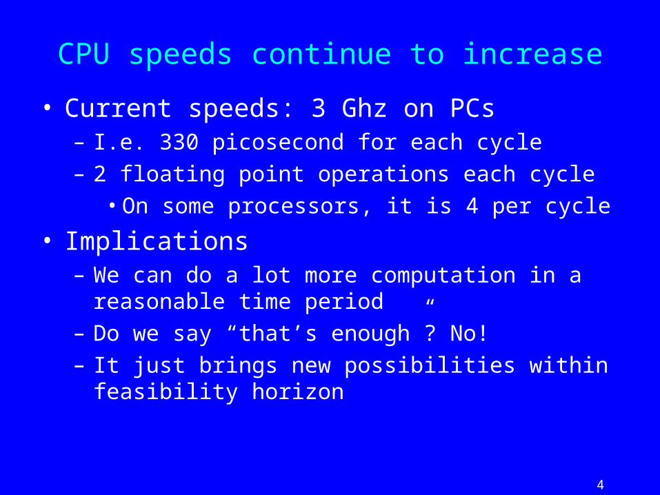
CPU speeds continue to increase

• Current speeds: 3 Ghz on PCs– I.e. 330 picosecond for each cycle

– 2 floating point operations each cycle

• On some processors, it is 4 per cycle

• Implications– We can do a lot more computation in a reasonable time

period

– Do we say “that’s enough”? No!

– It just brings new possibilities within feasibility horizon

5

Parallel Computing Opportunities

• Parallel Machines now– With thousands of powerful processors, at national centers

• ASCI White, PSC Lemieux– Power: 100GF – 5 TF (5 x 1012) Floating Points Ops/Sec

• Japanese Earth Simulator– 30-40 TF!

• Future machines on the anvil– IBM Blue Gene / L – 128,000 processors!– Will be ready in 2004

• Petaflops around the corner

6

Clusters Everywhere

• Clusters with 32-256 processors commonplace in research labs

• Attraction of clusters– Inexpensive

– Latest processors

– Easy to put them together: session this afternoon

• Desktops in a cluster– “Use wasted CPU power”

7

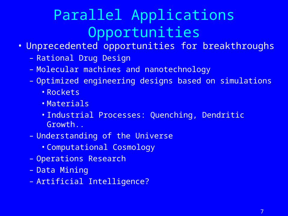
Parallel Applications Opportunities

• Unprecedented opportunities for breakthroughs– Rational Drug Design– Molecular machines and nanotechnology– Optimized engineering designs based on simulations

• Rockets• Materials• Industrial Processes: Quenching, Dendritic Growth..

– Understanding of the Universe• Computational Cosmology

– Operations Research– Data Mining– Artificial Intelligence?

8

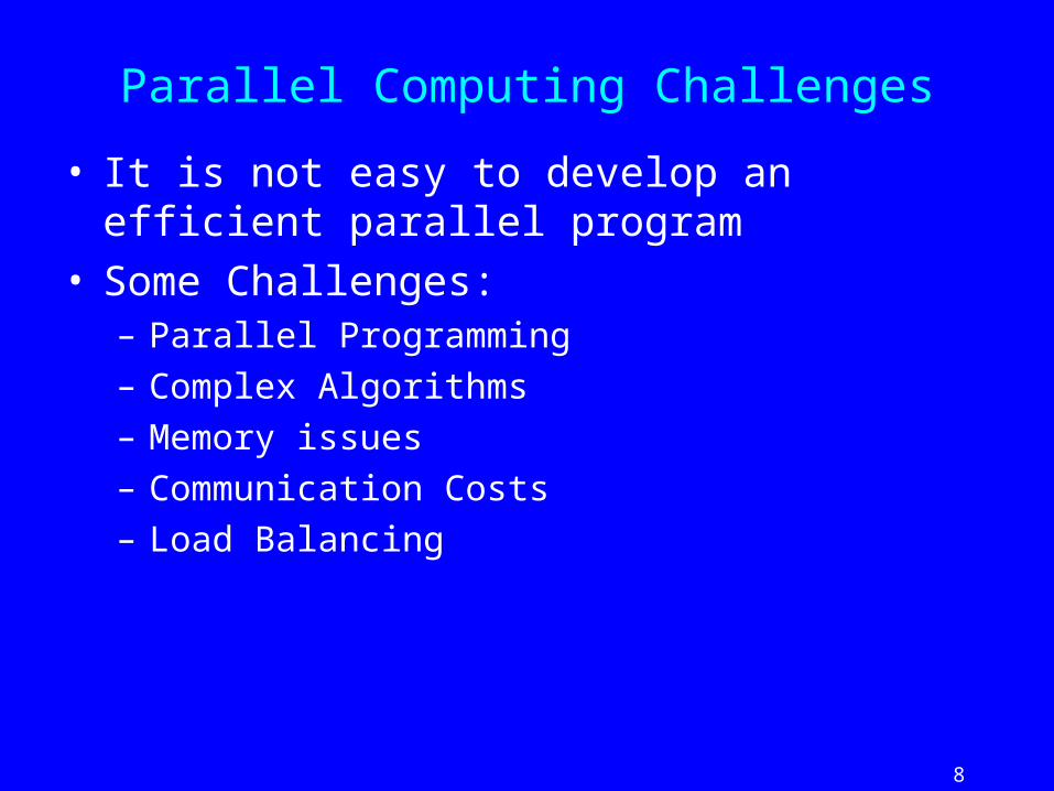
Parallel Computing Challenges

• It is not easy to develop an efficient parallel program• Some Challenges:

– Parallel Programming

– Complex Algorithms

– Memory issues

– Communication Costs

– Load Balancing

9

Why Don’t Applications Scale?• Algorithmic overhead

– Some things just take more effort to do in parallel• Example: Parallel Prefix (Scan)

• Speculative Loss– Do A and B in parallel, but B is ultimately not needed

• Load Imbalance– Makes all processor wait for the “slowest” one– Dynamic behavior

• Communication overhead– Spending increasing proportion of time on communication

• Critical Paths: – Dependencies between computations spread across processors

• Bottlenecks:– One processor holds things up

10

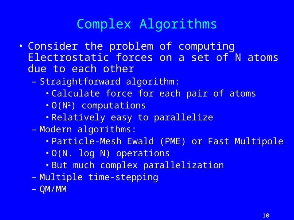
Complex Algorithms

• Consider the problem of computing Electrostatic forces on a set of N atoms due to each other– Straightforward algorithm:

• Calculate force for each pair of atoms• O(N2) computations• Relatively easy to parallelize

– Modern algorithms: • Particle-Mesh Ewald (PME) or Fast Multipole• O(N. log N) operations• But much complex parallelization

– Multiple time-stepping– QM/MM

11

Memory Performance

• DRAM Memory– (the kind you buy from Best Buy) is dense, cheap

– 30-50 nanoseconds to get data from memory into CPU

• CPU can do 2-4 operations every 300 picoseconds– 100+ times slower than CPU!

• Solution:– Memory Hierarchy:

– Use small amount fast but expensive memory (Cache)

– If data fits in Cache, you get Gigaflops performance per proc.

– Otherwise, can be 10-50 times slower!

12

Communication Costs

• Normal Ethernet is slow compared with CPU– Even 100 Mbit ethernet..

• Some basic concepts:– How much data can you get across per unit time: bandwidth

– How much time it needs to send just 1 byte : Latency

– What fraction of this time is spent by the processor?

• CPU overhead

• Problem:– CPU overhead is too high for ethernet

– Because of layers of software and Operating System (OS) involvement

13

Communication Basics: Point-to-point

Sending processor

Sending Co-processor

Network

Receiving co-processor

Receiving processor

Each component has a per-message cost, and per byte cost

Elan-3 cards on alphaservers (TCS):

Of 2.3 μs “put” time1.0 : proc/PCI1.0 : elan card0.2: switch0.1 Cable

14

Communication Basics

• Each cost, for an n-byte message – = ά + n β

• Important metrics: – Overhead at Processor, co-processor

– Network latency

– Network bandwidth consumed

• Number of hops traversed

• Elan-3 TCS Quadrics data:– MPI send/recv: 4-5 μs– Shmem put: 2.5 μs

– Bandwidth : 325 MB/S (about 3 ns per byte)

15

Communication network options

100Mb ethernet Myrinet Quadrics

Latency 100 μs 15 μs 3-5 μs

CPU overhead High Low Low

Bandwidth 5-10 MB 100+ MB 325 MB (about 3 ns/byte)

Cost $ $$$ $$$$

16

1

10

100

1000

0 10000 20000 30000 40000 50000 60000 70000

Message Size (Bytes)

Tim

e (u

s)

Pingpong Compute Time Pingpong Time

Ping Pong Time on Lemieux

Ping Time

Ping CPU Time

10 μs

17

Parallel Programming

• Writing Parallel programs is more difficult than writing sequential programs– Coordination

– Race conditions

– Performance issues

• Solutions:– Automatic parallelization: hasn’t worked well

– MPI: message passing standard in common use

– Processor virtualization:

• Programmer decompose the program into parallel parts, but the system assigns them to processors

– Frameworks: Commonly used parallel patterns are reused

18

Virtualization: Object-based Parallelization

User View

System implementation

User is only concerned with interaction between objects

19

Data driven execution

Scheduler Scheduler

Message Q Message Q

20

Charm++ and Adaptive MPIRealizations of Virtualization Approach

Charm++

• Parallel C++– Asynchronous methods

• In development for over a decade

• Basis of several parallel applications

• Runs on all popular parallel machines and clusters

AMPI

• A migration path for MPI codes – Allows them dynamic load

balancing capabilities of Charm++

• Minimal modifications to convert existing MPI programs

• Bindings for – C, C++, and Fortran90

Both available from http://charm.cs.uiuc.edu

21

Benefits of Virtualization• Software Engineering

– Number of virtual processors can be independently controlled

– Separate VPs for modules

• Message Driven Execution– Adaptive overlap

– Modularity

– Predictability:

• Automatic Out-of-core

• Dynamic mapping– Heterogeneous clusters:

• Vacate, adjust to speed, share

– Automatic checkpointing

– Change the set of processors

• Principle of Persistence:– Enables Runtime

Optimizations

– Automatic Dynamic Load Balancing

– Communication Optimizations

– Other Runtime Optimizations

More info:

http://charm.cs.uiuc.edu

22

NAMD: A Production MD program

NAMD

• Fully featured program

• NIH-funded development

• Distributed free of charge (~5000 downloads so far)

• Binaries and source code

• Installed at NSF centers

• User training and support

• Large published simulations (e.g., aquaporin simulation featured in keynote)

23

NAMD, CHARMM27, PMENpT ensemble at 310 or 298 K 1ns equilibration, 4ns production

Protein:~ 15,000 atomsLipids (POPE): ~ 40,000 atomsWater: ~ 51,000 atomsTotal: ~ 106,000 atoms

3.5 days / ns - 128 O2000 CPUs11 days / ns - 32 Linux CPUs.35 days/ns–512 LeMieux CPUs

Acquaporin Simulation

F. Zhu, E.T., K. Schulten, FEBS Lett. 504, 212 (2001)M. Jensen, E.T., K. Schulten, Structure 9, 1083 (2001)

24

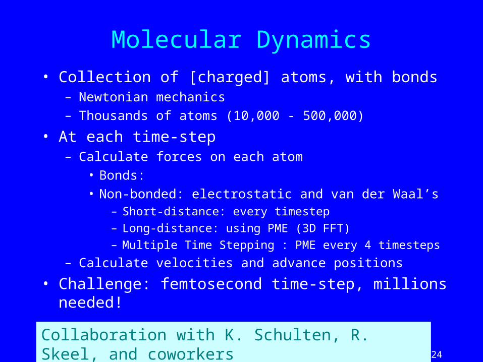
Molecular Dynamics

• Collection of [charged] atoms, with bonds– Newtonian mechanics

– Thousands of atoms (10,000 - 500,000)

• At each time-step– Calculate forces on each atom

• Bonds:

• Non-bonded: electrostatic and van der Waal’s– Short-distance: every timestep

– Long-distance: using PME (3D FFT)

– Multiple Time Stepping : PME every 4 timesteps

– Calculate velocities and advance positions

• Challenge: femtosecond time-step, millions needed!

Collaboration with K. Schulten, R. Skeel, and coworkers

25

Sizes of Simulations Over Time

BPTI3K atoms

Estrogen Receptor36K atoms (1996)

ATP Synthase327K atoms

(2001)

26

Parallel MD: Easy or Hard?

• Easy– Tiny working data

– Spatial locality

– Uniform atom density

– Persistent repetition

– Multiple timestepping

• Hard– Sequential timesteps

– Short iteration time

– Full electrostatics

– Fixed problem size

– Dynamic variations

– Multiple timestepping!

27

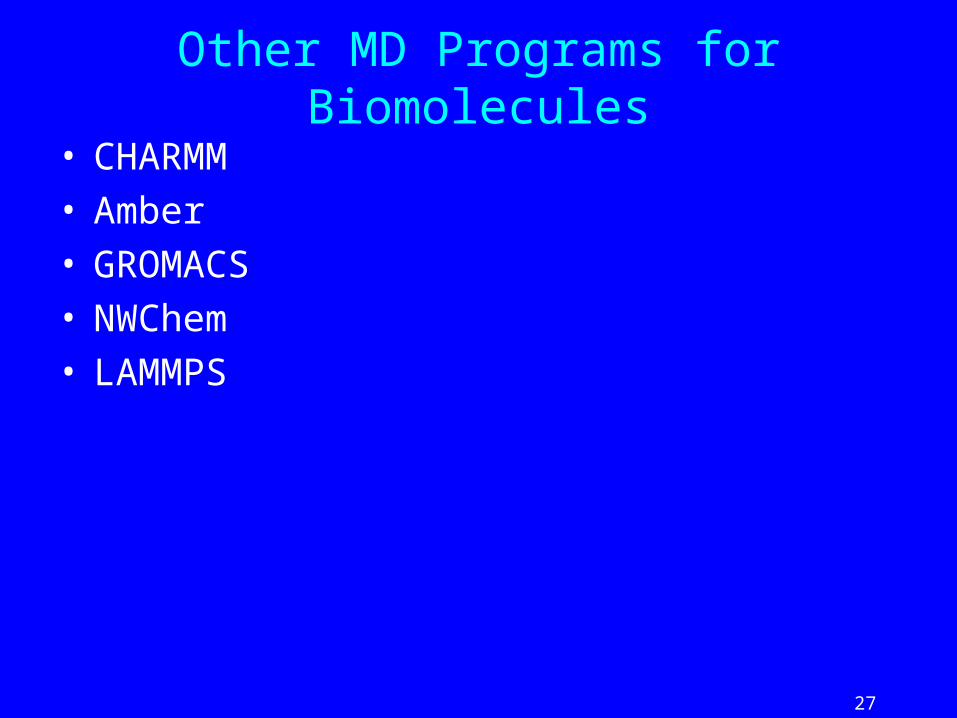
Other MD Programs for Biomolecules

• CHARMM• Amber• GROMACS• NWChem• LAMMPS

28

Scalability

• The Program should scale up to use a large number of processors. – But what does that mean?

• An individual simulation isn’t truly scalable• Better definition of scalability:

– If I double the number of processors, I should be able to retain parallel efficiency by increasing the problem size

29

Scalability

• The Program should scale up to use a large number of processors. – But what does that mean?

• An individual simulation isn’t truly scalable• Better definition of scalability:

– If I double the number of processors, I should be able to retain parallel efficiency by increasing the problem size

30

Isoefficiency

• Quantify scalability• How much increase in problem size is needed to retain

the same efficiency on a larger machine?• Efficiency : Seq. Time/ (P · Parallel Time)

– parallel time = • computation + communication + idle

• Scalability:– If P increases, can I increase N, the problem-size so that the

communication/computation ratio remains the same?

• Corollary:– If communication /computation ratio of a problem of size N

running on P processors increases with P, it can’t scale

31

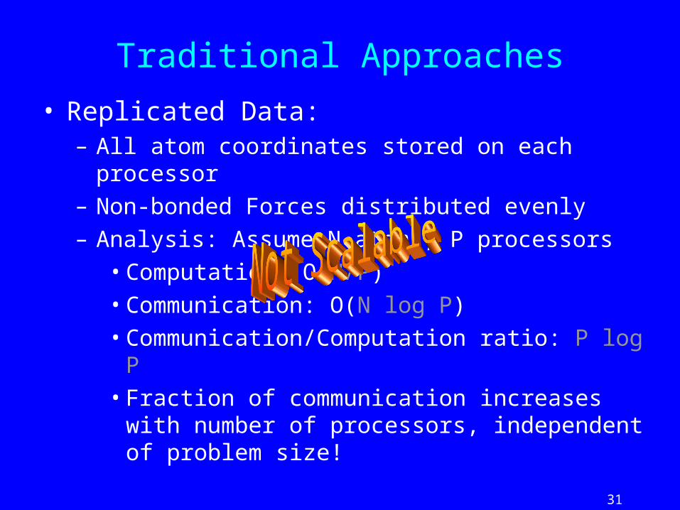
Traditional Approaches

• Replicated Data:– All atom coordinates stored on each processor

– Non-bonded Forces distributed evenly

– Analysis: Assume N atoms, P processors

• Computation: O(N/P)

• Communication: O(N log P)

• Communication/Computation ratio: P log P

• Fraction of communication increases with number of processors, independent of problem size!

32

Atom decomposition

• Partition the Atoms array across processors– Nearby atoms may not be on the same processor

– Communication: O(N) per processor

– Communication/Computation: O(P)

33

Force Decomposition

• Distribute force matrix to processors– Matrix is sparse, non uniform

– Each processor has one block

– Communication: N/sqrt(P)

– Ratio: sqrt(P)

• Better scalability (can use 100+ processors)– Hwang, Saltz, et al:

– 6% on 32 Pes 36% on 128 processor

34

Traditional Approaches: non isoefficient

• Replicated Data:– All atom coordinates stored on each processor

• Communication/Computation ratio: P log P

• Partition the Atoms array across processors– Nearby atoms may not be on the same processor

– C/C ratio: O(P)

• Distribute force matrix to processors– Matrix is sparse, non uniform,

– C/C Ratio: sqrt(P)

35

Spatial Decomposition

• Allocate close-by atoms to the same processor• Three variations possible:

– Partitioning into P boxes, 1 per processor

• Good scalability, but hard to implement

– Partitioning into fixed size boxes, each a little larger than the cutoff disctance

– Partitioning into smaller boxes

• Communication: O(N/P)

36

Spatial Decomposition in NAMD

• NAMD 1 used spatial decomposition• Good theoretical isoefficiency, but for a fixed size

system, load balancing problems• For midsize systems, got good speedups up to 16

processors….• Use the symmetry of Newton’s 3rd law to

facilitate load balancing

37

Spatial Decomposition Via Charm

•Atoms distributed to cubes based on their location

• Size of each cube :

•Just a bit larger than cut-off radius

•Communicate only with neighbors

•Work: for each pair of nbr objects

•C/C ratio: O(1)

•However:

•Load Imbalance

•Limited Parallelism

Cells, Cubes or“Patches”

Charm++ is useful to handle this

38

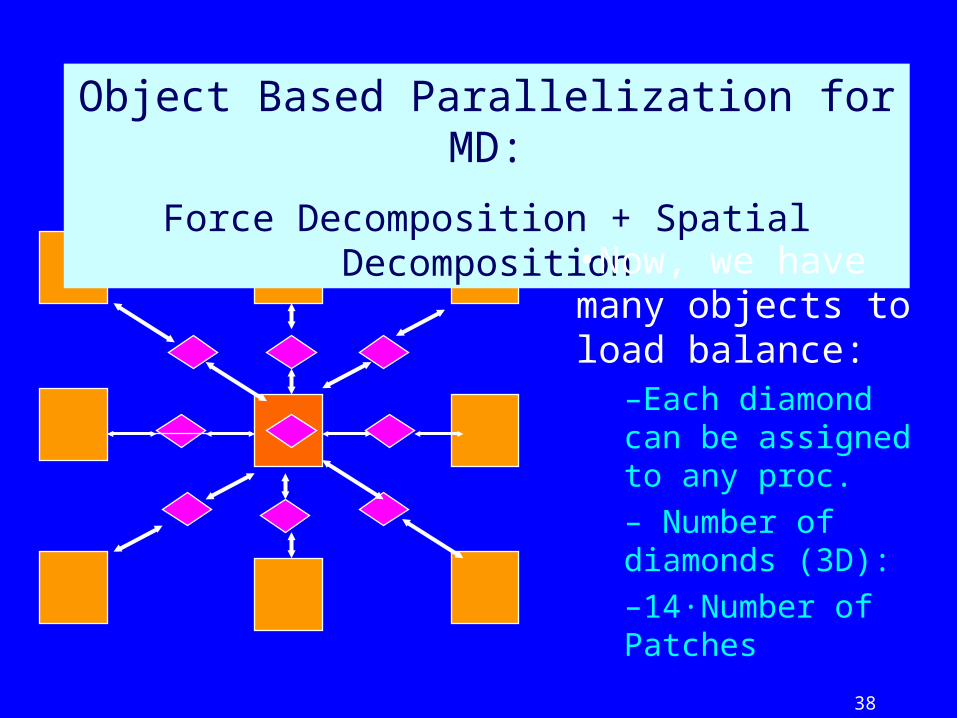
Object Based Parallelization for MD:

Force Decomposition + Spatial Decomposition

•Now, we have many objects to load balance:

–Each diamond can be assigned to any proc.

– Number of diamonds (3D):

–14·Number of Patches

39

Bond Forces

• Multiple types of forces:– Bonds(2), Angles(3), Dihedrals (4), ..

– Luckily, each involves atoms in neighboring patches only

• Straightforward implementation:– Send message to all neighbors,

– receive forces from them

– 26*2 messages per patch!

41

Performance Data: SC2000

Speedup on Asci Red

0

200

400

600

800

1000

1200

1400

0 500 1000 1500 2000 2500

Processors

Sp

eed

up

42

New Challenges

• New parallel machine with faster processors– PSC Lemieux

– 1 processor performance:

• 57 seconds on ASCI red to 7.08 seconds on Lemieux

– Makes is harder to parallelize:

• E.g. larger communication-to-computation ratio

• Each timestep is few milliseconds on 1000’s of processors

• Incorporation of Particle Mesh Ewald (PME)

43

F1F0 ATP-Synthase (ATP-ase)

•CConverts the electrochemical energy of the proton gradient into the mechanical energy of the central stalk rotation, driving ATP synthesis (G = 7.7 kcal/mol).

327,000 atoms total,51,000 atoms -- protein and nucletoide276,000 atoms -- water and ions

The Benchmark

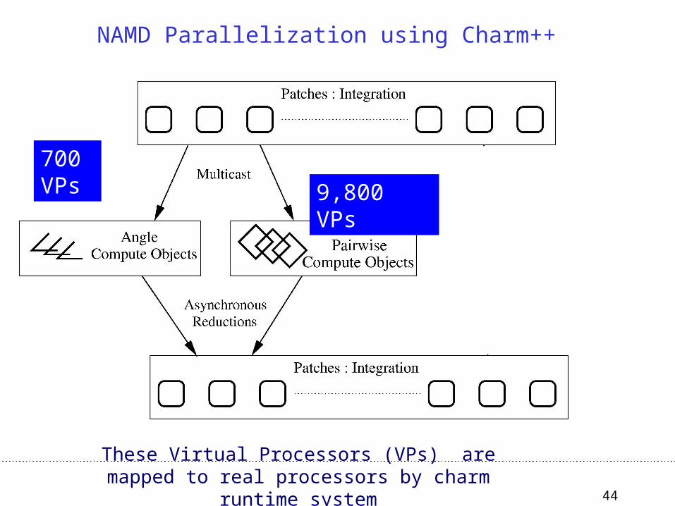
44

700 VPs

NAMD Parallelization using Charm++

These Virtual Processors (VPs) are mapped to real processors by charm runtime system

9,800 VPs

46

Grainsize and Amdahls’s law

• A variant of Amdahl’s law, for objects:– The fastest time can be no shorter than the time for the

biggest single object!

– Lesson from previous efforts

• Splitting computation objects:– 30,000 nonbonded compute objects

– Instead of approx 10,000

47

700 VPs

NAMD Parallelization using Charm++

These 30,000+ Virtual Processors (VPs) are mapped to real processors by charm runtime system

30,000 VPs

48

Mode: 700 us

Distribution of execution times of

non-bonded force computation objects (over 24 steps)

50

Measurement Based Load Balancing

• Principle of persistence– Object communication patterns and computational loads

tend to persist over time

– In spite of dynamic behavior

• Abrupt but infrequent changes

• Slow and small changes

• Runtime instrumentation– Measures communication volume and computation time

• Measurement based load balancers– Use the instrumented data-base periodically to make new

decisions

51

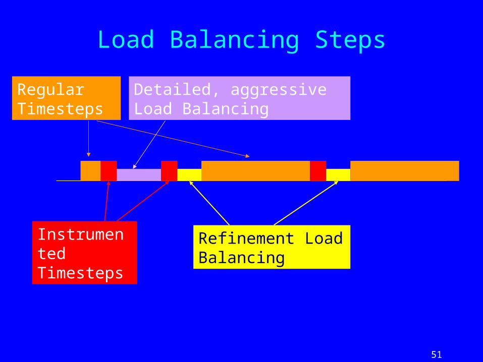
Load Balancing Steps

Regular Timesteps

Instrumented Timesteps

Detailed, aggressive Load Balancing

Refinement Load Balancing

52

Another New Challenge

• Jitter due small variations– On 2k processors or more

– Each timestep, ideally, will be about 12-14 msec for ATPase

– Within that time: each processor sends and receives :

• Approximately 60-70 messages of 4-6 KB each

– Communication layer and/or OS has small “hiccups”

• No problem until 512 processors

• Small rare hiccups can lead to large performance impact– When timestep is small (10-20 msec), AND

– Large number of processors are used

53

Benefits of Avoiding Barrier• Problem with barriers:

– Not the direct cost of the operation itself as much

– But it prevents the program from adjusting to small variations

• E.g. K phases, separated by barriers (or scalar reductions)

• Load is effectively balanced. But,– In each phase, there may be slight non-determistic load imbalance

– Let Li,j be the load on I’th processor in j’th phase.

• In NAMD, using Charm++’s message-driven execution:– The energy reductions were made asynchronous

– No other global barriers are used in cut-off simulations

k

jjii L

1, }{max }{max

1,

k

jjii LWith barrier: Without:

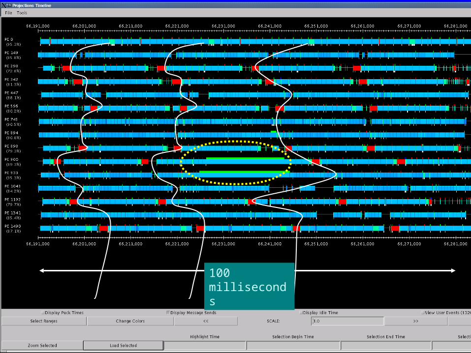
54

100 milliseconds

55

Substep Dynamic Load Adjustments

• Load balancer tells each processor its expected (predicted) load for each timestep

• Each processor monitors its execution time for each timestep – after executing each force-computation object

• If it has taken well beyond its allocated time:– Infers that it has encountered a “stretch”

– Sends a fraction of its work in the next 2-3 steps to other processors

• Randomly selected from among the least loaded processors

migrate Compute(s) away in this step

56

NAMD on Lemieux without PMEProcs Per Node Time (ms) Speedup GFLOPS

1 1 24890 1 0.494

128 4 207.4 119 59

256 4 105.5 236 116

512 4 55.4 448 221

510 3 54.8 454 224

1024 4 33.4 745 368

1023 3 29.8 835 412

1536 3 21.2 1175 580

1800 3 18.6 1340 661

2250 3 14.4 1728 850

ATPase: 327,000+ atoms including water

57

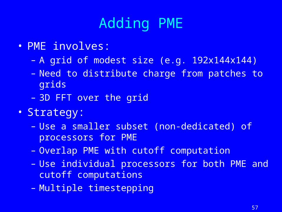
Adding PME

• PME involves:– A grid of modest size (e.g. 192x144x144)

– Need to distribute charge from patches to grids

– 3D FFT over the grid

• Strategy:– Use a smaller subset (non-dedicated) of processors for PME

– Overlap PME with cutoff computation

– Use individual processors for both PME and cutoff computations

– Multiple timestepping

58

700 VPs

192 + 144 VPs

30,000 VPs

NAMD Parallelization using Charm++ : PME

These 30,000+ Virtual Processors (VPs) are mapped to real processors by charm runtime system

59

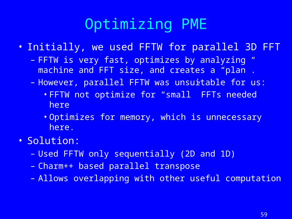
Optimizing PME

• Initially, we used FFTW for parallel 3D FFT– FFTW is very fast, optimizes by analyzing machine and FFT

size, and creates a “plan”.

– However, parallel FFTW was unsuitable for us:

• FFTW not optimize for “small” FFTs needed here

• Optimizes for memory, which is unnecessary here.

• Solution:– Used FFTW only sequentially (2D and 1D)

– Charm++ based parallel transpose

– Allows overlapping with other useful computation

60

Communication Pattern in PME

192

procs

144 procs

61

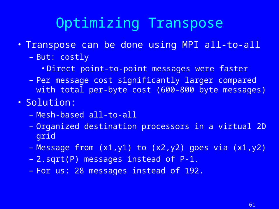
Optimizing Transpose

• Transpose can be done using MPI all-to-all– But: costly

• Direct point-to-point messages were faster

– Per message cost significantly larger compared with total per-byte cost (600-800 byte messages)

• Solution:– Mesh-based all-to-all

– Organized destination processors in a virtual 2D grid

– Message from (x1,y1) to (x2,y2) goes via (x1,y2)

– 2.sqrt(P) messages instead of P-1.

– For us: 28 messages instead of 192.

62

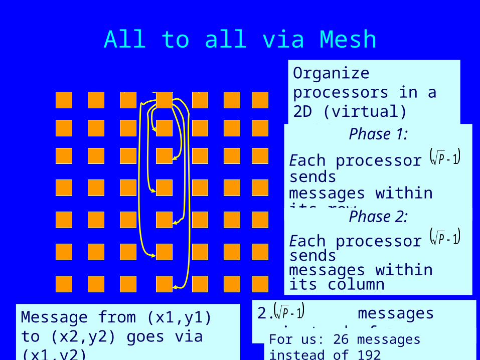
All to all via MeshOrganize processors in a 2D (virtual) grid

Phase 1:

Each processor sends messages within its row

Phase 2:

Each processor sends messages within its column

Message from (x1,y1) to (x2,y2) goes via (x1,y2)

2. messages instead of P-1 1P

For us: 26 messages instead of 192

1P

1P

64

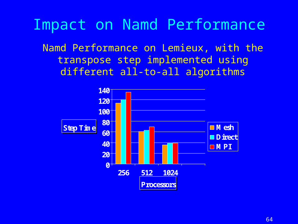
Impact on Namd Performance

0

20

40

60

80

100

120

140

Step Time

256 512 1024

Processors

MeshDirectMPI

Namd Performance on Lemieux, with the transpose step implemented using different all-to-all algorithms

66

Performance: NAMD on Lemieux

Time (ms) Speedup GFLOPSProcs Per Node Cut PME MTS Cut PME MTS Cut PME MTS

1 1 24890 29490 28080 1 1 1 0.494 0.434 0.48128 4 207.4 249.3 234.6 119 118 119 59 51 57256 4 105.5 135.5 121.9 236 217 230 116 94 110512 4 55.4 72.9 63.8 448 404 440 221 175 211510 3 54.8 69.5 63 454 424 445 224 184 213

1024 4 33.4 45.1 36.1 745 653 778 368 283 3731023 3 29.8 38.7 33.9 835 762 829 412 331 3971536 3 21.2 28.2 24.7 1175 1047 1137 580 454 5451800 3 18.6 25.8 22.3 1340 1141 1261 661 495 6052250 3 14.4 23.5 17.54 1728 1256 1601 850 545 770

ATPase: 320,000+ atoms including water

67

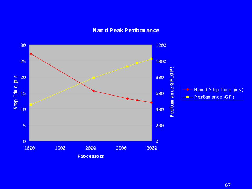
Namd Peak Performance

0

5

10

15

20

25

30

1000 1500 2000 2500 3000

Processors

Ste

p T

ime (

ms)

0

200

400

600

800

1000

1200

Perf

orm

an

ce G

FL

OP

S

Namd Step Time (ms)

Performance (GF)

68

Conclusion: NAMD case study

• We have been able to effectively parallelize MD, – A challenging application

– On realistic Benchmarks

– To 2250 processors, 850 GF, and 14.4 msec timestep

– To 2250 processors, 770 GF, 17.5 msec timestep with PME and multiple timestepping

• These constitute unprecedented performance for MD– 20-fold improvement over our results 2 years ago

– Substantially above other production-quality MD codes for biomolecules

• Using Charm++’s runtime optimizations• Automatic load balancing

• Automatic overlap of communication/computation– Even across modules: PME and non-bonded

• Communication libraries: automatic optimization