1 inverse problems and parameter identiﬁcation in image...

1

Inverse Problems and Parameter Identification

in Image Processing

Michail Kulesh1, Benjamin Berkels2, Kristian Bredies3, Christoph Garbe4,Jens F. Acker5, Mamadou S. Diallo6, Marc Droske2, MatthiasHolschneider1, Jaroslav Hron5, Claudia Kondermann4, Peter Maass3,Nadine Olischlager2, Heinz-Otto Peitgen7, Tobias Preusser7, MartinRumpf2, Frank Scherbaum8, and Stefan Turek5

1 Institute for Mathematics, University of Potsdam,Am Neuen Palais 10, 14469 Potsdam, Germanymkulesh,[email protected]

2 Institute for Numerical Simulation, University of Bonn,Wegelerstr. 6, 53115 Bonn, Germanybenjamin.berkels,nadine.olischlaeger,[email protected]

3 Center of Industrial Mathematics (ZeTeM), University of Bremen,Postfach 33 04 40, 28334 Bremen, Germanykbredies,[email protected]

4 Interdisciplinary Center for Scientific Computing, University of Heidelberg,Im Neuenheimer Feld 368, 69120 Heidelberg, GermanyChristoph.Garbe,[email protected]

5 Institute for Applied Mathematics, University of Dortmund, Vogelpothsweg 87,44227 Dortmund, Germanyjens.acker,jaroslav.hron,[email protected]

6 Now at ExxonMobil Upstream Research company, Houston, Texas, [email protected]

7 Center for Complex Systems and Visualization, University of Bremen,Universitatsallee 29, 28359 Bremen, Germanyheinz-otto.peitgen,[email protected]

8 Institute for Geosciences, University of Potsdam, Karl-Liebnecht-Strasse 24,14476 Potsdam, Germany [email protected]

1.1 Introduction

Many problems in imaging are actually inverse problems. One reason for thisis that conditions and parameters of the physical processes underlying theactual image acquisition are usually not known. Examples for this are theinhomogeneities of the magnet field in magnetic resonance images leading tononlinear deformations of the anatomic structures in the recorded images,material parameters in geological structures as unknown parameters for thesimulation of seismic wave propagation with sparse measurement on the sur-

2 Kulesh, Berkels, Bredies, Garbe, Acker et al.

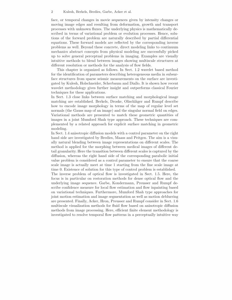
face, or temporal changes in movie sequences given by intensity changes ormoving image edges and resulting from deformation, growth and transportprocesses with unknown fluxes. The underlying physics is mathematically de-scribed in terms of variational problem or evolution processes. Hence, solu-tions of the forward problem are naturally described by partial differentialequations. These forward models are reflected by the corresponding inverseproblems as well. Beyond these concrete, direct modeling links to continuummechanics abstract concepts from physical modeling are successfully pickedup to solve general perceptual problems in imaging. Examples are visuallyintuitive methods to blend between images showing multiscale structures atdifferent resolution or methods for the analysis of flow fields.

This chapter is organized as follows. In Sect. 1.2 wavelet based methodfor the identification of parameters describing heterogeneous media in subsur-face structures from sparse seismic measurements on the surface are investi-gated by Kulesh, Holschneider, Scherbaum and Diallo. It is shown how recentwavelet methodology gives further insight and outperforms classical Fouriertechniques for these applications.In Sect. 1.3 close links between surface matching and morphological imagematching are established. Berkels, Droske, Olischlager and Rumpf describehow to encode image morphology in terms of the map of regular level setnormals (the Gauss map of an image) and the singular normal field on edges.Variational methods are presented to match these geometric quantities ofimages in a joint Mumford Shah type approach. These techniques are com-plemented by a related approach for explicit surface matching in geometricmodeling.In Sect. 1.4 anisotropic diffusion models with a control parameter on the righthand side are investigated by Bredies, Maass and Peitgen. The aim is a visu-ally natural blending between image representations on different scales. Themethod is applied for the morphing between medical images of different de-tail granularity. Here the transition between different scales is captured by thediffusion, whereas the right hand side of the corresponding parabolic initialvalue problem is considered as a control parameter to ensure that the coarsescale image is actually meet at time 1 starting from the fine scale image attime 0. Existence of solution for this type of control problem is established.The inverse problem of optical flow is investigated in Sect. 1.5. Here, thefocus is in particular on restoration methods for dense optical flow and theunderlying image sequence. Garbe, Kondermann, Preusser and Rumpf de-scribe confidence measure for local flow estimation and flow inpainting basedon variational techniques. Furthermore, Mumford Shah type approaches forjoint motion estimation and image segmentation as well as motion deblurringare presented. Finally, Acker, Hron, Preusser and Rumpf consider in Sect. 1.6multiscale visualization methods for fluid flow based on anisotropic diffusionmethods from image processing. Here, efficient finite element methodology isinvestigated to resolve temporal flow patterns in a perceptually intuitive way

1 Inverse Problems and Parameter Identification in Image Processing 3

based on time dependent texture mapping. In addition algebraic multigridmethods are applied for a hierarchical clustering of flow pattern.

1.2 Inverse Problems and Parameter Identification in

Geophysical Signal Processing

Surface wave propagation in heterogeneous media can provide a valuablesource of information about the subsurface structure and its elastic prop-erties. For example, surface waves can be used to obtain subsurface rigiditythrough inversion of the shear wave velocity. The processing of experimentalseismic data sets related to the surface waves is computationally expensiveand requires sophisticated techniques in order to infer the physical propertiesand structure of the subsurface from the bulk of available information.

Most of the previous studies related to these problems are based on Fourieranalysis. However, the frequency-dependent measurements, or time-frequencyanalysis (TFR) offer additional insight and performance in any applicationswhere Fourier techniques have been used. This analysis consists of examiningthe variation of the frequency content of a signal with time and is particularlysuitable in geophysical applications.

The continuous wavelet transform (CWT) of a real or complex signalS(t) ∈ L2(R) with respect to a real or complex mother wavelet is the setof L2–scalar products of all dilated and translated wavelets with this sig-nal Holschneider [1995]:

WgS(t, a) = 〈TtDag, S〉 =

+∞∫

−∞

1

ag∗

(τ − t

a

)

S(τ) dτ ,

S(t) = MhWgS(t, a) =1

Cg,h

+∞∫

−∞

+∞∫

−∞

h

(

t− τ

a

)

WgS(τ, a)dτ da

a2,

(1.1)

where g, h are wavelets used for the direct and inverse wavelet transforms,Da : g(τ) 7→ g(τ/a)/a and Tt : g(τ) 7→ g(τ − t) define the dilation a ∈ R andtranslation t ∈ R operations correspondingly. If we select a wavelet with aunit central frequency, it is possible to obtain the physical frequency directlyby taking the inverse of the scale: f = 1/a.

This approach is powerful and elegant, but is not the only one availablefor practical applications. Other TFR methods such as the Gabor transform,the S-transform Schimmel and Gallart [2005] or bilinear transforms like theWigner-Ville Pedersen et al. [2003] or smoothed Wigner-Ville transform canbe used as well. The relative performance of time-frequency analysis fromdifferent TFR approaches is primarily controlled by the frequency resolutioncapability that motivated the use of CWT in the present work.

With multicomponent data, one is usually confronted with the issue of sep-arating seismic signals of different polarization characteristics. For instance,


one would like to distinguish between the body waves (P- and S- waves) thatare linearly polarized from elliptically polarized Rayleigh waves. Polarizationanalysis is also used to identify shear wave splitting. Unfortunately, there isno mathematically exact a priori definition for the instantaneous polarizationattributes of a multicomponent signal. Therefore any attempts to produce oneare usually arbitrary.

Time-frequency representations can be incorporated in polarization anal-ysis Soma et al. [2002], Schimmel and Gallart [2005], Pinnegar [2006]. Weproposed several different wavelet based methods for the polarization analysisand filtering.

1.2.1 Polarization Properties for Two-Component Data

Given a signal from three-component record, with Sx(t), Sy(t), and Sz(t)representing the seismic traces recorded in three orthogonal directions, anycombination of two orthogonal components can be selected for the polar-ization analysis: Z(t) = Sk(t) + iSm(t). Let us consider the instantaneousangular frequency defined as the derivative of the complex spectrum’s phase:Ω±(t, f) = ±∂ argW±

g Z(t, f)/∂t. Then, near time instant t, each componentcan be represented as follows:

WgZ(t+ τ, f) ≃ W+g Z(t, f)eiΩ+(t,f)τ + W−

g Z(t, f)e−iΩ−(t,f)τ ,

which yields the time-frequency spectrum for each of the parameters (see Kuleshet al. [2005b], Diallo et al. [2006b]):

R(t, f) = |W+g Z(t, f)| + |W−

g Z(t, f)|/2 ,

r(t, f) = ||W+g Z(t, f)| − |W−

g Z(t, f)||/2 ,

θ(t, f) = arg[W+g Z(t, f)W−

g Z(t, f)]/2 ,

∆φ(t, f) = arg(

W+g Z(t,f)+W−

g Z(t,f)∗

W+g Z(t,f)−W−

g Z(t,f)∗

)

modπ ,

(1.2)

where R is the semi-major axis R ≥ 0, r is the semi-minor axis R ≥ r ≥ 0, θis the tilt angle, which is the angle of the semi-major axis with the horizontalaxis, θ ∈ (−π/2, π/2] and ∆φ is the phase difference between Sk(t) and Sm(t)components.

If we analyze seismic data, an advantage of the method (1.2) is the possi-bility to perform the complete wave-mode separation/filtering process in thewavelet domain and the ability to provide the frequency dependence of el-lipticity, which contains important information on the subsurface structure.With the extension of the polarization analysis to the wavelet domain, wecan construct filtering algorithms to separate different wave types based onthe instantaneous attributes by a combination of constraints posed on therange of the reciprocal ellipticity ρ(t, f) = r(t, f)/R(t, f) and the tilt angleθ(t, f) Diallo et al. [2006b].


1.2.2 Polarization Properties for Three-Component Data

Reference Morozov and Smithson [1996] proposed a method based on a vari-ational principle that allows generalization to any number of components,and they briefly addressed the possibility of using the instantaneous polariza-tion attributes for wavefield separation and shear-wave splitting identification.In Diallo et al. [2005], we extended the method of Morozov and Smithson[1996] to the wavelet domain in order to use the instantaneous attributes forfiltering and wavefield separation for any number of components. As an exam-ple, Pacor et al. [2007] used this method for spectral analysis and multicompo-nent polarization analyses on the Gubbio Piana (central Italy) recordings toidentify the frequency content of the different phases composing the recordedwavefield and to highlight the importance of basin-induced surface waves inmodifying the main strong ground-motion parameters.

In more general terms, particle motions captured with three-componentrecordings can be characterized by a polarization ellipsoid. Several meth-ods are proposed in the literature to introduce such an approximation.They are based on the analysis of the covariance matrix of multicomponentrecordings and principal components analysis using singular value decompo-sition Kanasewich [1981]. In Kulesh et al. [2007a], we extended the covariancemethod to the time-frequency domain. Following the method, proposed by Di-allo et al. [2006a], we use an approximate analytical formula to compute theelements of the covariance matrix M(t, f) for a time window which is derivedfrom an averaged instantaneous frequency of the multicomponent record:

Mkm(t, f) = |WgSk(t, f)| |WgSm(t, f)| sinc (Γ−km(t, f)) cos (A−

km(t, f))

+ sinc (Γ+km(t, f)) cos (A+

km(t, f)) − µkmµmk ,

Γ±km(t, f) = ∆tkm(t,f)

2 (Ωk(t, f) ±Ωm(t, f)) ,

A±km(t, f) = argWgSk(t, f) ± argWgSm(t, f) ,

∆tkm(t, f) = 4πnΩk(t,f)+Ωm(t,f) , n ∈ N ,

µkb = ℜ [WgSk(t, f)] sinc (∆tkb(t,f)Ωk(t,f)2 ) , k,m = x, y, z,

(1.3)

where sinc(x) indicates the sine cardinal function.The eigenanalysis performed on M(t, f) yields the principal component

decomposition of the energy. Such a decomposition produces three eigenval-ues λ1(t, f) ≥ λ2(t, f) ≥ λ3(t, f) and three corresponding eigenvectors vk(t, f)that fully characterize the magnitudes and directions of the principal compo-nents of the ellipsoid that approximates the particle motion in the consideredtime window ∆tkm(t, f):

• the major half-axis R(t, f) =√

λ1(t, f)v1(t, f)/‖v1(t, f)‖ ;

• the minor half-axis r(t, f) =√

λ3(t, f)v3(t, f)/‖v3(t, f)‖ ;


• the second minor half-axis rs(t, f) =√

λ2(t, f)v2(t, f)/‖v2(t, f)‖ ;

• the reciprocal ellipticity ρ(t, f) = ‖rs(t, f)‖/‖R(t, f)‖ ;

• the minor reciprocal ellipticity ρ1(t, f) = ‖r(t, f)‖/‖rs(t, f)‖ ;

• the dip angle δ(t, f) = arctan(√

v1,x(t, f)2 + v1,y(t, f)2/v1,z(t, f)) ;

• the azimuth α(t, f) = arctan(v1,y(t, f)/v1,x(t, f)) .

Note, when the instantaneous frequencies are the same for all components,this method produces the same results as those by Morozov and Smithson[1996] in terms of polarization parameters.

1.2.3 Modeling a Wave Dispersion Using a Wavelet DeformationOperator

The second problem in the context of surface wave analysis (especially withhigh frequency signals) is the robust determination of dispersion curves frommultivariate signals. Wave dispersion expresses the phenomenon by which thephase and group velocities are functions of the frequency. The cause of dis-persion may be either geometric or intrinsic. For seismic surface waves, thecause of dispersion is of a geometrical nature. Geometric dispersion resultsfrom the constructive interferences of waves in bounded or heterogeneous me-dia. Intrinsic dispersion arises from the causality constraint imposed by theKramers-Kronig relation or from the microstructure properties of material. Ifthe dispersive and dissipative characteristics of the medium are represented bythe frequency-dependent wavenumber k(f) and attenuation coefficient α(f),the relation between the Fourier transforms of two propagated signals reads

O[DF ] : S(f) 7→ e−iK(f)D−2πinS(f) ,

where D is the propagation distance, n ∈ N is any integer number and K(f)is the complex wavenumber, which can be defined by real functions k(f) andα(f) as K(f) = 2πk(f) − iα(f) .

In order to analyze the dynamical behavior of multivariate signals using thecontinuous wavelet transforms it is interesting to investigate a diffeomorphicdeformation of the wavelet space. These deformations establish algebra ofwavelet pseudodifferential operators acting on signals Xie et al. [2003]. In themost general case, a wavelet deformation operator can be defined as

O[D] : S(t) 7→ MhDWgS(t, f) , D : H → H ,H := (t, f) : t ∈ R, f > 0 .

We investigated some practical models that give concreted expression ofthis deformation operator related to the used dispersion parameters of themedium. Reference Kulesh et al. [2005a] has shown how the wavelet trans-form of the source and the propagated signals are related through a transfor-mation operator that explicitly incorporates the wavenumber as well as theattenuation factor of the medium:


O[DW ] : WgS(t, f) 7→ e−α(f)De−iψ1(f)WgS (t− k′(f)D, f) , (1.4)

where ψ1(f) = 2π[k(f) − fk′(f)]D + 2πn.In the special case, with the assumption that the analyzing wavelet has a

linear phase (with time-derivative approximately equal to 2π, as it is the casefor the Morlet wavelet, the approximation (1.4) can be written in terms of thephase Cp(f) = f/k(f) and group Cg(f) = 1/k′(f) velocities as Kulesh et al.[2005b]:

O[DW ] : WgS(t, f) 7→ e−α(f)D∣

∣

∣WgS

(

t− DCg(f) , f

)∣

∣

∣·

exp[

i argWgS(

t− DCp(f) −

nf , f

)]

.(1.5)

The relationship (1.5) has the following interpretation. The group velocity is afunction that “deforms” the image of the absolute value of the source signal’swavelet spectrum, the phase velocity ”deforms” the image of the wavelet spec-trum phase, and the attenuation function determines the frequency-dependentreal coefficient by which the spectrum is multiplied.

1.2.4 How to Extract the Dispersion Properties from the WaveletCoeffitients?

Equation (1.5) allows us to formulate the ideas how the frequency-dependentdispersion properties can be obtained using the wavelet spectra’ phases ofsource and propagated signals. To obtain the phase velocities of multi-modeand multivariate signals, we can perform ”frequency-velocity” analysis on theanalogy of the frequency-wavenumber method Capon [1969] for a seismogramSk(t) , k = 1, N . The main part of this analysis consists of the calculation ofcorrelation spectrum M(f, c) as follows (see Kulesh et al. [2007b]):

M(f, c) =

∫ tmax

tmin

∣

∣

∣

∣

∣

∑

k,m

Ak(τ, f)A∗m

(

τ −Dmk

c, f

)

∣

∣

∣

∣

∣

dτ

=

∫ tmax

tmin

∣

∣

∣

∣

∣

∑

k,m

eiBk(τ,f) exp

(

−iBm

(

τ −Dmk

c, f

))

∣

∣

∣

∣

∣

dτ ,

Ak(τ, f) = WgSk(τ, f)/|WgSk(τ, f)|, Bk(τ, f) = argWgSk(τ, f) ,

(1.6)

where [tmin, tmax] indicates the total time range for which the wavelet spec-trum was calculated, c ∈ [Cminp , Cmaxp ] is an unbounded variable correspond-ing to the phase velocity, Ak is a complex-valued wavelet phase and Bk is areal-valued wavelet phase.

For a given parametrization of wavenumber and attenuation functions,finding an acceptable set of parameters can be thought of as an optimizationproblem that seeks to minimize a cost function χ2 and can be formulated asfollows:


χ2(α(f,p), k(f,q)) → min , p ∈ RP , q ∈ R

Q ,

where P is the number of parameters used to model the attenuation α(f) andQ is the number of parameters used to model the wavenumber k(f). p andq represent the vectors of parameters describing α(f) and k(f) respectively.This cost function involves a propagator described above.

At this stage we need to distinguish between the case where the analyzedsignal consists only of one coherent arrival from the case where it consists ofseveral coherent arrivals. In the former case, the derived functions are mean-ingful and characterize those analyzed event. However in the latter, thesefunctions cannot be easily interpreted since the signals involved consist ofmany overlapping arrivals.

If only one single phase is observed in all the traces Sk(t), it will be enoughto minimize a cost function that involves some selected seismic traces in orderto estimate the attenuation and phase velocity using the modulus and thephase of the wavelet transforms correspondingly, see Holschneider et al. [2005]:

χ2(p,q) =∑

m,k

∫ ∫

||WgSk(t, f)| − |DW(p,q)WgSm(t, f)||2

dt df ,

χ2(p,q) =∑

m,k

∫ ∫

|argWgSk(t, f) − argDW(p,q)WgSm(t, f)|2

dt df .

(1.7)The first step will consist of seeking a good initial condition by performing animage matching using the modulus of the wavelet transforms of a pair of traces.The optimization is carried out over the whole frequency range of the signal. Inorder to reduce the effect of uncorrelated noise in our estimates, it is preferableto use a propagator based on the cross-correlations, see Holschneider et al.[2005].

In the case where the observed signals consist of a mixture of differentwave types and modes, a cascade of optimizations in the wavelet domainwill be necessary in order to fully determine the dispersion and attenuationcharacteristics specific to each coherent arrival.

Since the dependence of the cost functions (1.7) on the parameters p and qis highly non-linear, each function may have several local minima. To obtainthe global minimum that corresponds to the true parameters, a non-linearleast-squares minimization method that proceeds iteratively from a reasonableset of initial parameters is required. In the present contribution, we use theLevenberg-Marquardt algorithm Press et al. [1992].

Finally, the obtained dispersion curves (especially phase and group veloc-ities) for defined wave types can be used for the determination of physicaland geometrical properties of the subsurface structure. Because of the non-uniqueness of earth models that can be fitted to a given dispersion curve,the inversion for the average shear velocity profile is usually treated as anoptimization problem where one tries to minimize the misfit between exper-


imental and theoretical dispersion curves computed for a given earth modelthat is assumed to best represent the subsurface under investigation.

1.3 The Interplay of Image Registration and Geometry

Matching

Image registration is one of the fundamental tools in image processing. Itdeals with the identification of structural correspondences in different imagesof the same or of similar objects acquired at different times or with differentimage devices. For instance, the revolutionary advances in the development ofimaging modalities has enabled clinical researchers to perform precise studiesof the immense variability of human anatomy. As described in the excellentreview by Miller, Trouve and Younes Miller et al. [2002] and the overview ar-ticle of Grenander and Miller Grenander and Miller [1998], this field aims atautomatic detection of anatomical structures and their evaluation and com-parison. Different images show corresponding structures at usually nonlinearlytransformed positions.

In image processing, registration is often approached as a variational prob-lem. One asks for a deformation φ on an image domain Ω which maps struc-tures in the reference image uR onto corresponding structures in the templateimage uT . This leads ill-posed minimization problem if one considers the in-finite dimensional space of deformations Brown [1992]. A iterative, multilevelregularization of the descent direction has been investigated in Clarenz et al.[2006]. Alternatively, motivated by models from continuum mechanics, the de-formation can additionally be controlled by elastic stresses on images regardedas elastic sheets. For example see the early work of Bajcsy and Broit Bajcsyand Broit [1982] and more recent, significant extensions by Grenander andMiller Grenander and Miller [1998]. In Droske and Rumpf [2004] nonlinearelasticity based on polyconvex energy functionals is investigated to ensure aone-to-one image matching. As the image modality differs there is usually nocorrelation of image intensities at corresponding positions. What still remains,at least partially, is the local geometric image structure or “morphology” ofcorresponding objects. Viola, Wells et al. Viola and Wells [1997] and Col-lignon Collignon and et al. [1995] presented an information theoretic approachfor the registration of multi-modal images. Here, we consider “morphology” asa geometric entity and will review registration approaches presented in Droskeand Ring [2007], Droske and Rumpf [2004, 2005].

Obviously, geometry matching is also a widespread problem in computergraphics and geometric modeling Gu and Vemuri [2004]. E.g. motivated bythe ability to scan geometry with high fidelity, a number of approaches havebeen developed in the graphics literature to bring such scans into correspon-dence Blanz and Vetter [1999], Lee et al. [1999]. Given a reference surface MR

and a template surface MT a particular emphasize is on the proper alignment


of curved features and the algorithmic issues associated with the manage-ment of irregular meshes and their effective overlay. Here, we will describean image processing approach to the nonlinear elastic matching of surfacepatches Litke et al. [2005]. It is based on a proper variational parametrizationmethod Clarenz et al. [2004] and on the matching of surface characteristicsencoded as images uR and uT on flat parameter domains ωR and ωT , respec-tively. Here, it is particularly important to take into account of the metricdistortion, to ensure a physically reasonable matching of the actual surfacesMR and MT .

1.3.1 The Geometry of Images

In mathematical terms, two images u, v : Ω → R with Ω ⊂ Rd for d =

2, 3 are called morphologically equivalent, if they only differ by a changeof contrast, i.e. , if u(x) = (βv)(x) for all x ∈ Ω and for some monotonefunction β : R → R. Obviously, such a contrast modulation does not changethe order and the shape of super level sets l+c [u] = x : u(x) ≥ c . Thus,image morphology can be defined as the upper topographic map, defined asthe set of all these sets morph[u] := l+c [u] : c ∈ R . Unfortunately, this setbased definition is not feasible for a variational approach and it does notdistinguish between edges and level sets in smooth image regions. Hence, inwhat follows, we derive an alternative notion and consider image functionsu : Ω → R in SBV Ambrosio et al. [2000] - by definition L1 functions, whosederivative Du is a vector-valued Radon measure with vanishing Cantor part.We consider the usual splitting Du = Dacu + Dju Ambrosio et al. [2000],where Dacu is the regular part, which is the usual image gradient apart fromedges and absolutely continuous with respect to the Lebesgue measure L,and a singular part Dju, which represents the jump and is defined on thejump set J , which consists of the edges of the image. We denote by nj thevector valued measure representing the normal field on J . Obviously, nj isa morphological invariant. For the regular part of the derivative we adoptthe classical gradient notion ∇acu for the L density of Dacu, i.e., Dacu =∇acuL Ambrosio et al. [2000]. As long as it is defined, the normalized gradient∇acu(x) / ‖∇acu(x)‖ is the outer normal on the upper topographic set l+u(x)[u]

and thus again a morphological quantity. It is undefined on the flat imageregion F [u] := x ∈ Ω : ∇acu(x) = 0 . We introduce nac as the normalizedregular part of the gradient nac = χ

Ω\F [u]∇acu / ‖∇acu‖ . We are now able to

redefine the morphology morph[u] of an image u as a unit length vector valuedRadon measure on Ω with morph[u] = nacL + ns . We call nacL the regularmorphology or Gauss map (GM) and ns the singular morphology. In the nextsection, we aim to measure congruence of two image morphologies with respectto a matching deformation making explicit use of this decomposition.


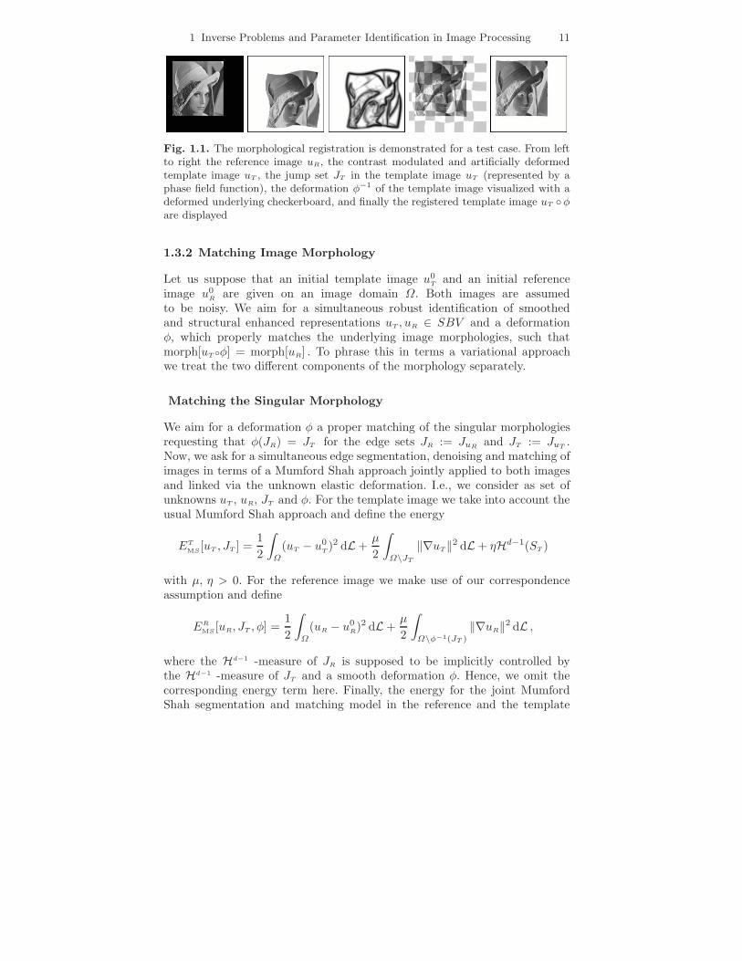
Fig. 1.1. The morphological registration is demonstrated for a test case. From leftto right the reference image uR, the contrast modulated and artificially deformedtemplate image uT , the jump set JT in the template image uT (represented by aphase field function), the deformation φ−1 of the template image visualized with adeformed underlying checkerboard, and finally the registered template image uT φ

are displayed

1.3.2 Matching Image Morphology

Let us suppose that an initial template image u0T

and an initial referenceimage u0

Rare given on an image domain Ω. Both images are assumed

to be noisy. We aim for a simultaneous robust identification of smoothedand structural enhanced representations uT , uR ∈ SBV and a deformationφ, which properly matches the underlying image morphologies, such thatmorph[uT φ] = morph[uR] . To phrase this in terms a variational approachwe treat the two different components of the morphology separately.

Matching the Singular Morphology

We aim for a deformation φ a proper matching of the singular morphologiesrequesting that φ(JR) = JT for the edge sets JR := JuR and JT := JuT .Now, we ask for a simultaneous edge segmentation, denoising and matching ofimages in terms of a Mumford Shah approach jointly applied to both imagesand linked via the unknown elastic deformation. I.e., we consider as set ofunknowns uT , uR, JT and φ. For the template image we take into account theusual Mumford Shah approach and define the energy

ET

MS[uT , JT ] =

1

2

∫

Ω

(uT − u0T)2 dL +

µ

2

∫

Ω\JT

‖∇uT‖2 dL + ηHd−1(ST )

with µ, η > 0. For the reference image we make use of our correspondenceassumption and define

ER

MS [uR, JT , φ] =1

2

∫

Ω

(uR − u0R)2 dL +

µ

2

∫

Ω\φ−1(JT )

‖∇uR‖2 dL ,

where the Hd−1 -measure of JR is supposed to be implicitly controlled bythe Hd−1 -measure of JT and a smooth deformation φ. Hence, we omit thecorresponding energy term here. Finally, the energy for the joint MumfordShah segmentation and matching model in the reference and the template


Fig. 1.2. The registration of FLAIR and T1-weighted magnetic resonance brainimages is considered. From left to right: the reference T1 weighted MR image uR,the template FLAIR image uT , the initial mismatch (with alternating stripes fromuT and uR), and in the same fashion results for a registration only of the regularmorphology and finally for the complete energy are shown

image is given by EMS [uR, uT , ST , φ] = ETMS

[uT , JT ] + ERMS

[uR, JT , φ] . So far,the deformation φ is needed only on the singularity set ST and thus it is highlyunder determined.

Matching the Regular Morphology

The regular image morphology consists of the normal field nac. Given regu-larized representations uT and uR of noisy initial images we observe a perfectmatch of the corresponding regular morphologies, if the deformation of the ref-erence normal field nac

R:= ∇acuR / ‖∇

acuR‖ coincides with the template nor-mals field nacT := ∇acuT / ‖∇

acuT‖ at the deformed position. In fact, all levelsets of the pull back template image uT φ and the reference image uR wouldthen be nicely aligned. In the context of a linear mapping A normals deformedwith the inverse transpose A−T , Thus, we obtain the deformed reference nor-mal nac,φR = CofDφ∇acuR / ‖CofDφ∇acuR‖ , where Cof A := detAA−T and

ask for a deformation φ : Ω → Rd, such that nacT φ = nac,φR . This can be

phrased in terms of an energy integrand g0 : Rd ×Rd × Rd,d → R

+0 , which is

zero-homogeneous in the first two arguments as long as they both do not van-ish and zero elsewhere. It measures the misalignment of directions of vectorson Rd. For instance we might define

g0(w, z,A) := γ

∥

∥

∥

∥

(1−w

‖w‖⊗

w

‖w‖)

Cof Az

‖Cof Az‖

∥

∥

∥

∥

m

for w, z 6= 0, with γ > 0 and m ≥ 2, a⊗ b = abT . Based on this integrand wefinally define a Gauss map registration energy

EGM [uT , uR, φ] =

∫

Ω

g0(DacuT φ,DacuR,CofDφ) dL .

For the analytical treatment of the corresponding variational problem we referto Droske and Rumpf [2004].

In a variational setting neither the matching energy for the singular mor-phology nor the one for the regular morphology uniquely identify the de-formation φ. Indeed, the problem is still ill-posed. For instance, arbitrary


Fig. 1.3. On the left the 3D phasefield corresponding to the edge set in the anMR image is shown. Furthermore, the matching of two MR brain images of differentpatients is depicted. We use a volume renderer based on ray casting (VTK) for a3D checkerboard with alternating boxes of the reference and the pull back of thetemplate image to show the initial mismatch of MR brain images of two differentpatients (middle) and the results of our matching algorithm (right)

reparametrizations of the level sets ∂l+c or the edge set J , and an exchangeof level sets induced by the deformation do not change the energy. Thus, wehave to regularize the variational problem. On the background of elasticitytheory Ciarlet [1988], we aim to model the image domain as an elastic bodyresponding to forces induced by the matching energy. Let us consider the de-formation of length, volume and for d = 3 also area under a deformation φ,which is controlled by Dφ/ ‖Dφ‖, detDφ, and CofDφ/ ‖CofDφ‖, respec-tively. In general, we consider a so called polyconvex energy functional

Ereg[φ] :=

∫

Ω

W (Dφ,Cof Dφ, det dφ) dL , (1.8)

where W : Rd,d × R

d,d × R → R is supposed to be convex. In particular, a

suitable built-in penalization of volume shrinkage, i. e., W (A,C,D)D→0−→ ∞,

enables us to ensure bijectivity of the deformation (cf. Ball [1981]) and one-to-one image matches. For details we refer to Droske and Rumpf [2004]. Withrespect to the algorithmical realization we take into account a phase field ap-proximation of the Mumford Shah energy EMS picking up the approach byAmbrosio and Tortorelli Ambrosio and Tortorelli [1992]. Thereby, the edgeset JT in the template image will be represented by a phase field function v,hence vφ can regarded as the phase field edge representation in the refer-ence image Droske and Rumpf [2005]. As an alternative a shape optimizationapproach based on level sets can be used Droske and Ring [2007]. Results ofthe morphological matching algorithm are depicted in Fig. 1.1, Fig. 1.2 andFig. 1.3.

1.3.3 Images Encoding Geometry

So far, we have extensively discussed the importance of geometry encoded inimages for the purpose of morphological image matching. Now, we will discuss


MR (MR + MT ) / 2 MT ωR (ωR + Φ(ωR)) / 2 Φ(ωR)

Fig. 1.4. Large deformations are often needed to match surfaces that have verydifferent shapes. A checkerboard is texture mapped onto the first surface as it morphsto the second surface (top). The matching deformation shown in the parameterdomain (bottom) is smooth and regular, even where the distortion is high (e.g.,around the outlines of the mouth and eyes)

how surface geometry can be encoded in images and how to make use of thisencoding for surface matching purposes. Consider a smooth surface M ⊂ R

3,and suppose x : ω → M; ξ 7→ x(ξ) is a parameterization of M on a parameterdomain ω. The metric g = DxTDx is defined on ω, where Dx ∈ R

3,2 is theJacobian of the parameterization x. It acts on tangent vectors v, w on the pa-rameter domain ω with (g v) ·w = Dxv ·Dxw and describes how length, areaand angles are distorted under the parameterization x. This distortion is mea-sured by the inverse metric g−1 ∈ R

2,2. In fact,√

tr g−1 measures the averagechange of length of tangent vectors under the mapping from the surface ontothe parameter plane, whereas

√

det g−1 measures the corresponding changeof area. As a surface classifier the mean curvature on M can be consideredas a function h on the parameter domain ω. Similarly a feature set FM onthe surface M can be represented by a set F on ω. Examples for feature setsfor instance on facial surfaces are particularly interesting sets such as the eyeholes, the center part of the mouth, or the symmetry line of a suitable widthbetween the left and the right part of the face. Finally, surface textures Tusually live on the parameter space. Hence, the quadruple (x, h,F , T ) canbe regarded as an encoding of surface geometry in a geometry image on theparameter domain ω. The quality of a parameterization can be described viaa suitable distortion energy Eparam[x] =

∫

x−1(M)W (tr (g−1), det g−1) dx . For

details on the optimization of the parametrization based on this variationalapproach we refer to Clarenz et al. [2004].

1.3.4 Matching Geometry Images

Let us now consider a reference surface patch MR and a template patch MT tobe matched, where geometric information is encoded via two initially fixed pa-rameter maps xR and xT on parameter domains ωR and ωT . In what follows wealways use indices R and T to distinguish quantities on the reference and thetemplate parameter domain. First, let us consider a one-to-one deformationφ : ωR → ωT between the two parameter domains. This induces a deformationbetween the surface patches φM : MR → MT defined by φM := xT φ x−1

R .Now let us focus on the distortion from the surface MR onto the surface MT .


Fig. 1.5. Morphing through keyframe poses A,B, C is accomplished through pair-wise matches A → B and B → C. The skin texture from A is used throughout.Because of the close similarity in the poses, one can expect the intermediate blendsA′, B′, C′ to correspond very well with the original keyframes A, B,C, respectively

In elasticity, the distortion under an elastic deformation φ is measured by theCauchy-Green strain tensor DφT Dφ. Properly incorporating the metrics gR

and gT we can adapt this notion and obtain the Cauchy Green tangentialdistortion tensor G[φ] = g−1

R DφT (gT φ)Dφ , which acts on tangent vectorson the parameter domain ωR. As in the parameterization case, one observesthat

√

trG[φ] measures the average change of length of tangent vectors from

MR when being mapped to tangent vectors on MT and√

detG[φ] measuresthe change of area under the deformation φM. Thus, trG[φ] and detG[φ] arenatural variables for an energy density in a variational approach measuringthe tangential distortion,i.-e. we define an energy of the type

Ereg[φ] =

∫

ωR

W (trG[φ], detG[φ])√

det gR dξ .

When we press a given surface MR into the thin mould of the surface MT , asecond major source of stress results from the bending of normals. A simplethin shell energy reflecting this is given by

Ebend[φ] =

∫

ωR

(hT φ− hR)2√

det gR dξ .

Frequently, surfaces are characterized by similar geometric or texture features,which should be matched in a way which minimizes the difference of thedeformed reference set φM(FMR) and the corresponding template set FMT .Hence, we consider a third energy

EF [φ] = µ

∫

ωR

χFRχφ−1(FT )

√

det gR + µ

∫

ωT

χφ(FR)χ(FT )

√

det gT .

Usually, we cannot expect that φM(MR) = MT . Therefore, we must allow fora partial matching. For details on this and on the numerical approximationwe refer to Litke et al. [2005]. Fig. 1.4 and 1.5 show two different applicationof the variational surface matching method.


1.4 An Optimal Control Problem in Medical Image

Processing

In this section we consider the problem of creating a “natural” movie whichinterpolates two given images showing essentially the same objects. In manysituations, these objects are not at the same position or - more importantly -may be out-of-focus and blurred in one image while being in focus and sharpin the other. This description may be appropriate for frames in movies butalso for different versions of a mammogram emphasizing coarse and fine de-tails, respectively. The problem is to create an interpolating movie from theseimages which is perceived as “natural”. In this context, we specify “natural”according to the following requirements. On the one hand, objects from theinitial image should move smoothly to the corresponding object in the finalimage. On the other hand, the interpolation of an object which is blurred inthe initial image and sharp in the final image (or vice versa) should be acrossdifferent stages of sharpness, i.e. , the transition is also required to interpolatebetween different scales.

As a first guess to solve this problem, one can either try to use an existingmorphing algorithm or to interpolate linearly between the two images. How-ever, morphing methods are based on detecting matching landmarks in bothimages. They are not applicable here, since we are particularly interested inimages containing objects, which are not present or heavily diffused in theinitial image but appear with a detailed structure in the final image. Hence,there are no common landmarks for those objects. Mathematically speaking.it is difficult or impossible to match landmark points for an object which isgiven on a coarse and fine scale, respectively. Also linear interpolation be-tween initial and final image does not create a natural image sequence, sinceit does not take the scale sweep into account, i.e. , all fine scale are appearingimmediately rather than developing one after another.

Hence, more advanced methods have to be employed. In this article weshow a solution of this interpolation problem based on optimal control ofpartial differential equations.

To put the problem in mathematical terms, we start with a given imagey0 assumed to be a function on Ω = ]0, 1[2. Under the natural assumptionof finite-energy images, we model them as functions in L2(Ω). The goal isto produce a movie (i.e. a time-dependent function) y : [0, 1] → L2(Ω) suchthat appropriate mathematical implementations of the above conditions aresatisfied.

1.4.1 Modeling as an Optimal Control Problem

Parabolic partial differential equations are a widely used tool in image pro-cessing. Diffusion equations like the heat equation Witkin [1983], the Perona-Malik equation Perona and Malik [1988] or anisotropic equations Weickert[1998] are used for smoothing, denoising and edge enhancing.


A smoothing of a given image y0 ∈ L2(Ω) can for example be done bysolving the heat equation

yt −∆y = 0 in ]0, 1[ ×Ω

yν = 0 on ]0, 1[ × ∂Ω

y(0) = y0 ,

where yν stands for the normal derivative, i.e. we impose homogeneous Neu-mann boundary conditions. The solution y : [0, 1] → L2(Ω) gives a moviewhich starts at the image y0 and becomes smoother with time t. This evolu-tion is also called scale space and is analyzed by the image processing com-munity in detail since the 1980s. Especially the heat equation does not createnew features with increasing time, see e.g.Florack and Kuijper [2000] and thereferences therein. Thus, it is suitable for fading from fine to coarse scales.

The opposite direction, the sweep from coarse to fine scales, however, isnot modeled by the heat equation. Another drawback of this PDE is thatgenerally, all edges of the initial image will be blurred. To overcome thisproblem, the equation is modified such that it accounts for the edges andallows the formation of new structures. The isotropic diffusion is replacedwith the degenerate diffusion tensor given by

D2p =

(

I − σ(|p|)p

|p|⊗

p

|p|

)

, (1.9)

where the vector field p : ]0, 1[ × Ω → Rd with |p| ≤ 1 describes the edges of

the interpolating sequence and σ : [0, 1] → [0, 1] is an edge-intensity function.The special feature of this tensor is that it is allowed to degenerate for |p| = 1,blocking the diffusion in the direction of p completely.

Consequently, the degenerate diffusion tensor D2p can be used for the

preservation of edges. Additionally, in order to allow brightness changes andto create fine-scale structures, a source term u is introduced. The model underconsideration then reads as:

yt − div(

D2p∇y

)

= u in ]0, 1[ ×Ω

ν ·D2p∇y = 0 on ]0, 1[ × ∂Ω

y(0) = y0 .

(1.10)

The above equation is well-suited to model a sweep from an image y0 toan image y1 representing objects on different scale. Hence, we take the imagey0 as initial value. To make the movie y end at a certain coarse scale image y1instead of the endpoint y(1) which is already determined through (y0, u, p),we propose the following optimal control problem:


Minimize J(y, u, p) =1

2

∫

Ω

|y(1) − y1|2 dx+

1∫

0

∫

Ω

λ1

2|u|2 + λ2σ(|p|) dx dt

subject to

yt − div(

D2p∇y

)

= u in ]0, 1[ ×Ω

ν ·D2p∇y = 0 on ]0, 1[ × ∂Ω

y(0) = y0 .

(1.11)

In other words, the degenerate diffusion process is forced to end in y0 withthe help of a heat source u and the edge field p and such that the energy foru and the edge-intensity σ(|p|) becomes minimal.

1.4.2 Solution of the Optimal Control Problem

The minimization of the functional (1.11) is not straightforward. An analyti-cal treatment of the minimization problem involves a variety of mathematicaltasks. First, an appropriate weak formulation for (1.10) has to be found forwhich existence and uniqueness of solutions can be proven. Second, we have toensure that a minimizer of a possibly regularized version of (1.11) exists. Themain difficulty in these two points is to describe the influence of the param-eter p in the underlying degenerate parabolic equation which control wherethe position and evolution of the edges in the solution. A general approachfor minimizing Tikhonov functionals such as (1.11) by a generalized gradientmethod can be found in Bredies et al. [2008].

The Solution of the PDE

The solution of diffusion equations which are uniformly elliptic is a classicaltask. The situation changes when degenerate diffusion tensors like (1.9) areconsidered. In the following we fix an edge field p and examine the PDE (1.10)only with respect to (u, y0) which is now linear. Here, when considering weaksolutions, the choice of L2

(

0, 1;H1(Ω))

for the basis of a solution space is notsufficient. This has its origin in one of the desired features of the equation:In order to preserve and create edges, which correspond to discontinuitiesin y with respect to the space variable, the diffusion tensor is allowed todegenerate. Such functions cannot be an element of L2

(

0, 1;H1(Ω))

. Hence,spaces adapted to the degeneracies have to be constructed by the formalclosure with respect to a special norm (also see Oleınik and Radkevic [1973]for a similar approach):

Vp = L2(

0, 1;H1(Ω))∣

∣

∼

‖·‖Vp, ‖y‖Vp =

(

∫ 1

0

∫

Ω

|y|2 + |Dp∇y|2 dx dt

)1/2

.

Elements y can be thought of square-integrable functions for which formallyDp∇y ∈ L2

(

0, 1;L2(Ω))

. One can moreover see that functions which admit


discontinuities where |p| = 1 are indeed contained in Vp. In the same manner,the solution space

Wp(0, 1) =

y ∈ AC(

0, 1;H1(Ω)) ∣

∣ ‖y‖Wp <∞∣

∣

∼

‖·‖Wp,

‖y‖Wp =(

‖y‖2Vp

+ ‖yt‖2V∗

p

)1/2.

A weak formulation of (1.10) then reads as: Find y ∈ Vp such that

−〈zt , y〉V∗p×Vp + 〈Dp∇y, Dp∇z〉L2 = 〈y0, z(0)〉L2 + 〈u, z〉L2 (1.12)

for all z ∈Wp(0, 1) with z(T ) = 0. One can prove that a unique solution existsin this sense.

Theorem 1.1. For p ∈ L∞(]0, 1[×Ω,Rd) with ‖p‖∞ ≤ 1, u ∈ L2(

0, 1;L2(Ω))

and y0 ∈ L2(Ω), there exists a unique solution of (1.12) in Wp(0, T ) with

‖y‖2Wp

≤ C(

‖u‖22 + ‖y0‖

22

)

where C is also independent of p.

Proof. A solution can be obtained, for example with Lions’ projection theoremor with Galerkin approximations. Both approaches yield the same solution inWp(0, 1), whose uniqueness can be seen by a monotonicity argument. However,other solutions may exist in the slightly larger space

Wp(0, 1) =

y ∈ Vp∣

∣ yt ∈ V∗p

, ‖y‖Wp= ‖y‖Wp ,

see Bredies [2007] for details.

Unfortunately, for each p, the solution space may be different and, in gen-eral, no inclusion relation holds. This complicates the analysis of the solutionoperator with respect to p in a profound way.

But fortunately, the spaces Wp(0, 1) still possess the convenient propertythat each Wp(0, 1) → C

(

[0, 1];L2(Ω))

with embedding constant independentof p. So, the solution operator

S : L2(

0, 1;L2(Ω))

× ‖p‖∞ ≤ 1 → C(

[0, 1];L2(Ω))

, (u, p) 7→ y

is well-defined and bounded on bounded sets.Examining the continuity of S, a bounded sequence ul and arbitrary

pl have, up to a subsequence, weak- and weak*-limits u and p. SinceC(

[0, 1];L2(Ω))

is not reflexive, we cannot assure weak convergence of thebounded sequence yk, but it is possible to show that a weak limit exists yin the slightly larger space C∗

(

[0, 1];L2(Ω))

in which point-evaluation is stillpossible, again see Bredies [2007] for details. The problem now is to show thatthe solution operator is closed in the sense that S(u, p) = y.


Characterization of the Solution Spaces

One difficulty in examining the varying solution spaces Vp is the definition asa closure with respect to a norm which depends on p, resulting in equivalenceclasses of Cauchy sequences. A more intuitive description of the Vp is givenin terms of special weak differentiation notions, as it is demonstrated in thefollowing. In particular, this allows to describe the behavior of the solutionoperator S with respect to p.

For w ∈ H1,∞(Ω) and q ∈ H1,∞(Ω,Rd), the weak weighted derivative andweak directional derivative of y are the functions, denoted by w∇y and ∂qy,respectively, satisfying

∫

Ω

(w∇y) · z dx = −∫

Ωy(w div z + ∇w · z) dx for all z ∈ C∞

0 (Ω,Rd)

∫

Ω

∂qyz dx = −∫

Ω y(z div q + ∇z · q) dx for all z ∈ C∞0 (Ω) .

With the help of these notions, a generalization of the well-known weightedSobolev spaces Kufner [1980] can be introduced, the weighted and direc-tional Sobolev spaces associated with a weight w ∈ H1,∞(Ω) and directionsq1, . . . , qK ∈ H1,∞(Ω,Rd):

H2w,∂q1,...,∂qK

(Ω) =

y ∈ L2(Ω)∣

∣ w∇y ∈ L2(Ω,Rd), ∂q1y, . . . , ∂qKy ∈ L2(Ω)

‖y‖H2w,∂q1,...,∂qK

=(

‖y‖22 + ‖w∇y‖2

2 +

K∑

k=1

‖∂qky‖2

2

)1/2

.

These spaces generalize weighted Sobolev spaces in the sense that ∇y doesnot necessarily exist for elements in H2

w(Ω) and that w = 0 is allowed onnon-null subsets of Ω.

The gain now is that the following weak closedness properties can be es-tablished:

yl y

wl∇yl θ

∂qk,lyl vk

and

wl∗ w

qk,l∗ qk

div qk,l → div qk

pointwise a.e.

⇒

w∇y = θ

∂qky = vk .

(1.13)

Such a result is the key to prove that the solution operator S possesses ap-propriate closedness properties.

The construction of the weighted and directional weak derivative as wellas the associated spaces can also be carried out for the time-variant case,resulting in spaces H2

w,∂q1,...,∂qK. Splitting the diffusion tensor (1.9) then into

a weight and direction as follows

w =√

1 − σ(|p|) , q =

(

0 −11 0

)

√

σ(|p|)

|p|p


yields D2p = w2I + q ⊗ q, so ∇z · D2

p∇y = w∇y · w∇z + ∂qy∂qz. This givesan equivalent weak formulation in terms of weak weighted and directionalderivatives.

Theorem 1.2. For ‖p(t)‖H1,∞ ≤ C a.e. and |p| < 1 on ]0, 1[ × ∂Ω followsthat Vp = H2

w,q and Wp(0, 1) = Wp(0, 1). A y ∈ Vp is the unique solution of(1.12) if and only if

−〈zt, y〉H2∗w,q×H2

w,q+ 〈w∇y, w∇z〉L2 + 〈∂qy, ∂qz〉L2 = 〈y0, z(0)〉L2 + 〈u, z〉L2

(1.14)for each z ∈Wp(0, 1), zt ∈ L2

(

0, 1;L2(Ω))

and z(T ) = 0 .

Proof. For the proof and further details we again refer to Bredies [2007].

Existence of Optimal Solutions

The characterization result of Theorem 1.2 as well as time-variant versions ofthe closedness property (1.13) are the crucial ingredients to obtain existenceof solutions for a regularized version of (1.11).

Theorem 1.3. Let P a weak*-compact set such that each p ∈ P satisfies theprerequisites of Theorem 1.2. The control problem

minu∈L2(0,1;L2(Ω)

p∈P

‖y(1) − y1‖22

2+ λ1‖u‖

22 + λ2

∫ T

0

∫

Ω

σ(|p|) dx dt

+µ1tv∗(p) + µ2 ess sup

t∈[0,1]

TV(

∇p(t))

subject to

yt − div(

D2p∇y

)

= u in ]0, 1[ ×Ω

ν ·D2p∇y = 0 on ]0, 1[ × ∂Ω

y(0) = y0 .

possesses at least one solution (u∗, p∗). Here, tv∗ and TV denote the semi-variation with respect to t and the total variation, respectively.

Proof. The proof can roughly be sketched as follows, see Bredies [2007] for arigorous version. For a minimizing sequence (yl, ul, pl), one obtains weak- andweak*-limits (y∗, u∗, p∗) according to the compactness stated above. Theorem1.2 gives weakly convergent sequences wl∇yl and ∂ql

yl as well as the alter-native weak formulation (1.14). The total-variation regularization terms thenensure the applicability of closedness properties analog to (1.13), so passing tothe limit in (1.14) yields that y∗ ∈ Wp∗(0, 1) is the unique solution associatedwith (u∗, p∗). Finally, with a lower-semicontinuity argument, the optimalityis verified.

Having established the existence of at least one minimizing element, onecan proceed to derive an optimality system based on first-order necessaryconditions (which is possible for ‖p‖ < 1). Furthermore, numerical algorithmsfor the optimization of the discrete version of (1.11) can be implemented, seeFig. 1.6 for an illustration of the proposed model.


y0 y1 y

Fig. 1.6. Illustration of an interpolating sequence generated by solving the proposedoptimal control problem. The two leftmost images depict y0 and y1, respectively (acoarse- and fine-scale version of a mammography image), while some frames of theoptimized image sequence can be seen on the right

1.5 Restoration and Post Processing of Optical Flows

The estimation of motion in image sequence has gained wide spread impor-tance in a number of scientific applications stemming from diverse fields suchas environmental and life-sciences. From optical imaging systems, non-invasivetechniques are feasible, a prerequisite for accurate measurements. For ana-lyzing transport processes, the estimation of motion or optical flow plays acentral role. Equally, in engineerin g applications the estimation of motionfrom image sequences is not only important in fluid dynamics but can also beused in novel products such as driver assisting systems or in robot navigation.However, frequently the image data is corrupted by noise and artifacts. Ininfrared thermography, temperature fluctuations due to reflections are oftenimpossible to eliminate fully. In this paper, novel techniques will be presentedwhich detect artifacts or problematic regions in image sequences. Optical flowcomputations based on local approaches such as those presented in Chap. 7can then be enhanced by rejecting wrong estimates and inpainting the flowfields from neighboring areas. Furthermore, a joint Mumford Shah type ap-proach for image restoration, image and motion edge detection and motionestimation from noisy image sequences is presented. This approach allows torestore missing information, which may be lost due to artifacts in the originalimage sequence. Finally, we discuss a Mumford Shah type model for motionestimation and restoration of frames from motion-blurred image sequences.


1.5.1 Modeling and Preprocessing

Standard Motion Model

The estimation of motion from image sequences represents a classical inverseproblem. As such, constraint equations that relate motion to image intensitiesand changes thereof are required. In Chapt. 7, a wide range of these motionmodels is presented. Here we will just introduce the simplest one, keepingin mind that the proposed algorithms based upon this model can readily beextended to more complicated ones.

For a finite time interval [0, T ] and a spatial domainΩ ⊂ Rd with d = 1, 2, 3

the image sequence u : D → R is defined on the space time domain D =[0, T ] × Ω. If x : [0, T ] → R

d describes the trajectory of a point of an objectsuch that the velocity w = (1, v) is given by x = w we can model a constantbrightness intensity u as u(t, x(t)) = const. A first order approximation yields

du

dt= 0 ⇔

∂u

∂t+ v · ∇(x)u = 0 ⇔ w · ∇(t,x)u = 0 , (1.15)

where ∇ is the gradient operator with respect to parameters given as indices.Models based on this equation called differential models since they are basedon derivatives.

The parameters w of the motion model (1.15) can be solved by incorpo-rating additional constraints such as local constancy of parameters or globalsmoothness (a more refined approach of assuming global piecewise smoothnesswill be presented in Sect. 1.5.2). Refined techniques for local estimates extend-ing the common structure tensor approach have been outlined in Chapt. 7 andwill not be repeated here.

Comparison of Confidence and Situation Measures and TheirOptimality for Optical Flows

In order to detect artifacts in image sequences, one can analyze confidence andsituation measures. Confidence measures are used to estimate the correctnessof flow fields, based on information derived from the image sequence and/orthe displacement field. Since no extensive analysis of proposed confidencemeasures has been carried out so far, in Kondermann et al. [2007a] we comparea comprehensive selection of previously proposed confidence measures basedon the theory of intrinsic dimensions Zetzsche and Barth [1990], which havebeen applied to analyze optical flow methods in Kalkan et al. [2004]. Wefind that there are two kinds of confidence measures, which we distinguishinto situation and confidence measures. Situation measures are used to detectlocations, where the optical flow cannot be estimated unambiguously. This iscontrasted by confidence measures, which are suited for evaluating the degreeof accuracy of the flow field based. Situation measurescan be applied, e.g., inimage reconstruction Masnou and Morel [1998], to derive dense reliable flow


Fig. 1.7. Comparison of optimal confidence measure (left) to best known confidencemeasure (right) for Yosemite and Street sequences

fields Spies and Garbe [2002] or to choose the strength of the smoothnessparameter in global methods (e.g., indirectly mentioned in Lai and Vemuri[1995]). Confidence measures are important for quantifying the accuracy ofthe estimated optical flow fields. A successful way to obtain robustness tonoise in situation and confidence measures is also discussed in Kondermannet al. [2007a].

Previously, confidence measures employed were always chosen as innate tothe flow estimation technique. By combining flow methods with non-inherentconfidence measures we were able to show considerable improvements for con-fidence and situation measures. Altogether the results of the known measuresare only partially satisfactory as many errors remain undetected and a largenumber of false positive error detections have been observed. Based on a de-rived optimal confidence map we obtain the results in Fig. 1.7 for Lynn Quam’sYosemite sequence Heeger [1987], and the Street McCane et al. [2001] test se-quences. For situation measures we conclude by presenting the best measurefor each intrinsic dimension. Quantitative results can be found in Kondermannet al. [2007a].

An Adaptive Confidence Measure Based on Linear SubspaceProjections

For variational methods, the inverse of the energy after optimization has beenproposed as a general confidence measure in Bruhn and Weickert [2006]. Formethods not relying on global smoothness assumptions, e.g. local methods,we propose a new confidence measure based on linear subspace projectionsin Kondermann et al. [2007b]. The idea is to derive a spatio-temporal model oftypical flow field patches using e.g. principal component analysis (PCA). Usingtemporal information the resulting eigenflows can represent complex temporalphenomena such as a direction change, a moving motion discontinuity or amoving divergence. Then the reconstruction error of the flow vector is usedto define a confidence measure.

Quantitative analysis shows that using the proposed measure we are ableto improve the previously best results by up to 31%. A comparison between


Fig. 1.8. Comparison to optimal confidence, left: optimal confidence map, center:pcaReconstruction confidence map, right: previously often used gradient confidencemeasure

the optimal, the obtained confidence and the previously often applied gradi-ent measure Arredondo et al. [2004], Bruhn and Weickert [2006] is shown inFig. 1.8.

Surface Situation Measures

In Kondermann et al. [2007c] we present a new type of situation measure forthe detection of positions in the image sequence, where the full optical flowcannot be estimated reliably (e.g. in the case of occlusions, intensity changes,severe noise, transparent structures, aperture problems or homogeneous re-gions), that is in unoccluded situations of intrinsic dimension two. The ideais based on the concept of surface functions. A surface function for a givenflow vector v reflects the variation of a confidence measure c over the set ofvariations of the current displacement vector.

Sx,v,c : R2 → [0, 1] , Sx,v,c(d) := c(x, v + d) . (1.16)

By analyzing the curvature of a given surface function statements on theintrinsic dimension and possible occlusions can be made. The surface situationmeasures have proven superior to all previously proposed measures and arerobust to noise as well.

1.5.2 Restoration of Optical Flows

Optical Flows via Flow Inpainting Using Surface SituationMeasures

Based on the surface situation measures introduced in Sect. 1.5.1, in Kon-dermann et al. [2007c] we suggest a postprocessing technique for optical flowmethods, a flow inpainting algorithm, which integrates the information pro-vided by these measures and obtains significantly reduced angular errors. Wedemonstrate that 100% dense flow fields obtained from sparse fields via flowinpainting are superior to dense flow fields obtained by local and global meth-ods. Table 1.1 shows the reduction of the angular error of four flow fields


Table 1.1. Original and inpainting angular error for surface measures and inpaintingerror based on the best previously known situation measure Kondermann et al.[2007a] on average for ten frames of the test sequences for the combined local globaland the structure tensor method

Combined Local Global Structure Tensor

original inpainting original inpainting

Marble 3.88 ± 3.39 3.87 ± 3.38 4.49 ± 6.49 3.40 ± 3.56

Yosemite 4.13 ± 3.36 3.85 ± 3.00 4.52 ± 10.10 2.76 ± 3.94

Street 8.01 ± 15.47 7.73 ± 16.23 5.97 ± 16.92 4.95 ± 13.23

Office 3.74 ± 3.93 3.59 ± 3.93 7.21 ± 11.82 4.48 ± 4.49

computed by a the local structure tensor (ST) Bigun et al. [1991] and theglobal combined local global (CLG) method Bruhn et al. [2005] by means offlow inpainting.

Comparing the angular error obtained by the derived flow inpainting algo-rithm to the angular error of the original flow fields computed with two stateof the art methods (the fast local structure tensor method and the highlyaccurate combined local global method) we could achieve up to 38% lowerangular errors and an improvement of the angular error in all cases. We con-clude that both local and global methods can be used alike to obtain denseoptical flow fields with lower angular errors than state of the art methodsby means of the proposed flow inpainting algorithm. The algorithm was alsoused to compute accurate flow fields on real world applications. In Fig. 1.9 twoexamples for typical applications are presented. The inpainting algorithm sig-nifiacntly reduces errors due to reflections in thermographic image sequencesof the air-water interface and errors in different situations in traffic scenes.

a b c d

Fig. 1.9. In (a) the estimated flow field based on the structure tensor is shown foran infrared sequence of the air-water interface. Reflections lead to wrong estimates.The post processed motion field is shown in (b). In (c) and (d) the same is shownfor a traffic scene.


Joint Estimation of Optical Flow, Segmentation and Denoising

In the previous section, separate techniques for detecting artifacts were pre-sented, followed by an algorithm to inpaint parts of the flow field corrupted bythe artifacts. In this section we will outline a technique for jointly denoisingan image sequence, estimating optical flow and segmenting the objects at thesame time Telea et al. [2006]. Our approach is based on an extension of thewell known Mumford Shah functional which originally was proposed for thejoint denoising and segmentation of still images. Given a noisy initial imagesequence u0 : D → R we consider the energy

EMSopt[u,w, S] =

∫

D

λu2

(u − u0)2 dL +

∫

D\S

λw2

(

w · ∇(t,x)u)2

dL

+

∫

D\S

µu2

∣

∣∇(t,x)u∣

∣

2dL

+

∫

D\S

µw2

∣

∣Pδ[ζ]∇(t,x)w∣

∣

2dL + νHd(S)

for a piecewise smooth denoised image sequence u : D → R, and a piecewisesmooth motion field w = (1, v) and a set S ⊂ D of discontinuities of u andw. The first term models the fidelity of the denoised image-sequence u, thesecond term represents the fidelity of the flow field w in terms of the opticalflow equation (1.15). The smoothness of u and w is required on D \ S andfinally, the last term is the Hausdorff measure of the set S. A suitable choice ofthe projection Pδ[ζ] leads to an anisotropic smoothing of the flow field alongthe edges indicated by ζ.

The model is implemented using a phase field approximation in the spirit ofAmbrosio and Tortorelli’s approach Ambrosio and Tortorelli [1992]. Therebythe edge set S is replaced by a phase field function ζ : D → R such that ζ = 0on S and ζ ≈ 1 far from S. Taking into account the Euler-Lagrange equationsof the corresponding yields a system of three partial differential equations forthe image-sequence u, the optical flow field v and the phase field ζ:

−div(t,x)

(

µuλu

(ζ2+kǫ)∇(t,x)u+λwλuw(∇(t,x)u·w)

)

+u = u0

−ǫ∆(t,x)ζ +

(

1

4ǫ+µu2ν

∣

∣∇(t,x)u∣

∣

2)

ζ =1

4ǫ

−µwλw

div(t,x)(

Pδ[ζ]∇(t,x)v)

+ (∇(t,x)u · v)∇(x)u = 0 .

(1.17)

For details on this approximation and its discretization we refer to Droskeet al. [2007].

In Fig. 1.10 we show results from this model on a noisy test-sequence whereone frame is completely missing. But this does not hamper the restorationof the correct optical flow field shown in the fourth column, because of the


a b c d

Fig. 1.10. Noisy test sequence: From top to bottom frames 9 and 10 are shown. (a)original image sequence, (b) smoothed images, (c) phase field, (d) estimated motion(color coded)

Fig. 1.11. Pedestrian video: frames from original sequence (left); phase field (mid-dle); optical flow, color coded (right)

anisotropic smoothing of information from the surrounding frames into thedestroyed frame.

Furthermore, in Fig. 1.11 we consider a complex, higher resolution videosequence showing a group of walking pedestrians. The human silhouettes arewell extracted and captured by the phase field. The color–coded optical flowplot shows how the method is able to extract the moving limbs of the pedes-trians.

Joint Motion Estimation and Restoration of Motion Blur

Considering video footage from a standard video camera, it is quite noticeablethat relatively fast moving objects appear blurred. This effect is called motionblur, and it is linked to the aperture time of the camera, which roughly speak-ing integrates information in time. The actual motion estimation suffers frommotion blur and on the other hand given the motion the blur can be removedby “deconvolution”. Hence, these two problems are intertwined, which moti-vates the development of a method that tackles both problems at once. In Baret al. [2007] a corresponding joint motion estimation and deblurring model hasbeen presented. For simplicity let us assume that an object is moving withconstant velocity v in front of a still background and we observe m framesg1, · · ·um at times t1, · · · , tm. From the object and background intensity func-tions fobj and fbg, respectively, one assembles the actual scene intensity func-


Fig. 1.12. From two real blurred frames (left), we automatically and simultane-ously estimate the motion region, the motion vector, and the image intensity of theforeground (middle). Based on this and the background intensity we reconstruct thetwo frames (right)

tion f(t, x) = fobj(x−tv)χobj(x−vt)+fbg(x)(1−χobj(x−vt)). Now, it turns outto be crucial close to motion edges to observe that the theoretically observedmotion blur at time t is a properly chosen average of background intensityand motion blurred object intensity. Indeed, the expected intensity is given byGi[Ωobj, v, fobj, fbg](x) := ((fobjχobj) ∗ hv)(x− tiv) + fbg(x)(1 − (χobj ∗ hv)(x−tiv)), where χobj is the characteristic function of the object domain Ωobj andhv := δ0((v

⊥ / |v|) · y)h((v / |v|) · y) a one dimensional filter kernel with fil-ter width τ |v| in the direction of the motion trajectory y = x+ sv : s ∈ R.Here v⊥ denotes v rotated by 90 degrees, δ0 is the usual 1D Dirac distributionand h the 1D block filter with h(s) = 1 / (τ |v|) for s ∈ [−(τ |v|) / 2 , (τ |v|) / 2]and h(s) = 0, else. Hence, a Mumford Shah type approach for joint motionestimation and deblurring comes along with the energy

E[Ωobj, v, fobj] =∑

i=1,2

∫

Ω

(Gi[Ωobj, v, fobj, fbg] − gi)2

dL

+

∫

Ω

µ|∇fobj| dL + ν|∂Ωobj|

depending on the unknown object domain Ωobj, unknown velocity v, objectintensity fobj to be restored. We ask for a minimizing set of the degrees offreedom Ωobj, v, and fobj. Once a minimizer is known, we can retrieve thedeblurred images (see Fig. 1.12). For details on this approach and furtherresults we refer to Bar et al. [2007].

1.6 FEM Techniques for Multiscale Visualization of

Time-Dependent Flow Fields

The analysis and post-processing of flow fields is one of the fundamental tasksin scientific visualization. Sophisticated multiscale methods are needed to vi-sualize and analyze the structure of especially nonstationary flow fields forwhich the standard tools may fail. A huge variety of techniques for the visu-alization of steady as well as time-dependent flow fields in 2D and 3D hasbeen presented during the last years. The methods currently available range


from particle tracing approaches Turk and Banks [1996], van Wijk [1993] overtexture based methods Diewald et al. [2000], van Wijk [1991], Cabral andLeedom [1993], Shen and Kao [1997], Interrante and Grosch [1997] to featureextraction for 3D flow fields Chong et al. [1990], Tobak and Peake [1982], Huntet al. [1988], Jeong and Hussain [1995]. An overview is given by Laramee etal. Laramee et al. [2004].

In this section we discuss the application of an anisotropic transport dif-fusion method to complex flow fields resulting from CFD computations onarbitrary grids. For general unstructured meshes, we apply the discretizationof the arising transport diffusion problems by the streamline-diffusion (SD)FEM scheme, and we discuss iterative solvers of type Krylov-space or multi-grid schemes for the arising nonsymmetric auxiliary problems. We analyzea corresponding balancing of the involved operators and blending strategies.The application to several test examples shows that the approaches are ex-cellent candidates for efficient visualization methods of highly nonstationaryflow with complex multiscale behavior in space and time.

Moreover we show a technique for multiscale visualization of static flowfields which is based on an algebraic multigrid method. Starting from a stan-dard finite element discretization of the anisotropic diffusion operator, thealgebraic multigrid yields a hierarchy of inter-grid prolongation operators.These prolongations can be used to define coarse grid finite element basisfunctions whose support is aligned with the flow field.

1.6.1 The Anisotropic Transport Diffusion Method

In Burkle et al. [2001], Preusser and Rumpf [2000] special methods whichare based on anisotropic diffusion and transport anisotropic diffusion forthe visualization of static and time-dependent vector fields have been pre-sented. In this section we briefly review these models, the according param-eters and a blending strategy which is needed to produce a visualization oftime-dependent flow fields.

The Transport Diffusion Operator

We consider a time-dependent vector field v : I × Ω → Rd, (s, x) 7→ v(s, x)

given on a finite time-space cylinder I × Ω where I = [0, T ] and Ω ⊂ Rd for

d = 2, 3. Here, we restrict to d = 2. If the vector field v is constant in time,i.e., v(s, x) = v0(x) for all s ∈ I, we can create a multiscale visualizationof the flow field in form of a family of textures u(t)t∈R+ by the followinganisotropic diffusion equation:Find u : R

+ ×Ω → R such that

∂tu− div(A(v,∇u)∇u) = f(u) in R+ ×Ω ,

A(v,∇u)∂nu = 0 on R+ × ∂Ω ,

u(0, ·) = u0(·) in Ω .

(1.18)


We start this evolution with an initial image u0 showing random white noise.Since we have assumed the vector field to be continuous, there exists a familyof orthogonal mappings B(v) ∈ SO(d) such that B(v)e1 = v. And denotingthe identity matrix of dimension d with Idd, the diffusion tensor reads

A(v,∇u) = B(v)

(

α(‖v‖) 00 G(‖∇u‖)Idd−1 ,

)

B(v)T

where α is a monotone increasing function which prescribes a linear diffusionin direction of v for ‖v‖ > 0. We will choose α appropriately below. During theevolution, patterns are generated which are aligned with the flow field. Thefunction G(s) := ε/(1 + c s2) – well known in image processing Perona andMalik [1987] – controls the diffusion in the directions orthogonal to the flow.It is modeled such that the evolution performs a clustering of streamlines andthus generates coarser representations of the vector field with increasing scalet. The definition of the diffusion tensor G depends on the gradient of a regu-larized image uσ = u ∗ χσ. This regularization is theoretically important forthe well-posedness of the presented approach Kawohl and Kutev [1998], Catteet al. [1992]. To our experience, in the implementation this regularization canbe neglected or can be replaced by a lower bound for the value of G(·). For‖v‖ = 0 we use an isotropic diffusion operator. The role of the right hand sidef(u) (1.18) is to strengthen the contrast of the image during the evolution,because for f = 0 the asymptotic limit would be an image of constant grayvalue. We set f(u) = ρ×

(

(2 u− 1) − (2 u− 1)3)

with ρ = 80 to increase theset of asymptotic states of the evolution. An example9 of the multiscale evo-lution is shown in Fig. 1.13, where the multiscale visualization of a flow fieldis displayed for the Venturi pipe problem in 2D Acker [to appear in 2008].

Fig. 1.13. Multiscale visualization of the Venturi Pipe example (with transport)

9 This example was computed with a time step of ∆t = 0.005 on a mesh with 82753nodes.


Let us now suppose that the vector field varies smoothly in time. If wewould consider the evolution equation separately for each fixed time s ∈ I, theresulting textures at a fixed scale t0 ∈ R

+ would not give a smooth animationof the flow in time. This is due to a lack of correlation between the line-structures of the separate textures. However, if there would be a correlationbetween the structure of separate textures, the resulting animation would onlygive an Eulerian type representation of the flow.

To obtain a Lagrangian type representation, we consider the followinganisotropic transport diffusion operator for the multiscale representationu : R

+ × Ω → R and the corresponding inhomogeneous transport diffusionequation

∂tu+ v · ∇u − div(A(v,∇u)∇u) = f(u) in R+ ×Ω ,

A(v) ∂nu = 0 on R+ × ∂Ω ,

u(0, ·) = u0(·) in Ω .

(1.19)

In this equation we have identified the time s of the vector field with the scalet of the multiscale visualization. Indeed the resulting texture shows againstructures aligned with streamlines which are now transported with the flow.But due to the coupling of s and t the feature scale gets coarser with increasingtime, i.e., we are not able to fix a scale t0 and typically an animation is createdat this scale showing always patterns of the same size. This fact makes theuse of an appropriate blending strategy unavoidable.

Balancing the Parameters

In general the transport and the diffusion of the patterns of the texture u areopposite processes. Denoting a time-step of the transport diffusion equationwith ∆t and introducing the balance parameter β > 0 we have Burkle et al.[2001]

α(‖v‖)(x) =β2 max(‖v(x)‖ , ‖v‖min)

2∆t

2.

In our applications we use the setting β = 10 and ‖v‖min = 0.05.

Blending Strategies

Blending strategies have to be used to get a visual representation of a givenflow inside of a desired feature scale range. This means we have a set ofsolutions each started at a different time representing different feature scaleswhich will be blended together. Different blending strategies are possible,e.g., trigonometric functions, interpolating splines, etc. We are currently usinga Bezier-spline based approach combined with a specialized startup phase.

At the startup phase we will bootstrap our blending from one solution tothe final number ntot of solutions. The solutions are handled in an array. After


time ∆tblend, the oldest solution will be overwritten with noise and a ring shiftwill be carried out that brings the second oldest solution to the position ofthe oldest. In the startup phase a start solution containing noise is insertedat the start of the array and all other solutions are shifted one index positionhigher.

Is is obvious that the use of more blended solutions increases the smooth-ness of the transitions between visible feature scales. However, the computa-tional time increases linearly with the number of used solutions which comesdown to a tradeoff between quality and time. For preview purposes, twoblended solutions are sufficient. High quality visualizations will need more.

1.6.2 Discretization

A Finite Element Discretization for Static Flow Fields

For static flow fields and the scheme (1.18) we can use a standard finite ele-ment method on a given discretizational grid of the domain. A semi-implicitBackward Euler scheme with time step width ∆t is applied, which resultsin the evaluation of the diffusion tensor A and the right hand side f at theprevious time steps. This leads to the semi-discrete scheme

un+1 − un∆t

− div (A(vn+1,∇un)∇un+1) = f(un) , (1.20)

where un denotes the evaluation of u at time n∆t. Denoting the finite elementbasis functions with φi the spatial discretization yields the well known massmatrix M with entries Mij =

∫

Ω φi φj dx and the stiffness matrix Ln at timestep n with entries Lnij =

∫

ΩA(vn)∇φi · ∇φj . In summary we get a system of

equations (M + (∆t)Ln−1)Un = MUn−1 + Fn−1 for the vector Un of nodalvalues of un. This system can be solved with e.g. a conjugate gradient method.

The SD Finite Element Method for Time-Dependent Flow Fields

In Burkle et al. [2001] a characteristic-upwinding algorithm due to Piron-neau Pironneau [1982] is used to discretize the transport diffusion scheme (1.19)on quadtree/octtree grids for Ω = [0, 1]d. For the diffusive parts and the righthand side again a semi-implicit Backward Euler scheme with time-step ∆t isapplied (cf. (1.20)):

un+1 − un∆t

+ vn+1 · ∇un+1 − div (A(vn+1,∇un)∇un+1) = f(un) . (1.21)

However the application of the anisotropic diffusion visualization method onrectangular or cubical domains is often unrealistic in complex CFD applica-tions. Moreover, vector field data typically coming from CFD simulations israrely given on structured quadtree/octtree grids. Furthermore, the scheme


introduces some numerical diffusion which decreases the quality of the finalanimation. In this section we discuss a higher order discretization scheme ongeneral meshes which leads to high quality animations, showing sharp patternsmoving with the flow field.

The variational formulation of (1.21) reads

(un+1, ψ) + ∆t(vn+1 · ∇un+1, ψ) + ∆t(A(vn+1,∇un)∇un+1,∇ψ) =(1.22)

∆t(f(un), ψ) + (un, ψ) ∀ψ ∈ V(1.23)

with the space of test-functions V and test functions ψ ∈ V .The convection part of our equation demands some kind of additional

stabilization. Since the diffusion operator A is already decomposed, in a waythat allows to control the diffusion in flow direction, we replace A with aslightly modified version A:

A(v,∇u) = B(v)

(

α(‖v‖) + sd 00 G(‖∇u‖)Idd−1

)

B(v)T .

This modification allows an easy implementation of the streamline-diffusionscheme. The scalar function sd is the necessary streamline diffusion added inflow direction and is computed by

Reloc :=‖v‖loc hlocα(‖v‖)

, sd := sdpar hlocReloc

1 +Reloc.

The parameter sdpar ∈ (0, 2), is user-specified and hloc is the local meshwidth, that means defined on each mesh cell, analogously to ‖v‖loc as localflow speed (see Turek [1999] for more details). The advantage of this scheme isthat it can be easily applied on general unstructured meshes, giving sufficientrobustness for treating the convection dominated parts while at the same timethe amount of numerical diffusion is not too big. Moreover, since it is a linearscheme - in contrast to TVD methods - the resulting subproblems are linearand can be efficiently treated via standard iterative solvers. However, beinga linear scheme, the SD scheme suffers potentially from spurious numericaloscillations, due to over and undershooting, and the choice for the user-specificparameter sdpar can be critical. In a forthcoming paper, we plan to analyzethe influence of the parameter sdpar onto the behavior of accuracy, robustnessand efficiency of the described numerical approaches.

1.6.3 Multiscale Analysis with Algebraic Multigrid (AMG)

In Griebel et al. [2004] we use the fact that the structure of the flow is com-pletely encoded in the diffusion operator −div (A(v,∇u)∇u) to create a mul-tiscale representation of the flow field. Let us assume that we have discretizedthe diffusion operator by standard finite elements on a regular grid yieldingthe stiffness-matrix L introduced in Subsect. 1.6.2. The algebraic multigrid


Fig. 1.14. Multiscale visualization of a convective flow using AMG. The left columnshows flow field clusters which are obtained from the supports of basis functions atdifferent grid levels. The right column shows a representation of the clusters witharrow icons. The grid level increases from top to bottom

method (AMG) finds a hierarchy of finite element basis functions which leadsto optimal convergence of a multigrid solver of the linear system of equa-tions determined by L. Thereby it generates a set of inter-grid prolongationmatrices P k which define the coarse grid basis.

Since the structure of the flow is encoded into the discretized diffusionoperator, the AMG aligns the support of coarse grid basis functions to thediffusion of mass along the vector field. Consequently the prolongation ma-trices can be used for a multiscale visualization of flow fields. In Fig. 1.14 weshow the AMG multiscale representation of the vector field of a convectiveflow.


1.6.4 Conclusions and Outlook

We have discussed multiscale visualization techniques for time-dependent andstatic flow fields coming from CFD simulations on general 2 D and 3D do-mains. The proposed models are based on PDEs with anisotropic transportand diffusion operators which are linearized in time by a semi-implicit ap-proach. The simple diffusion problem can be discretized by a standard FEMscheme, for the transport diffusion scheme the resulting problem in each timestep is discretized by a sophisticated streamline-diffusion FEM scheme on un-structured quadrilateral grids. The main features of the proposed numericalmethods together with improved blending strategies and a discussion of theinvolved parameters have been tested via numerical examples.

In a next step, the use of the Crank-Nicholson or a related 2nd ordertime stepping scheme, for instance fractional-step-θ-methods (see Turek et al.[2005]), will be analyzed which we expect to yield better accuracy resultsand hence enables for the use of larger time steps. Another aspect is theimprovement of the iterative solvers, particularly of special multigrid schemeswhich are able to cope with the very anisotropic differential operators and therelated very ill-conditioned linear systems. These fast solvers and improvedvariants of the streamline-diffusion or monotone and oscillation-free FEM-TVD techniques (cf. Kuzmin and Turek [2004]) will be the key ingredients forefficient visualization tools for complex 3D flows.

References

J.F. Acker. PDE basierte Visualisierungsmethoden fur instationareStromungen auf unstrukturierten Gittern. PhD thesis, Universitat Dort-mund, to appear in 2008.

L. Ambrosio and V. M. Tortorelli. On the approximation of free discontinuityproblems. Boll. Un. Mat. Ital. B, 6(7):105–123, 1992.

L. Ambrosio, N. Fusco, and D. Pallara. Functions of bounded variation andfree discontinuity problems. Oxford Mathematical Monographs. The Claren-don Press, New York, 2000.

M. Arredondo, K. Lebart, and D. Lane. Optical flow using textures. PatternRecognition Letters, 25(4):449–457, 2004.

R. Bajcsy and C Broit. Matching of deformed images. In Proc. 6th Int. JointConf. Patt Recogn., pages 351–353, 1982.

J.M. Ball. Global invertibility of sobolev functions and the interpenetration ofmatter. Proceedings of the royal Society of Edinburgh, 88A:315–328, 1981.

L. Bar, B. Berkels, M. Rumpf, and G. Sapiro. A variational framework forsimulateneous motion estimation and restoration of motion-blurred video.In Proceedings ICCV, to appear, 2007.

J. Bigun, G.H. Granlund, and J.Wiklund. Multidimensional orientation esti-mation with applications to texture analysis and optical flow. IEEE PAMI,13(8):775–790, 1991.


V. Blanz and T. Vetter. A morphable model for the synthesis of 3d faces. InProceedings of SIGGRAPH 99, Computer Graphics Proceedings, AnnualConference Series, pages 187–194, 1999.

K. Bredies. Optimal control of degenerate parabolic equations in image pro-cessing. PhD thesis, University of Bremen, 2007.

K. Bredies, D. A. Lorenz, and P. Maass. A generalized conditional gradientmethod and its connection to an iterative shrinkage method. To appear inComput. Optim. Appl., 2008.

L. Gottesfeld Brown. A survey of image registration techniques. ACM Com-puting Surveys, 24(4):325–376, 1992.

A. Bruhn and J. Weickert. A confidence measure for variational optic flowmethods. In Geometric Properties for Incomplete data, pages 283–298.Springer-Verlag, 2006.

A. Bruhn, J. Weickert, and C. Schnorr. Lucas/kanade meets horn/schunck:Combining local and global optic flow methods. International Journal ofComputer Vision, 61(3):211–231, 2005.

D. Burkle, T. Preusser, and M. Rumpf. Transport and anisotropic diffusion intime-dependent flow visualization. In Proceedings Visualization ’01, 2001.

B. Cabral and L. Leedom. Imaging vector fields using line integral convo-lution. In James T. Kajiya, editor, Computer Graphics (SIGGRAPH ’93Proceedings), volume 27, pages 263–272, August 1993.

J. Capon. High-resolution frequency-wavenumber spectrum analysis. Proceed-ings of the IEEE, 57(8):1408–1418, 1969.

F. Catte, P.-L. Lions, J.-M. Morel, and T. Coll. Image selective smoothingand edge detection by nonlinear diffusion. SIAM J. Numer. Anal., 29(1):182–193, 1992.

M. S. Chong, A.E. Perry, and B. J. Cantwell. A general classification ofthree-dimensional flow fields. Phys. Fluids A, 2(5):765–777, 1990.

P. G. Ciarlet. Three-Dimensional Elasticity. Elsevier, New York, 1988.U. Clarenz, N. Litke, and M. Rumpf. Axioms and variational problems in

surface parameterization. Computer Aided Geometric Design, 21 (8):727 –749, 2004.

U. Clarenz, M. Droske, S. Henn, M. Rumpf, and K. Witsch. Computationalmethods for nonlinear image registration. In O. Scherzer, editor, Mathemat-ical Method for Registration and Applications to Medical Imaging, Mathe-matics in Industry, volume 10, 2006.

A. Collignon and et al. Automated multi-modality image registration based oninformation theory. In Y. Bizais, editor, Proc. Conf. Information Processingin Medical Imaging, pages pp. 263–274, 1995.

M. S. Diallo, M. Kulesh, M. Holschneider, and F. Scherbaum. Instantaneouspolarization attributes in the time-frequency domain and wavefield separa-tion. Geophysical Prospecting, 53(5):723–731, 2005.

M. S. Diallo, M. Kulesh, M. Holschneider, K. Kurennaya, and F. Scherbaum.Instantaneous polarization attributes based on an adaptive approximatecovariance method. Geophysics, 71(5):V99–V104, 2006a.


M. S. Diallo, M. Kulesh, M. Holschneider, F. Scherbaum, and F. Adler. Char-acterization of polarization attributes of seismic waves using continuouswavelet transforms. Geophysics, 71(3):V67–V77, 2006b.

U. Diewald, T. Preusser, and M. Rumpf. Anisotropic diffusion in vector fieldvisualization on euclidean domains and surfaces. Trans. Vis. and Comp.Graphics, 6(2):139–149, 2000.

M. Droske and W. Ring. A Mumford-Shah level-set approach for geometricimage registration. SIAM Appl. Math., 2007. to appear.

M. Droske and M. Rumpf. A variational approach to non-rigid morphologicalregistration. SIAM Appl. Math., 64(2):668–687, 2004.

M. Droske and M. Rumpf. Multi scale joint segmentation and registration ofimage morphology. IEEE Transaction on Pattern Recognition and MachineIntelligence, 2005. to appear.

M. Droske, C. Garbe, T. Preusser, M. Rumpf, and A. Telea. A phase fieldmethod for joint denoising, edge detection and motion estimation. SIAMAppl. Math., revised version submitted, 2007.

L. Florack and A. Kuijper. The topological structure of scale-space images.J. Math. Imaging Vis., 12(1):65–79, 2000. ISSN 0924-9907.

U. Grenander and M. I. Miller. Computational anatomy: An emerging disci-pline. Quarterly Appl. Math., 56(4):617–694, 1998.

M. Griebel, T. Preusser, M. Rumpf, M.A. Schweitzer, and A. Telea. Flowfield clustering via algebraic multigrid. In Proceedings IEEE Visualization,pages 35–42, 2004.

X. Gu and B. C. Vemuri. Matching 3D shapes using 2D conformal represen-tations. In MICCAI 2004, LNCS 3216, pages 771–780, 2004.

D. Heeger. Model for the extraction of image flow. Journal of the OpticalSociety of America, 4(8):1455–1471, 1987.

M. Holschneider. Wavelets: an Analysis Tool. Oxford: Clarendon Press, 1995.M. Holschneider, M. S. Diallo, M. Kulesh, M. Ohrnberger, E. Luck, and

F. Scherbaum. Characterization of dispersive surface waves using continu-ous wavelet transforms. Geophysical Journal International, 163(2):463–478,2005.

J. C. R. Hunt, A. A. Wray, and P. Moin. Eddies, stream and convergence zonesin turbulent flow fields. Technical Report CTR-S88, Center for turbulenceresearch, 1988.

V. Interrante and C. Grosch. Stragegies for effectively visualizing 3D flowwith volume LIC. In Proceedings Visualization ’97, pages 285–292, 1997.

J. Jeong and F. Hussain. On the identification of a vortex. Journal of FluidMechanics, 285:69–94, 1995.

S. Kalkan, D. Calow, M. Felsberg, F. Worgotter, M. Lappe, and N. Kruger.Optic flow statistics and intrinsic dimensionality, 2004.

E. R. Kanasewich. Time Sequence Analysis in Geophysics. University ofAlberta Press, Edmonton, Alberta, 1981.

B. Kawohl and N. Kutev. Maximum and comparison principle for one-dimensional anisotropic diffusion. Math. Ann., 311 (1):107–123, 1998.


C. Kondermann, D. Kondermann, B. Jahne, and C. Garbe. Comparison ofconfidence and situation measures and their optimality for optical flows.submitted to International Journal of Computer Vision, Feb. 2007a.

C. Kondermann, D. Kondermann, B. Jahne, and C. Garbe. An adaptiveconfidence measure for optical flows based on linear subspace projections.In Proc. of the DAGM, 2007b. in press.

C. Kondermann, D. Kondermann, B. Jahne, and C. Garbe. Optical flowestimation via flow inpainting using surface situation measures. submitted,2007c.

A. Kufner. Weighted sobolev spaces, 1980. Teubner-Texte zur Mathematik,volume 31.

M. Kulesh, M. Holschneider, M. S. Diallo, Q. Xie, and F. Scherbaum. Mod-eling of wave dispersion using continuous wavelet transforms. Pure andApplied Geophysics, 162(5):843–855, 2005a.

M. Kulesh, M. S. Diallo, M. Holschneider, K. Kurennaya, F. Kruger, M. Ohrn-berger, and F. Scherbaum. Polarization analysis in the wavelet domainbased on the adaptive covariance method. Geophysical Journal Interna-tional, 2007a. in press.

M. Kulesh, M. Holschneider, M. Ohrnberger, and E. Lueck. Modeling of wavedispersion using continuous wavelet transforms II: wavelet based frequency-velocity analysis. Technical Report 154, Preprint series of the DFG priorityprogram 1114 “Mathematical methods for time series analysis and digitalimage processing”, January 2007b.

M. A. Kulesh, M. S. Diallo, and M. Holschneider. Wavelet analysis of ellip-ticity, dispersion, and dissipation properties of Rayleigh waves. AcousticalPhysics, 51(4):421–434, 2005b.

D. Kuzmin and S. Turek. High-Resolution FEM-TVD Schemes Based on aFully Multidimensional Flux Limiter. J. Comput. Phys., 198:131–158, 2004.

S.H. Lai and B.C. Vemuri. Robust and efficient algorithms for optical flowcomputation. In Proc. of Int. Symp. Comp. Vis., pages 455–460, November1995.

R.S. Laramee, H. Hausser, H. Doleisch, B. Vrolijk, F.H. Post, and D. Weiskopf.The state of the art in flow visualization: Dense and texture-based tech-niques. Computer Graphics forum, 23(2):203–221, 2004.

A. Lee, D. Dobkin, W. Sweldens, and P. Schroder. Multiresolution mesh mor-phing. In Proceedings of SIGGRAPH 99, Computer Graphics Proceedings,Annual Conference Series, pages 343–350, August 1999.

N. Litke, M. Droske, M. Rumpf, and P. Schroder. An image processing ap-proach to surface matching. In M. Desbrun and H. Pottmann, editors, ThirdEurographics Symposium on Geometry Processing, pages 207–216, 2005.

S. Masnou and J. Morel. Level lines based disocclusion. In Proc. of ICIP,volume 3, pages 259 – 263, 1998.

B. McCane, K. Novins, D. Crannitch, and B. Galvin. On benchmarking opticalflow. http://of-eval.sourceforge.net/, 2001.


M.I. Miller, A. Trouve, and L. Younes. On the metrics and euler-lagrangeequations of computational anatomy. Annual Review of Biomedical En-ginieering, 4:375–405, 2002.

I. B. Morozov and S. B. Smithson. Instantaneous polarization attributes anddirectional filtering. Geophysics, 61(3):872–881, 1996.

O. A. Oleınik and E. V. Radkevic. Second order equations with nonnegativecharacteristic form. American Mathematical Society, 1973.

F. Pacor, D. Bindi, L. Luzi, S. Parolai, S. Marzorati, and G. Monachesi.Characteristics of strong ground motion data recorded in the Gubbio sed-imentary basin (Central Italy). Bulletin of Earthquake Engineering, 5(1):27–43, 2007.

H. A. Pedersen, J. I. Mars, and P.-O. Amblard. Improving surface-wave groupvelocity measurements by energy reassignment. Geophysics, 68(2):677–684,2003.

P. Perona and J. Malik. Scale space and edge detection using anisotropicdiffusion. In IEEE Computer Society Workshop on Computer Vision, 1987.

P. Perona and J. Malik. Scale-space and edge detection using anisotropic dif-fusion. Technical Report UCB/CSD-88-483, EECS Department, Universityof California, Berkeley, Dec 1988.

C. R. Pinnegar. Polarization analysis and polarization filtering of three-component signals with the time-frequency S transform. Geophysical Jour-nal International, 165(2):596–606, 2006.

O. Pironneau. On the transport-diffusion algorithm and its applications tothe Navier-Stokes equations. Numer. Math., 38:309–332, 1982.

W. H. Press, S. A. Teukolsky, W. T. Vetterling, and B. P. Flannery. NumericalRecipe in C: The Art of Scientific Computing. Cambridge University Press,1992.

T. Preusser and M. Rumpf. An adaptive finite element method for large scaleimage processing. Journal of Visual Comm. and Image Repres., 11:183–195,2000.

M. Schimmel and J. Gallart. The inverse S-transform in filters with time-frequency localization. IEEE Transaction on Signal Processing, 53(11):4417–4422, 2005.

H.-W. Shen and D. L. Kao. Uflic: A line integral convolution algorithm forvisualizing unsteady flows. In Proceedings Visualization ’97, pages 317–322,1997.

N. Soma, H. Niitsuma, and R. Baria. Reflection technique in time-frequencydomain using multicomponent acoustic emission signals and application togeothermal reservoirs. Geophysics, 67(3):928–938, 2002.

H. Spies and C. Garbe. Dense parameter fields from total least squares. InL. Van Gool, editor, Pattern Recognition, volume LNCS 2449 of LectureNotes in Computer Science, pages 379–386, Zurich, CH, 2002. Springer-Verlag.


A. Telea, T. Preusser, C. Garbe, M. Droske, and M. Rumpf. A variationalapproach to joint denoising, edge detection and motion estimation. In Proc.DAGM 2006, pages 525–353, 2006.

M. Tobak and D. J. Peake. Topology of 3D separated flow. Ann. Rev. FluidMech., 14:61–85, 1982.

S. Turek. Efficient Solvers for Incompressible Flow Problems: An Algorithmicand Computational Approach, volume 6 of LNCSE. Springer, 1999.

S. Turek, L. Rivkind, J. Hron, and R. Glowinski. Numerical analysis of anew time-stepping θ-scheme for incompressible flow simulations, 2005. Toappear in JSC.

G. Turk and D. Banks. Image-guided streamline placement. In Proc. 23rdannual conference on Computer graphics, August 4 - 9, 1996, New Orleans,LA USA. ACM Press, 1996.

J. J. van Wijk. Spot noise-texture synthesis for data visualization. In T.W.Sederberg, editor, Computer Graphics (SIGGRAPH ’91 Proceedings), vol-ume 25, pages 309–318, July 1991.

J. J. van Wijk. Flow visualization with surface particles. IEEE ComputerGraphics and Applications, 13(4):18–24, July 1993.

P. Viola and W.M. Wells. Alignment by maximization of mutual information.International Journal of Computer Vision, 24(2):137–154, 1997.

J. Weickert. Anisotropic Diffusion in Image Processing. European Consortiumfor Mathematics in Industry. Teubner, Stuttgart, Leipzig, 1998.

A. P. Witkin. Scale-space filtering. In Proc. of the 8th IJCAI, pages 1019–1022, Karlsruhe, Germany, 1983.

Q. Xie, M. Holschneider, and M. Kulesh. Some remarks on linear diffeomor-phisms in wavelet space. Technical Report 37, Preprint series of the DFGpriority program 1114 ”Mathematical methods for time series analysis anddigital image processing”, July 2003.

C. Zetzsche and E. Barth. Fundamental limits of linear filters in the visualprocessing of two dimensional signals. Vision Research, 30(7):1111–1117,1990.

Index

algebraic multigrid method, 35analysis

Fourier, 3principal components, 5, 24time-frequency, 3

anisotropic diffusion, 30approximation

phase field, 27

confidence measure, 23control

optimal, 16covariance method, 5

degenerate diffusion, 18diffusion

anisotropic, 30degenerate, 18streamline, 34transport, 30

dispersionwave, 6

elasticitynonlinear, 9

equationsparabolic, 16

finite element method, 33Fourier analysis, 3

geometry images, 14

heterogeneous media, 6

imagemammography, 22

image registration, 9images

geometry, 14inpainting, 25

mammography image, 22measure

confidence, 23situation, 23

methodalgebraic multigrid, 35finite element, 33

morphology, 9motion blur, 28, 29Mumford Shah, 11, 22

nonlinear elasticity, 9

optimal control, 16

parabolic equations, 16phase field approximation, 27principal components analysis, 5, 24

registrationimage, 9

situation measure, 23Sobolev spaces

weighted and directional, 20streamline diffusion, 34

time-frequency analysis, 3transport diffusion, 30

wave dispersion, 6wavelet transform, 3

1 inverse problems and parameter identiﬁcation in image...

Documents