1

Lecture 7: Modulation I

Chapter 6 – Modulation Techniques for Mobile Radio

2

3

Last few weeks: Properties of cellular radio systems

Reuse by using cells Clustering and system capacity Handoff strategies Co-Channel Interference Adjacent Channel Interference Trunking and grade of service (GOS) Cell splitting Sectoring

4

Electromagnetic propagation properties and hindrances Free space path loss Large-scale path loss - Reflections, diffraction, scatt

ering Multipath propagation Doppler shift Flat vs. Frequency selective fading Slow vs. Fast fading

5

Now what we will study We will look at modulation and demodulation. Then study error control coding and diversity.

Then the remainder of the course will consider the ways whole systems are put together (bandwidth sharing, modulation, coding, etc.) IS-95 GSM 802.11

6

Introduction

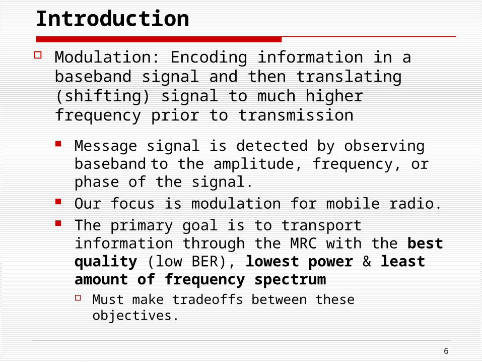
Modulation: Encoding information in a baseband signal and then translating (shifting) signal to much higher frequency prior to transmission

Message signal is detected by observing baseband to the amplitude, frequency, or phase of the signal.

Our focus is modulation for mobile radio. The primary goal is to transport information

through the MRC with the best quality (low BER), lowest power & least amount of frequency spectrum Must make tradeoffs between these objectives.

7

Must overcome difficult impairments introduced by MRC: Fading/multipath Doppler Spread ACI & CCI

Challenging problem of ongoing work that will likely be ongoing for a long time. Since every improvement in modulation methods in

creases the efficiency in the usage of highly scarce spectrum.

8

I. Analog Amplitude and Frequency Modulation

A. Amplitude Modulation

9

10

Spectrum of AM wave

Spectrum of baseband signal. Spectrum of AM wave.

( ) [ ( ) ( )] [ ( ) ( )]2 2

c a cc c c c

A k AS f f f f f M f f M f f

11

B. Frequency Modulation Most widely used form of Angle modulation for

mobile radio applications AMPS Police/Fire/Ambulance Radios

Generally one form of "angle modulation" Creates changes in the time varying phase (angle) of

the signal. Many unique characteristics

12

Unlike AM, the amplitude of the FM carrier is kept constant (constant envelope) & the carrier frequency is varied proportional to the modulating signal m(t) :

fc plus a deviation of kf m(t)

kf : frequency deviation constant (in Hz/V) - defines am

ount magnitude of allowable frequency change

13

(a) Carrier wave.

(b) Sinusoidal modulating signal.

(c) Amplitude-modulated signal.

(d) Frequency-modulated

signal.

14

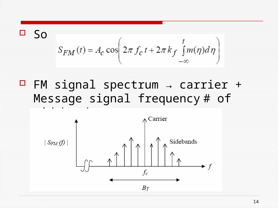
So

FM signal spectrum → carrier + Message signal frequency # of sidebands

15

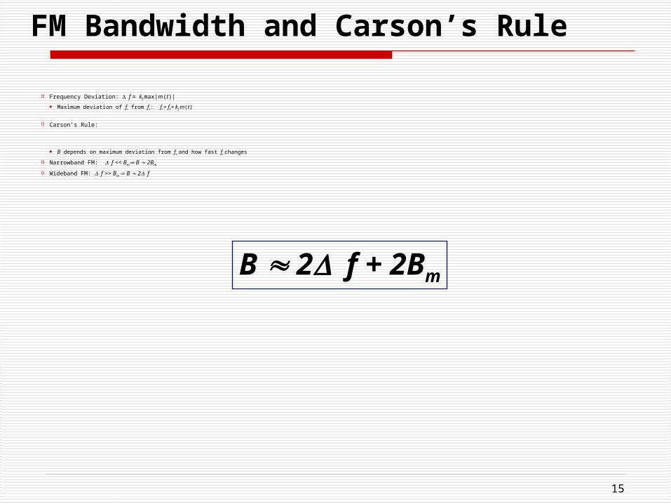
FM Bandwidth and Carson’s Rule

Frequency Deviation: f = kf max|m(t)|

Maximum deviation of fi from fc: fi = fc+ kf m(t)

Carson’s Rule:

B depends on maximum deviation from fc and how fast fi changes

Narrowband FM: f << Bm B 2Bm

Wideband FM: f >> Bm B 2f

B 2f + 2Bm

16

Example: AMPS poor spectral efficiency allocated channel BW = 30 kHz actual standard uses threshold specifications :

17

SNR vs. BW tradeoff in FM one can increase RF BW to improve SNR:

SNRout = SNR after FM detection

≈ ∆f 3SNRin: FM

∆f : peak frequency deviation of Tx the frequency domain

18

rapid non-linear, ∆f 3 improvement in output signal quality (SNRout) for increases in ∆f “capture effect” : FM Rx rejects the weaker of the t

wo FM signals (one with smaller SNRin) in the same

RF BW → resistant to CCI∴ Increased ∆f requires increasing the bandwidth and

spectral occupancy of the signal must exceed the threshold of the FM detector, whic

h means that typically SNRin≥ 10 dB (called the capture threshold)

19

II. Digital Modulation

Better performance and more cost effective than analog modulation methods (AM, FM, etc.)

Used in modern cellular systems Advancements in VLSI, DSP, etc. have made

digital solutions practical and affordable

20

Performance advantages:1) Resistant to noise, fading, & interference

2) Can combine multiple information types (voice, data, & video) in a single transmission channel

3) Improved security (e.g., encryption) → deters phone cloning + eavesdropping

4) Error coding is used to detect/correct transmission errors

5) Signal conditioning can be used to combat hostile MRC environment

6) Can implement mod/dem functions using DSP software (instead of hardware circuits).

21

Choice of digital modulation scheme Many types of digital modulation methods → subtl

e differences Performance factors to consider

1) low Bit Error Rate (BER) at low S/N

2) resistance to interference (ACI & CCI) & multipath fading

3) occupying a minimum amount of BW

4) easy and cheap to implement in mobile unit

5) efficient use of battery power in mobile unit

22

No existing modulation scheme simultaneously satisfies all of these requirements well.

Each one is better in some areas with tradeoffs of being worse in others.

23

Power Efficiency → : ability of a modulation technique to preserve the quality of digital messages at low power levels (low SNR) Specified as Eb / No @ some BER (e.g. 10-5) where Eb : energy/b

it and No : noise power/bit

Tradeoff between fidelity and signal power →

BER ↑ as Eb / No ↓

p

24

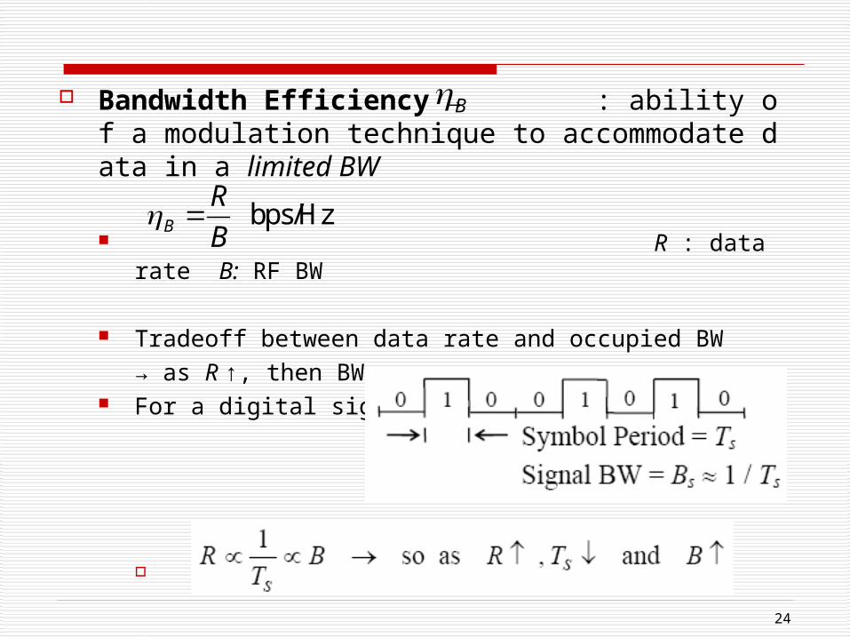
Bandwidth Efficiency → : ability of a modulation technique to accommodate data in a limited BW

R : data rate B: RF BW

Tradeoff between data rate and occupied BW

→ as R ↑, then BW ↑ For a digital signal :

bps/HzB

R

B

B

25

each pulse or “symbol” having m finite states represents n = log2 m bits/symbol → e.g. m = 0 or 1 (2 states) → 1 bit/symbol (binary) e.g. m = 0, 1, 2, 3, 4, 5, 6, or 7 (8 states) → 3

bits/symbol

26

Implementation example: A system is changed from binary to 2-ary. Before: "0" = - 1 Volt, "1" = 1 Volt Now

"0" = - 1 Volt, "1" = - 0.33 volts, "2" = 0.33 Volts, "3" = 1 Volt

What would be the new data rate compared to the old data rate if the symbol period where kept constant?

In general, called M-ary keying

27

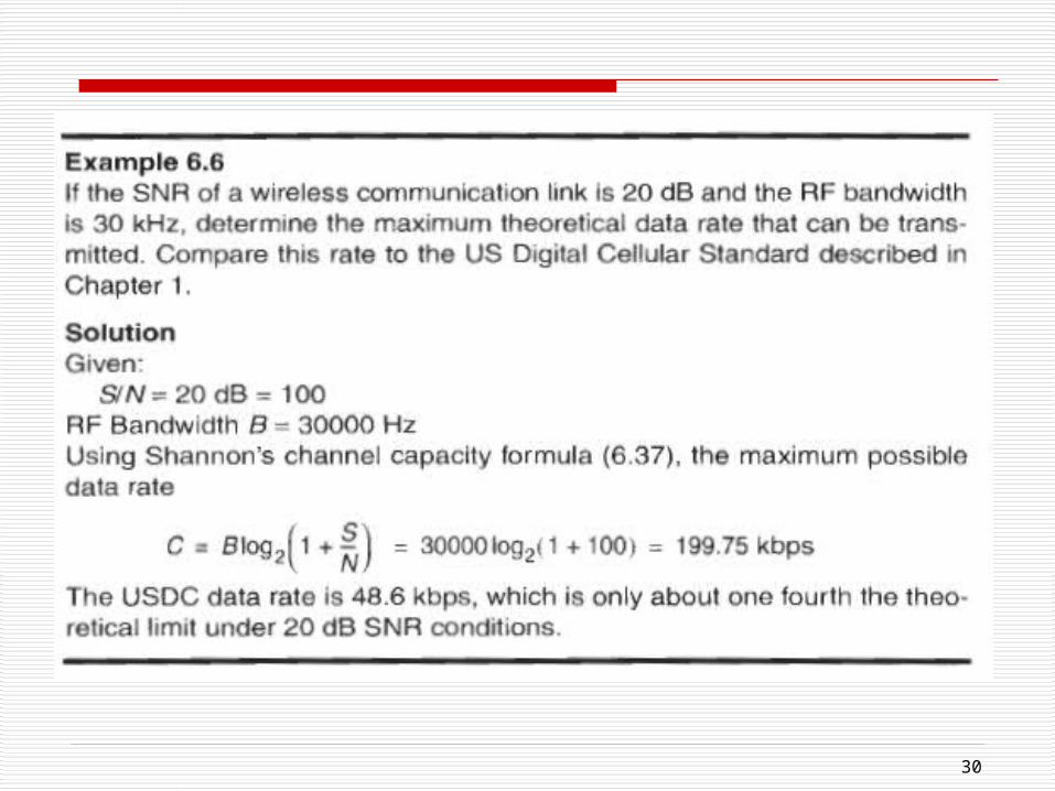
Maximum BW efficiency → Shannon’s Theorem Most famous result in communication theory.

where

B : RF BW C : channel capacity (bps) of real data (not retransmissions

or errors) To produce error-free transmission, some of the bit rate

will be taken up using retransmissions or extra bits for error control purposes.

As noise power N increases, the bit rate would still be the same, but max decreases.

maxB

28

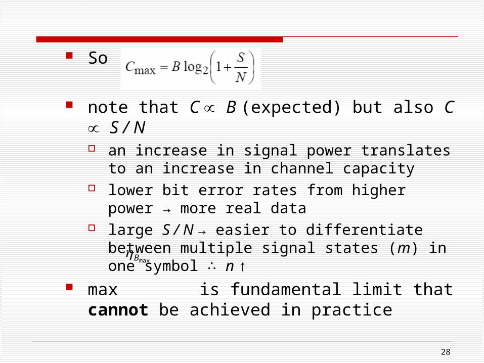
maxB

So

note that C ∝ B (expected) but also C ∝ S / N an increase in signal power translates to an increase in

channel capacity lower bit error rates from higher power → more real

data large S / N → easier to differentiate between multiple

signal states (m) in one symbol ∴ n ↑ max is fundamental limit that cannot be

achieved in practice

29

People try to find schemes that correct for errors.

People are starting to refer to certain types of codes as “capacity approaching codes”, since they say they are getting close to obtaining Cmax. More on this in the chapter on error control.

30

31

32

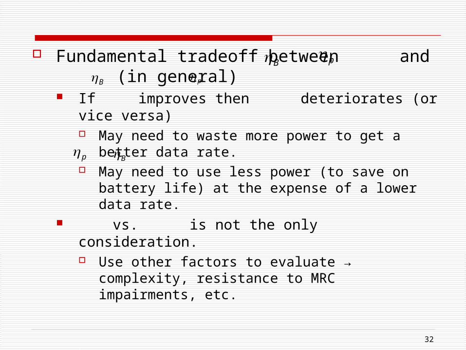
B Fundamental tradeoff between and (in general) If improves then deteriorates (or vice versa)

May need to waste more power to get a better data rate. May need to use less power (to save on battery life) at the

expense of a lower data rate. vs. is not the only consideration.

Use other factors to evaluate → complexity, resistance to MRC impairments, etc.

pB p

Bp

33

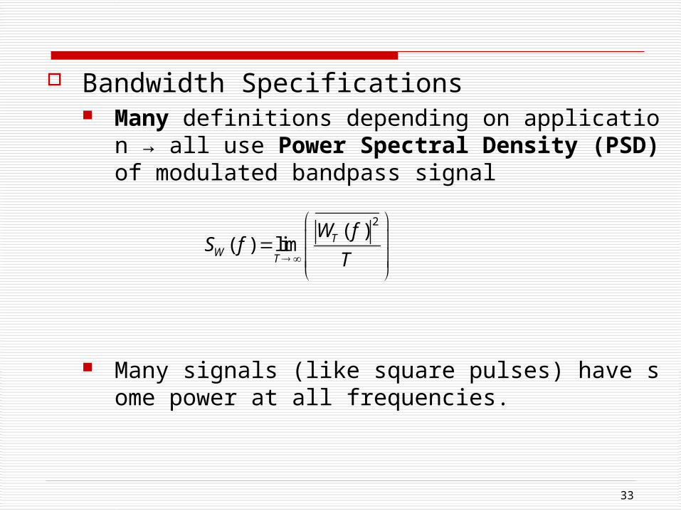
Bandwidth Specifications Many definitions depending on application → all use Powe

r Spectral Density (PSD) of modulated bandpass signal

Many signals (like square pulses) have some power at all frequencies.

2( )

( ) lim TW

T

W fS f

T

34

B’ : half-power (-3 dB) BW B” : null-to-null BW B’” : absolute BW

→ range where PSD > 0 FCC definition of occupied BW → BW contains 99

% of signal power

35

III. Geometric Representation of Modulation Signal

Geometric Representation of Modulation Signals - Constellation Diagrams

Graphical representation of complex ( A & θ) digital modulation types Provide insight into modulation performance

Modulation set, S, with M possible signals

Binary modulation → M = 2 → each signal = 1 bit of information

M-ary modulation → M > 2 → each signal > 1 bit of information

36

Example: Binary Phase Shift Keying (BPSK)

37

Phase change between bits → Phase shifts of 180° for each bit.

Note that this can also be viewed as AM with +/- amplitude changes

Dimension of the vector space is the # of basis signals required to represent S.

38

Plot amplitude & phase of S in vector space :

39

Constellation diagram properties :1) Distance between signals is related to differences in

modulation waveforms Large distance → “sparse” → easy to discriminate → g

ood BER @ low SNR (Eb / No )

From above, noise of -2 added to would make t

he received signal look like s2(t) → error.

From , noise of > - would make the result clos

er to - and would make the decoder choose s2(t)

→ error.

∴ Above example is Power Efficient (related to density

with respect to # states/N)

40

2) Occupied BW ↓ as # signal states ↑ If we can represent more bits per symbol, then we n

eed less BW for a given data rate. Small separation → “dense” → more signal states/s

ymbol → more information/Hz !!

∴ Bandwidth Efficient

41

IV. Linear Modulation Methods

In linear modulation techniques, the amplitude of the transmitted signal varies linearly with the modulating digital signal.

Performance is evaluated with respect to Eb / No

42

BPSK

BPSK → Binary Phase Shift Keying

43

Phase transitions force carrier amplitude to change from “+” to “−”. Amplitude varies in time

44

BPSK RF signal BW

Null-to-null RF BW = 2 Rb = 2 / Tb

90% BW = 1.6 Rb for rectangular pulses

45

Probability of Bit Error is proportional to the distance between the closest points in the constellation. A simple upper bound can be found using the

assumption that noise is additive, white, and Gaussian.

d is distance between nearest constellation points.

46

Q(x) is the Q-function, the area under a normalized Gaussian function (also called a Normal curve or a bell curve)

Appendix F, Fig. F.1 Fig. F.2, plot of Q-function Tabulated values in Table F.1.

Here

dyezQ y

z

2/2

2

1)(

47

Demodulation in Rx Requires reference of Tx signal in order to properly d

etermine phase carrier must be transmitted along with signal

Called Synchronous or “Coherent” detection complex & costly Rx circuitry good BER performance for low SNR → power efficient

48

49

DPSK

DPSK → Differential Phase Shift Keying Non-coherent Rx can be used

easy & cheap to build no need for coherent reference signal from Tx

Bit information determined by transition between two phase states incoming bit = 1 → signal phase stays the same as prev

ious bit incoming bit = 0 → phase switches state

50

If {mk} is the message, the output {dk} is as shown below.

can also be described in modulo-2 arithmetic

Same BW properties as BPSK, uses same amount of spectrum

Non-coherent detection → all that is needed is to compare phas

es between successive bits, not in reference to a Tx phase.

power efficiency is 3 dB worse than coherent BPSK (higher po

wer in Eb / No is required for the same BER)

1k k kd m d

51

52

QPSK

QPSK → Quadrature Phase Shift Keying

Four different phase states in one symbol period Two bits of information in each symbol

Phase: 0 π/2 π 3π/2 → possible phase values

Symbol: 00 01 11 10

53

Note that we choose binary representations so an error between two adjacent points in the constellation only results in a single bit error

For example, decoding a phase to be π instead of π/2 will result in a "11" when it should have been "01", only one bit in error.

54

Constant amplitude with four different phases remembering the trig. identity

55

56

Now we have two basis functions Es = 2 Eb since 2 bits are transmitted per symbol

I = in-phase component from sI(t).

Q = quadrature component that is sQ(t).

57

QPSK RF Signal BW

null-to-null RF BW = Rb = 2RS (2 bits / one symbol time) = 2 / Ts double the BW efficiency of BPSK → or twice the data rate in same si

gnal BW

58

BER is once again related to the distance between constellation points.

d is distance between nearest constellation points.

59

60

How does BER performance compare to BPSK?

Why? same # of states per number of basis functions for both BPSK and QPSK (2 states per one function or 4 states per 2 functions)

same power efficiency

(same BER at specified Eb / No) twice the bandwidth efficiency

(sending 2 bits instead of 1)

61

QPSK Transmission and Detection Techniques

62

63

OQPSK

Offset QPSK The occasional phase shift of π radians can cause the

signal envelope to pass through zero for just in instant.

Any kind of hard limiting or nonlinear amplification of the zero-crossings brings back the filtered sidelobes since the fidelity of the signal at small voltage levels is l

ost in transmission. OQPSK ensures there are fewer baseband signal tran

sitions applied to the RF amplifier, helps eliminate spectrum regrowth after amplification.

64

Example above: First symbol (00) at 0º, and the next symbol (11) is at 180º. Notice the signal going through zero at 2 microseconds. This causes problems.

65

Using an offset approach: First symbol (00) at 0º, then an intermediate symbol at (10) at 90º, then the next full symbol (11) at 180º. The intermediate symbol is used halfway through

the symbol period. It corresponds to allowing the first bit of the symbol

to change halfway through the symbol period. The figure below does have phase changes more

often, but no extra transitions through zero. IS-95 uses OQPSK, so it is one of the major

modulation schemes used.

66

67

In QPSK signaling, the bit transitions of the even and odd bit streams occur at the same time instants.

but in OQPSK signaling, the even and odd bit Streams, mI(t) and mQ(t), are offset in their relative alignment by one bit period (half-symbol period)

68

the maximum phase shift of the transmitted signal at any given time is limited to ± 90o

69

The spectrum of an OQPSK signal is identical to that of a QPSK signal, hence both signals occupy the same bandwidth

70

π/4 QPSK

π/4 QPSK The π/4 shifted QPSK modulation is a quadrature ph

ase shift keying technique offers a compromise between OQPSK and QPSK in ter

ms of the allowed maximum phase transitions. It may be demodulated in a coherent or noncoheren

t fashion. greatly simplifies receiver design.

In π/4 QPSK, the maximum phase change is limited to ± 135o

in the presence of multipath spread and fading, π/4 QPSK performs better than OQPSK

71

72

73