1

Multiple Kernel Multiple Kernel LearningLearning

Naouel BailiMRL Seminar, Fall 2009

2

Introduction

Multiple Kernel Learning (MKL) Given M kernel functions K1,...,KM that are potentially well suited for a given problem, find a positive combination of these kernels such that the resulting kernel K is « optimal » in some sence,

Need to learn together the kernel coefficients

dm and the SVM parameters

3

State of the art [Lanckriet et al., 04]: Semi-definite programming [Bach et al., 04]: SMO [Sonnenburg et al., 06]: Semi-infinite linear

programming [Rakotomamonjy et al., 08]: Gradient descent,

simpleMKL [Chapellel et al., 02]: Gradient descent for general kernel [Chapellel et al., 08]: Second order optimization of

kernel parameters

All solve the same problem, but use different optimization techniques. SimpleMKL has been shown to be more efficient.

The last method presents a Newton type optimization technique for MKL which turns out to be even more efficient than simpleMKL.

4

Gradient descent, simpleMKL

Rakotomamonjy et al., 08

5

MKL Primal problem

In the MKL framework, we look for decision function of the form where each function fm belongs to a different RKHS Hm associated with a kernel Km. Inspired by the multiple smoothing splines framework of [Wahba, 90], we propose to address the MKL SVM problem by solving the following convex problem:

6

MKL Dual problem

We take the Langragian of the primal problem and set its gradient to zero with respect to the primal variables. Plugging the obtained optimatily conditions in the Lagragian gives the dual problem:

7

Objective function

We consider the following constrained optimization problem:

By setting to zero the derivatives of the Lagrangian according to the primal variables, we derive the associated dual problem:

8

Optimal SVM value and its derivatives

Because of stron duality, J(d) is the objective value of the dual problem:

J(d) can be obtained by any SVM algorithm. Thus, the overall complexity of SimpleMKL is tied to the one of the single kernel SVM algorithm.

We assume that each Gram matrix is positive definite, with all eigenvalues greater than some η>0. It implies that, for any admissible d, the dual problem is strictly concave. The strict concavity property ensures that α* is unique. Furthermore, the derivatives of J(d) can be computed as if α* were not to depend on d:

9

Search direction With the positivity assumption on the kernel

matrices, J(.) is convex and differentiable with Lipshitz gradient. The approach we use for solving this problem is the reduced gradient method, which converges for such functions.

One the gradient of J(d) is computed, d is updated by using a descent direction ensuring that equality constraints and the non-negativity on d are satisfied:

10

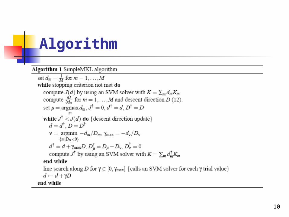
Algorithm

11

Optimality conditions From the primal and dual objectives, the MKL duality

gap is:

If J(d*) has been obtained through the dual problem, then this MKL duality gap can also be computed from the single SVM algorithm duality gap:

Then the MKL duality gap becomes:

12

Experiments (1)

Comparison with SILP on several UCI datasets. Kernels are centered and normalized to unit trace.

Evaluation of the three largest weights dm for SimpleMKL and SILP:

13

Experiments (2)

Average performance measures for SILP, SimpleMKL and a plain gradient descent algorithm:

14

Conclusion

SimpleMKL framework results in a smooth and convex optimization problem

The main added value of the smoothness of the objective function is that descent methods become practical and efficient means to solve the optimization problem that wraps a single kernel SVM solver

SimpleMKL is significantly more efficient that the state-of-the art SILP approach.

15

Second order optimization of kernel

parameters

Chapellel et al., 08

16

Objective function

Consider a hard margin SVM with a kernel K. The following objective function is maximized:

Since finding the maximum margin solution seems to give good empirical results, it has been proposed to extend this idea for MKL: find the kernel that maximizes the margin or equivalently

17

Problem The SVM objective function has been derived

for finding an hyperplane for a given kernel, not for learning the kernel matrix.

Illustration of the problem: since Ω(dK) = Ω(K)/d, can be trivially minimized.

This is usually fixed by adding the constraint ∑dm ≤ 1. But is the L1 norm on d the most appropriate?

18

Hypermarameter view

A more principle approach is to consider the dm as hyperparameters and tune them on a model selection criterion. A convenient criterion is a bound on the generalization error [Bousquet, Herrmann, 03], T(K)Ω(K), where T(K) is the re-centered trace,

Because Ω(dK) = Ω(K)/d, this is equivalent to minimize Ω(K) under constraint T(K) = constant, or

19

Optimization

No need for complex optimization techniques. Simply define:

and perform a gradient based optimization of J which is twice differentiable almost everywhere.

For a given d, let α* be the SVM solution.

20

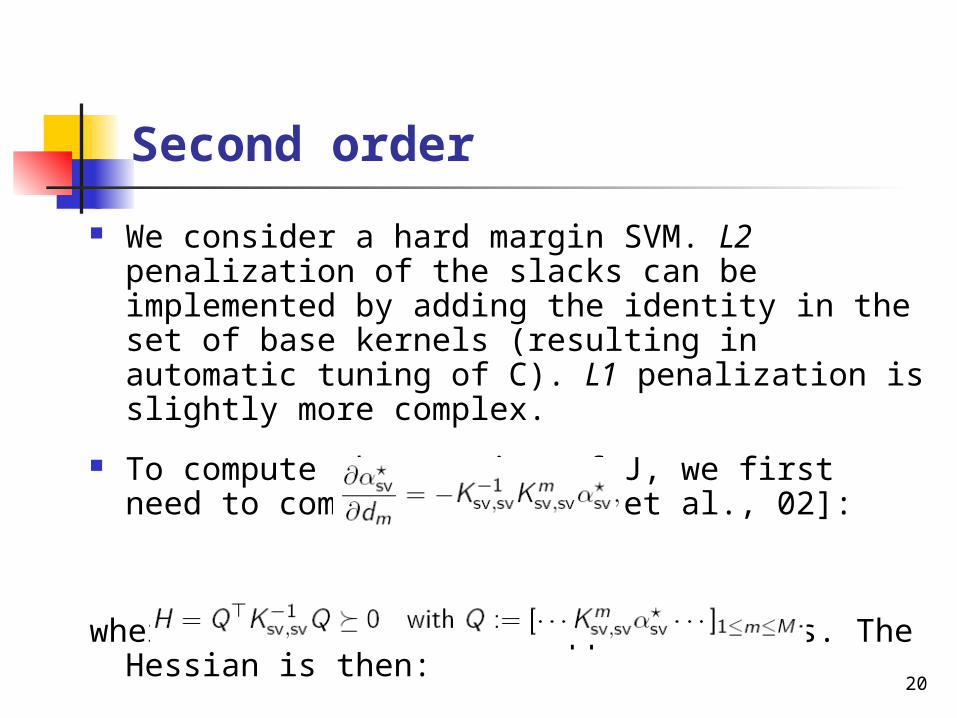
Second order

We consider a hard margin SVM. L2 penalization of the slacks can be implemented by adding the identity in the set of base kernels (resulting in automatic tuning of C). L1 penalization is slightly more complex.

To compute the Hessian of J, we first need to compute [Chapelle et al., 02]:

where sv is the set of support vectors. The Hessian is then:

21

Search direction

The step direction s is a constrained Newton step found by minimizing the quadratic problem:

The quadratic form corresponds to the second order expansion of J.

The constraints ensure that any solution on the segment [d; d+s] satisfies the original constraints.

Finally backtracking is performed in case J(d + s) ≥ J(d).

22

Complexity

For each iteration: SVM training: Inverting Ksv;sv is , but might already be

available as a by-product of the SVM training. Computing H: Finding s:

The number of iterations is usually less than 10.

When M < nsv, computing s is not more expensive than the SVM training.

23

Experiments (1)

Comparison with simpleMKL on several UCI datasets as in [Rakotomamonjy et al., 08] Kernels are centered and normalized.

Relative duality gap as a function of the number of iterations:

24

Experiments (2)

Example of convergence behavior of the weights dm on Ionosphere:

25

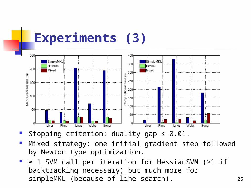
Experiments (3)

Stopping criterion: duality gap ≤ 0.01. Mixed strategy: one initial gradient step followed by

Newton type optimization. ≈ 1 SVM call per iteration for HessianSVM (>1 if

backtracking necessary) but much more for simpleMKL (because of line search).

26

Conclusion

Simple optimization strategy for MKL: requires just standard SVM training and small QP (whose size is the number of kernels).

Very fast method because: The number of SVM trainings is small (of the order of

10) The extra cost required for computing the Newton type

direction is not prohibitive. As an aside, MKL should be considered as a

model selection problem. From this point of view, need for centering and normalizing the kernel matrices.