1 Outline.

1. (Quick) Review of OLS Theory

2. Where do regressions come from?

3. Alternatives to OLS

4. GLS, Weighting and Standard Errors

5. Misspecification

6. IV (next week)

2 Review of OLS Theory

• The theory of ols is summarized in this chapter.

• Fortunately, you have seen it before in detail.

• The assumptions that are made in the text are:

1. The data generating process is y = Xβ + u

2. Data are independent over i with E[u|X] = 0

and E£uu0

¤= Ω = Diag[σ2i ]

3. The Matrix X is full rank

4. plim 1NX0X =Mxx exists and is finite nonsingular

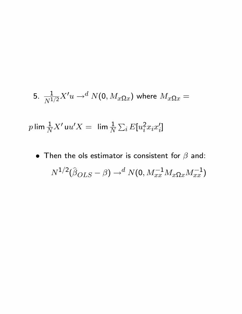
5. 1N1/2X

0u→d N(0,MxΩx) where MxΩx =

p lim 1NX 0 uu0X = lim 1

N

Pi E[u

2i xix

0i]

• Then the ols estimator is consistent for β and:

N1/2(bβOLS − β)→d N(0,M−1xx MxΩxM

−1xx )

3 Where do regressions come from?

• In this chapter, we study the classic linear regres-sion model.

yi = x0iβ + εi

• y is dependent variable, x is a set of regressors

and ε are error terms

• In practice, it can be difficult to specify y, x andε.

• In this section, we ask where these regressionsmight come from.

• Familiarity with much of the theory of ols will beassumed.

3.1 Data Description

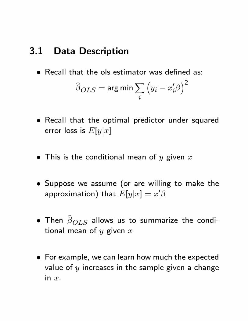
• Recall that the ols estimator was defined as:bβOLS = argminX

i

³yi − x0iβ

´2

• Recall that the optimal predictor under squarederror loss is E[y|x]

• This is the conditional mean of y given x

• Suppose we assume (or are willing to make theapproximation) that E[y|x] = x0β

• Then bβOLS allows us to summarize the condi-

tional mean of y given x

• For example, we can learn how much the expectedvalue of y increases in the sample given a change

in x.

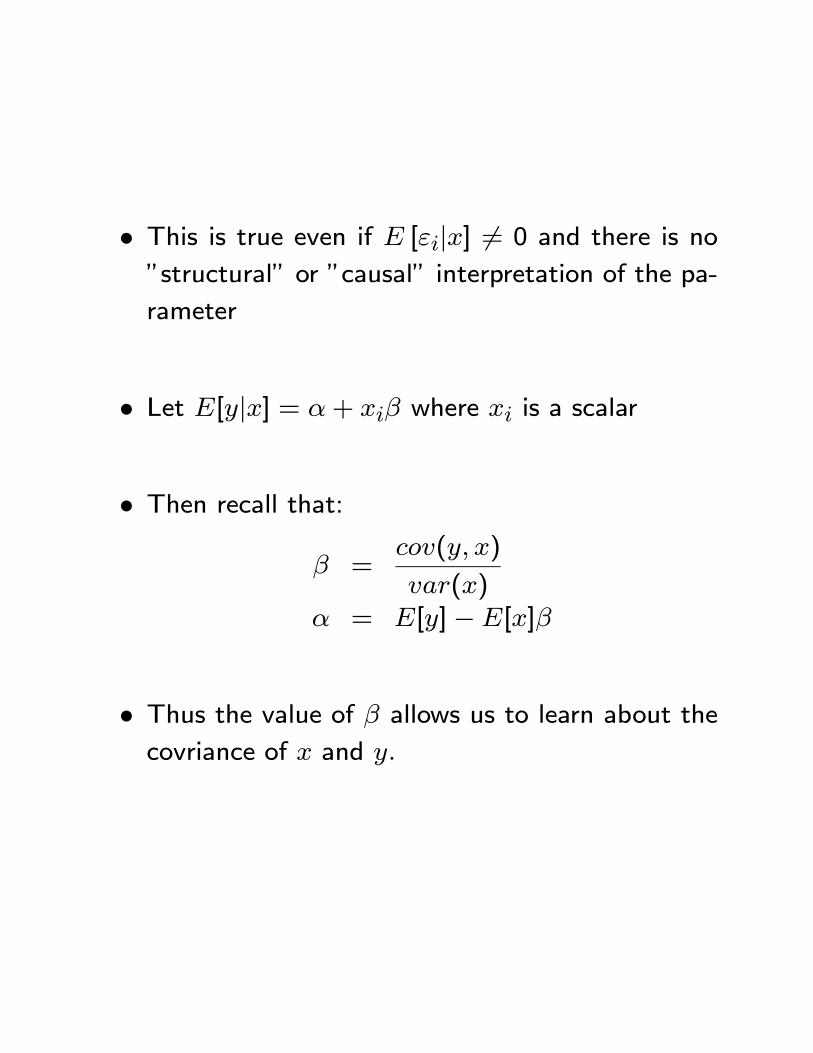
• This is true even if E [εi|x] 6= 0 and there is no

”structural” or ”causal” interpretation of the pa-

rameter

• Let E[y|x] = α+ xiβ where xi is a scalar

• Then recall that:

β =cov(y, x)

var(x)α = E[y]−E[x]β

• Thus the value of β allows us to learn about thecovriance of x and y.

3.2 Potential Outcome Model

• A second case that may generate a regression isif:

yi = αi + βix+ γDi + εi

• Here Di is a ”treatment” which usually takes on

values 0,1

• x are exogenous variables (e.g. demographics)

• Example 1: Marketers engage in advertising ex-periments to learn the elasticity of expenditure

with respect to promotions

• Example 2: Development economists assign bonuspayments (at random) to teachers to show up to

work to learn about the effectiveness of incentives

to improve teacher attendance.

• If the assumptions of ols hold, most importantlyE[εi|x,Di] = 0 then we can get an estimate of

the ”causal” effect Di

• In many applications, however, Di will be cor-

related with εi (e.g. schooling correlated with

unobserved ability).

3.3 Reduced form models

• One classical example is a hedonic regression.

• In this setting i is a good in a differentiated prod-uct market

• The dependent variable is pi, the price of good i

• xi are the characteristics of good i (e.g. if the

market is housing, square footage, lot size, neigh-

borhood characteristics, etc...)

• The error term εi is thought to be measurement

error in price or an omitted product characteristic.

• Assume that consumers are utility maximizing,e.g. the choose i :

maxi

u(xi, y − pi)

• Consumers get a flow of utility from xi and a

composite commodity c = y − pi

• If we allow for strict monotonicity in utility, we canprove that equilibrium prices must be a function

of characterstics (and characteritics only):

pi = xiβ + εi

• This is a reduced form since we are not uncoveringthe primitive supply and demand parameters.

• Note however, that β gives us the MRS betweenxi and the composite commodity

• Housing hedonics are widely used since they allowus to get a willingness to pay measure for school

quality, environmental amentities by estimating β

• Hedonics are used by the Bureau of Labor statis-tics to do ”quality adjustments” required to com-

pute inflation.

• Hedonics are used in eBay data to price the valueof a good reputation.

• Big assumption: E[εi|x] = 0.

• Omitted attributes are independent of observedattributes.

• A second example is dynamic programming.

• The theory in Stokey-Lucas implies that the solu-tion to dynamic stochastic control problems can

be written as a stationary function of the state

variables in many settings.

• For instance, in a standard model of the firm,investment is the dependent variable.

• The state might include capital, input prices, de-mand shocks, productivity shocks etc...

• This could motivate an ols regression of the re-duced form investment function as:

log(investment) = α0+β1capital+β2input price+....+εi

• What is εi?

• Mathematically, εi is the influence of all factorsthat we did not include as a regressor

• These include omitted state variables and mea-surement error in investment.

• Exogeneity may be controversial.

• For instance, εi may be thought of as includingproductivity.

• We would expect productivity to be correlatedwith capital and possibly other states.

3.4 Structural Models

• A first example is production function estimation.

• Here i denotes a firm

• Here the dependent variable is a measure of out-put (e.g. value added)

• The independent variables are capital and labor

• The error term is a productivity residual

• We usually use a log-linear specification since valueadded is not typically negative in the data.

yi = α+ βlli + βkki + ωi

• The coefficients and error term characterize a firm’stechnology.

• Obviously, E[ωi|li, ki] = 0 will be controversial

• Theory suggests that more productive firms willuse more labor.

• There may be a negative correlation between k

and ω because firms with a large capital stock

may be able to ”ride out” bad productivity shocks

and avoid exit.

• A second example is empirical auctions.

• Consider a first price sealed bid auction, such ascontractors bidding for bridge/highway jobs.

• The dependent variable is firm i’s bid.

• The control variables are a set of project charac-teritics.

• Following the theory of Bayes-Nash equilibrium,assume that costs can be written as:

ci,t = x0i,tβ + ξi + ξt + ηi,t

• ci,t cost for firm i in project t

• xi,t observed cost controls (e.g. distance to project,

engineering cost estimate)

• ξi firm i fixed effect

• ξt project t fixed effect

• ηi,t independent shock to costs

• Let Q(bi,t|xi,t, ξ) be the probability that a bid ofbi,t wins given the info that is publically observed

to firms

• Let bQ(bi,t|xi,t, ξ) be an estimate of this objectand bq(bi,t|xi,t, ξ) an estimate of the associateddensity

• For instance, we could specify a distribution forQ and use MLE conditioning on x and ξ.

• We shall dicuss general methods for doing this ina later chapter.

• Then the firm’s profit max problem is:

(bi,t − ci,t)Q(bi,t|xi,t, ξ)

• The FOC’s for profit maximization are:

Q(bi,t|xi,t, ξ) + (bi,t − ci,t)q(bi,t|xi,t, ξ) = 0

• Algebra implies that

bi,t = ci,t +Q(bi,t|xi,t, ξ)q(bi,t|xi,t, ξ)

= x0i,tβ + ξi + ξt +bQ(bi,t|xi,t, ξ)bq(bi,t|xi,t, ξ) + ηi,t

• In the second step we replace Q(bi,t|xi,t,ξ)q(bi,t|xi,t,ξ) with its

sample analogue

• Exogeneity means that E[ηi,t|xi,t, ξ] = 0

• A few things to note:

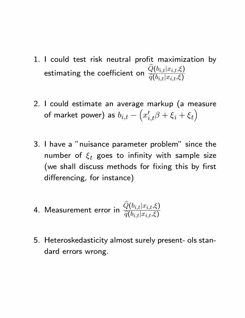
1. I could test risk neutral profit maximization by

estimating the coefficient onbQ(bi,t|xi,t,ξ)bq(bi,t|xi,t,ξ)

2. I could estimate an average markup (a measure

of market power) as bi,t −³x0i,tβ + ξi + ξt

´

3. I have a ”nuisance parameter problem” since the

number of ξt goes to infinity with sample size

(we shall discuss methods for fixing this by first

differencing, for instance)

4. Measurement error inbQ(bi,t|xi,t,ξ)bq(bi,t|xi,t,ξ)

5. Heteroskedasticity almost surely present- ols stan-

dard errors wrong.

4 Alternatives to OLS

• OLS is based on a quadratic loss function.

• Why mimimize a quadratic loss function?

• We shown, theoretically that under some assump-tions (e.g. homoskedasticity) OLS can be effi-

cienct.

• However, quadratic loss has some disadvantages.

• First, there may be sensitivity to outliers (remem-ber, we are squaring).

• In general, we will want to plot fitted residualsto see if our results are driven by a handful of

observations.

• Also, the loss function may not be related to de-cision making.

• Bayes takes into account the later.

• This can be important in some applications, e.g.global warming.

• Another important set of loss functions is basedon an absolute value norm.

• Claim: The minimizer of the loss function belowis the median: X

i:yi≥β|yi − β|

• Intuition. Suppose we have 9 observations.

• The median is the 5th observation, suppose it is10 and the 6th observation is 12.

• If we set β = 12, we add 2 to observations 1-5

and subtract 2 from observations 6-9.

• The 6th observation cannot be minimizing.

• By symmetry, neither can the 4th.

• A nice feature of the median is that it is less sen-stive to outliers.

• More generally, we are interested in the qth quan-tile.

• This is the solution to the following minimizationproblem:X

i:yi≥βq |yi − β|+

Xi:yi<β

(1− q) |yi − β|

• The qth quantile regression estimator is:Xi:yi≥x0iβ

q¯yi − x0iβq

¯+

Xi:yi<x

0iβ

(1− q)¯yi − x0iβq

¯

• This will give us the qth quantile conditional onthe regressors x.

• An advantage of quantile estimation is that weget a different value of β for every value of q.

• This allows us to capture heterogeneity in condi-tional means/casual effects and so forth.

• Figure 4.1 shows that regression models may missa lot.

5 GLS, Weighting and Standard Er-

rors

• In general, with heteroskedastic error terms, olsis not efficient.

• However, we can get back to efficiency by dividingthrough by 1

σiin a heteroskedastic model.

• That is, we transform the variables as:

1

σiyi =

1

σi

³x0iβ + εi

´y∗i = x∗i + ε∗i

• Note that V ar[ε∗i ] = V ar[ 1σiεi] =

1σ2iσ2i = 1

• Hence, we are back to homoskedasticity.

• Hence, ols using (y∗i , x∗i ) is efficient.

• The intuition is that we should underweight ob-servations with high variance and overweight ob-

servations with low variance.

• The GLS estimator is:

bβGLS = ³X 0Ω−1X

´−1X 0Ω−1y

• In practice, we do not know Ω−1.

• A Feasible GLS (FGLS) estimator comes up withan estimate bΩ−1 and then:

bβFGLS = ³X 0 bΩ−1X´−1X 0 bΩ−1y

• Big Practical Problem: How to estimate bΩ−1?

• Normally we need to make a strong functionalform assumption such as σi = σx

• If we misspecify this functional form, our standarderrors for FGLS will be wrong!

• FGLS may be worse than OLS.

• Probably the most commonly used alternative inpractice for computing standard errors is Robust

standard errors proposed by White.

• Recall that

N1/2³bβOLS − β

´=

µ1

NX 0X

¶−1N−1/2X0u

bβOLS − β =µ1

NX 0X

¶−1 1NX0u

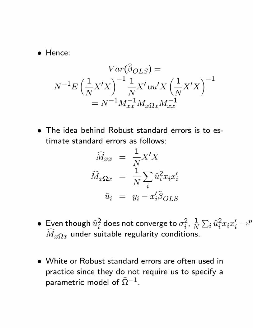
• Hence:

V ar(bβOLS) =N−1E

µ1

NX 0X

¶−1 1NX0 uu0X

µ1

NX 0X

¶−1= N−1M−1

xx MxΩxM−1xx

• The idea behind Robust standard errors is to es-timate standard errors as follows:

cMxx =1

NX 0X

cMxΩx =1

N

Xi

bu2i xix0ibui = yi − x0ibβOLS

• Even though bu2i does not converge to σ2i , 1N Pi bu2i xix0i→pcMxΩx under suitable regularity conditions.

• White or Robust standard errors are often used inpractice since they do not require us to specify a

parametric model of bΩ−1.

• Bottom line: most practioners, when estimating

a regression using cross sectional data will use ols

combined with robust standard errors.

• In STATA, regress y x cluster (id) robust

• Also, it is common to cluster the standard errors(we will discuss this in a late chapter).

• FGLS is not very commonly used.

• Finally, suppose you have a variable xi that youbelieve is proportional to σi

• For example, in a production function regression,we may conjecture that the variance of ωi may

be proportional to ki

• Aitkin’s theorem suggests that we may want to

weight the observations by 1ki

• This may generate a more efficient estimator.

6 Misspecification

• Next we consider various ways in which our modelmay be misspecified and its consequences.

6.1 Functional Form

• Suppose that the true functional form is non-

linear

y = g(x) + v

• where g(x) is some general, nonlinear function

• It can be shown (not surprisingly) that ols mini-mizes the following mean square prediction error:

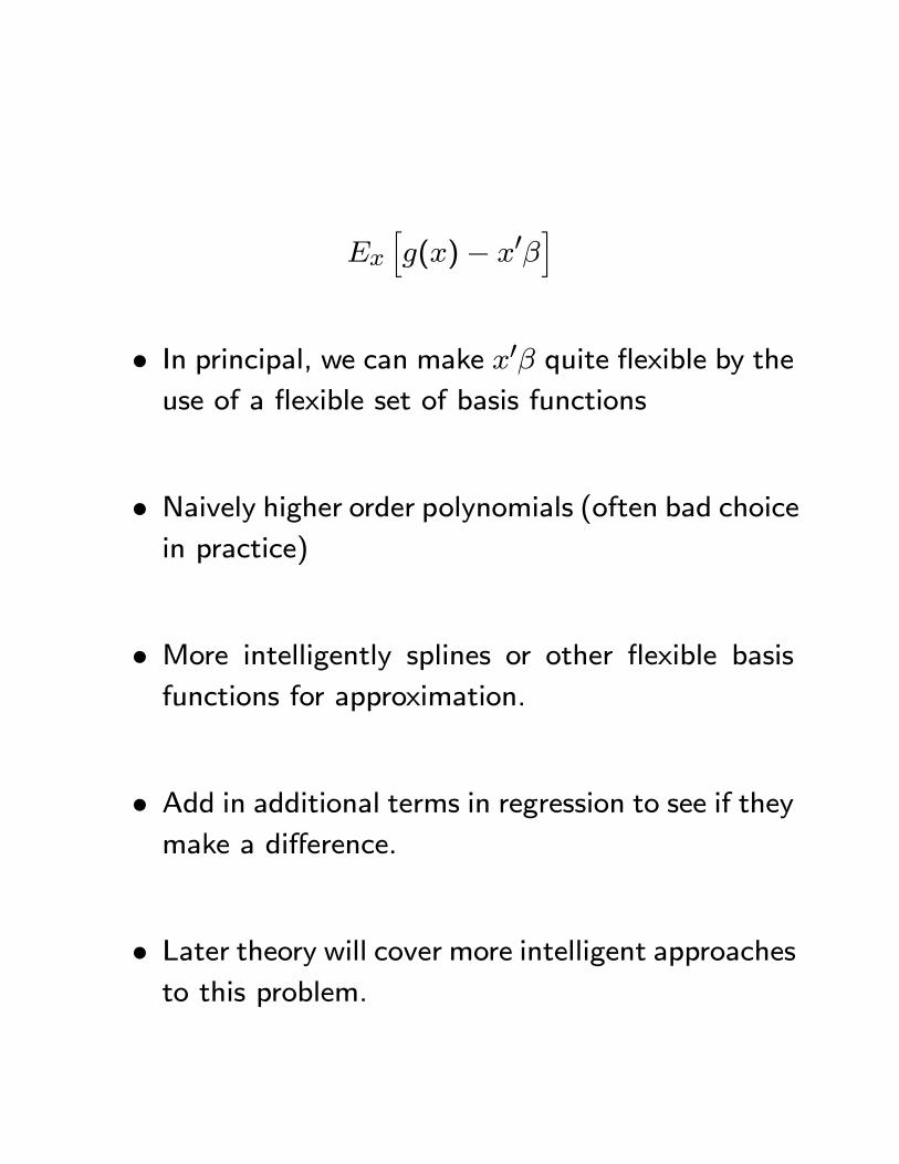
Ex

hg(x)− x0β

i

• In principal, we can make x0β quite flexible by theuse of a flexible set of basis functions

• Naively higher order polynomials (often bad choicein practice)

• More intelligently splines or other flexible basisfunctions for approximation.

• Add in additional terms in regression to see if theymake a difference.

• Later theory will cover more intelligent approachesto this problem.

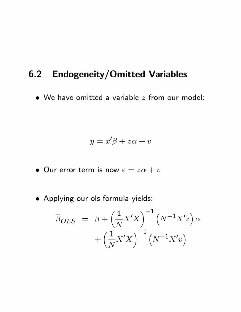
6.2 Endogeneity/Omitted Variables

• We have omitted a variable z from our model:

y = x0β + zα+ v

• Our error term is now ε = zα+ v

• Applying our ols formula yields:

bβOLS = β +µ1

NX0X

¶−1 ³N−1X 0z

´α

+µ1

NX 0X

¶−1 ³N−1X0v

´

• If we assume E [v|x] = 0 then:

p lim bβOLS = β + p limµ1

NX 0X

¶−1 ³N−1X0z

´α

= β + δα

δ = p limµ1

NX0X

¶−1 ³N−1X 0z

´

• If our omitted variable is highly correlated with z,³N−1X0z

´will be large and so will δ.

• Thus the x proxies for both the effect of the x’sdirectly and also for the effect of the z.

• In the limit, bβOLS converges in probability to its”psuedo true value” β + δα