1

Overview of Experimental Design

2

3

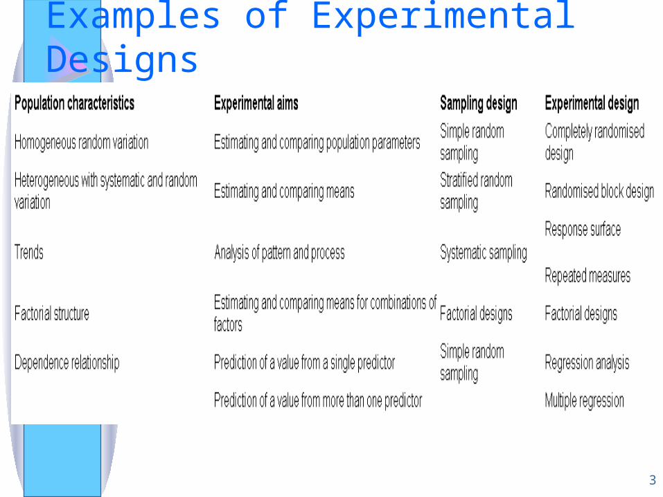
Examples of Experimental Designs

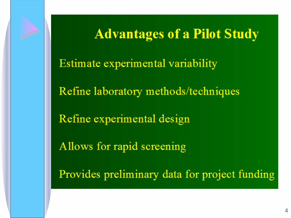
4

5

Basic Experimental Design Tests

6

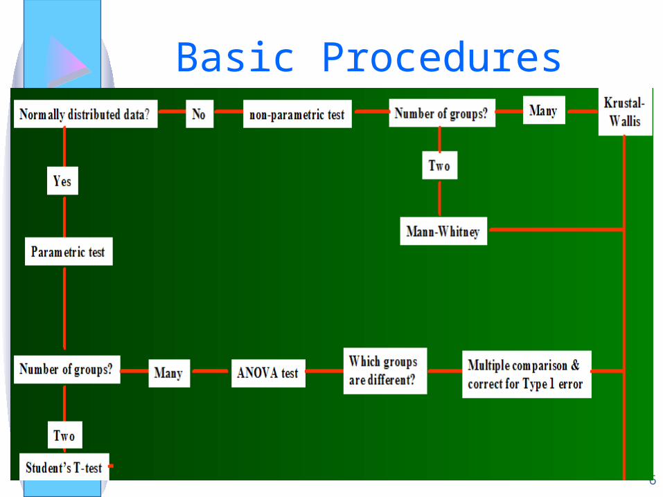
Basic Procedures

7

8

Definition of Factor• Don’t confuse Factor in Principal Component Factor

Analysis with Factor in Experimental Design. • Factors are related to treatments. Treatments have

levels. For example, a treatment could be time that it takes to complete a task. Time could be categorized into 3 time intervals.

• Blocks are also treatments or factors. However, the term block is used to indicate a factor that is not of primary interest. Blocks help to explain variation in the data.

• The term treatment combinations means that various treatment levels are selected.

9

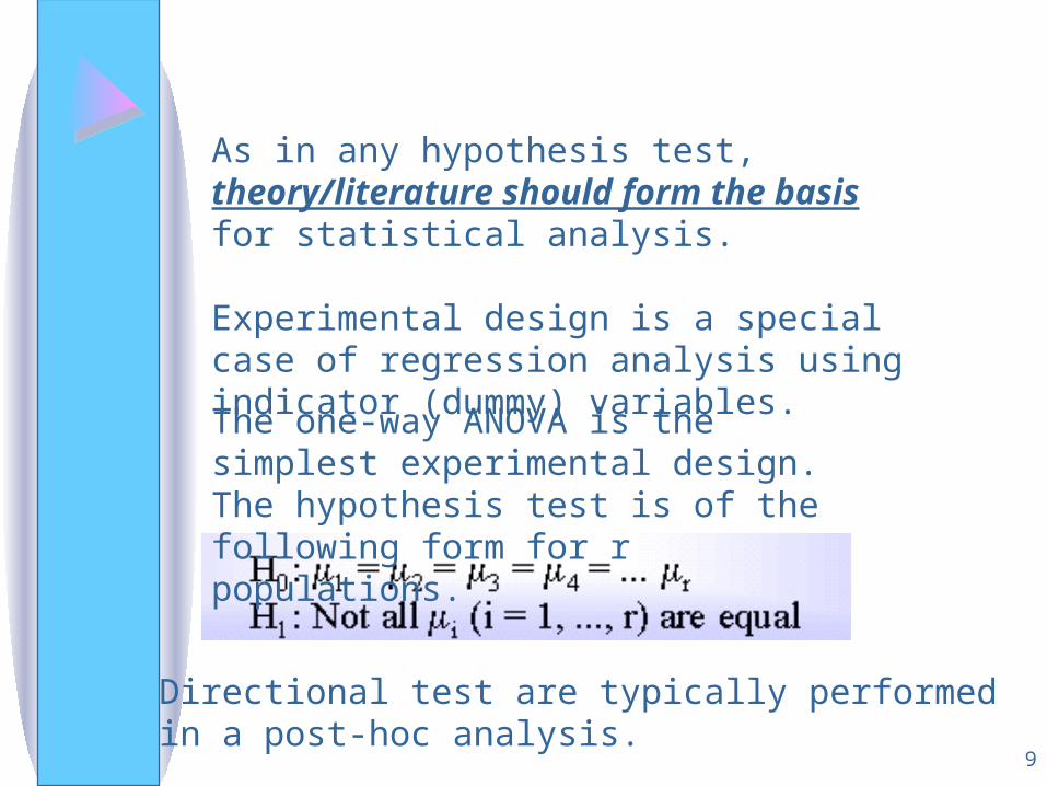
As in any hypothesis test, theory/literature should form the basis for statistical analysis.

Experimental design is a special case of regression analysis using indicator (dummy) variables.

The one-way ANOVA is the simplest experimental design. The hypothesis test is of the following form for r populations.

Directional test are typically performed in a post-hoc analysis.

10

Basic Principle of One-Way ANOVA

• When the population means are not equal, the “average” error (within sample) is relatively small compared with the “average” treatment (between sample deviation).

• F = (f(error effects) + f(treatment effects)) /f(error effects),

where f( ) is a function and F is the test statistic.

11

The procedure for selecting sample data with the independent variables set in advance is called a design of the experiment. The statistical procedure for comparing the population means is called an analysis of variance.

Definition 1The process of collecting sample data is called an experiment

Definition 2The plan for collecting the sample is called the design of the experiment

Definition 3The variable measured in the experiment is called the response variable.

12

Definition 4The object upon which the response y is measured is called an experimental unit.

Definition 5The independent variables, quantitative or qualitative, that are related to a response variable y are called factors.

Definition 6The intensity setting of a factor (i.e., the value assumed by a factor in an experiment) is called a level.

Definition.7A treatment can be thought of as a particular combination of levels of the factors involved in an experiment.

13

A designed experiment. A marketing study is conducted to investigate the effects of brand and shelf location on weekly coffee sales. Coffee sales are recorded for each of two brands (brand A and brand B) at each of three shelf locations (bottom, middle, and top). The 2 x 3 = 6 combinations of brand and shelf location were varied each week.

14

Week 1 9 14

Week 2 7 16

Week 4 12 17

Week 5 10 13

Week 3 8 18

Week 6 11 15

A

B

SHELF LOCATIONBottom Middle Top

Brands

15

A. Since the data will be collected each week, experimental unit is the store shelves each week.

B. The variable of interest, i.e. the response, is y = weekly coffee sales. Note that weekly coffee sales is a quantitative variable.

16

C. Since we are interested in investigating the effect of brand and shelf location on sales, brand and shelf location are the factors. Note that both factors are qualitative variables, although, in general, they may be quantitative or qualitative.

D. For this experiment, brand is measured at two levels (A and B) and shelf location at three levels (bottom, middle, and top).

17

E. Since coffee sales are recorded for each of the six brand-shelf location combinations (brand A, bottom), (brand A, middle), (brand A, top), (brand B, bottom), (brand b, middle), and (brand B, top), then the experiment involves six treatments.

Treatments is a word used to describe the factor level combinations to be included in an experiment because many experiments involving “treating” or doing something to alter the nature of the experimental unit.

Thus, we might view the six brand-shelf location combinations as treatments on experimental units in the marketing study involving coffee sales.

18

STEP 1 Select the factors to be included in the experiment, and identify the parameters that are the object of the study. Usually, the target parameters are the population means associated with the factor level combinations (i.e., treatments).

STEP 2 Choose the treatment (the factor level) combinations to be included in the experiment.

STEP 3 Determine the number of observations (sample size) to be made for each treatment. This will usually depend on the standard error(s) that you desire.

STEP 4 Plan how the treatments will be assigned to the experimental units. That is, decide on which design to use.

19

A completely randomized design to compare p treatments is one in which the treatments are randomly assigned to the experimental units.

20

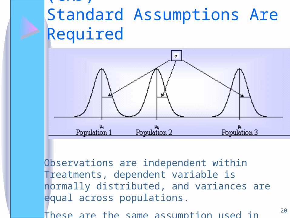
For a One-Way ANOVA (CRD)Standard Assumptions Are Required

Observations are independent within Treatments, dependent variable is normally distributed, and variances are equal across populations.

These are the same assumption used in regression analysis.

21

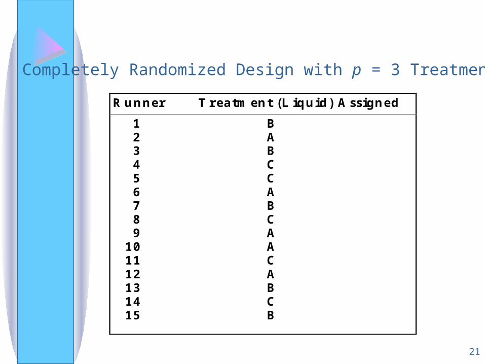
Completely Randomized Design with p = 3 Treatments

R u n n e r T r e a tm e n t (L iq u id ) A s s ig n e d

1 B 2 A 3 B 4 C 5 C 6 A 7 B 8 C 9 A 1 0 A 1 1 C 1 2 A 1 3 B 1 4 C 1 5 B

22

Definition

A randomized block design to compare p treatments involves b blocks, each containing p relatively homogeneous experimental units. The p treatments are randomly assigned to the experimental units within each block, with one experimental unit assigned per treatment.

23

Blocks (Runners) Treatments (Liquids)

1

2

3

4

5

CAB

A C B

B C A

A B C

A C B

24

The model for a completely randomized design would appear as follows:

y = 0 + 1 x1 + 2 x2 +

where

not if 0

Bliquid if 1

not if 0

A liquid if 121

xx

25

From previous discussion of dummy-variable models, we know that the mean responses for the three liquids are

A = 0 + 1

B = 0 + 2

C = 0

26

Similarly, we can write the model for the randomized block design:

effectsBlock

66554433

effects Treatment

22110 xxxxxxy

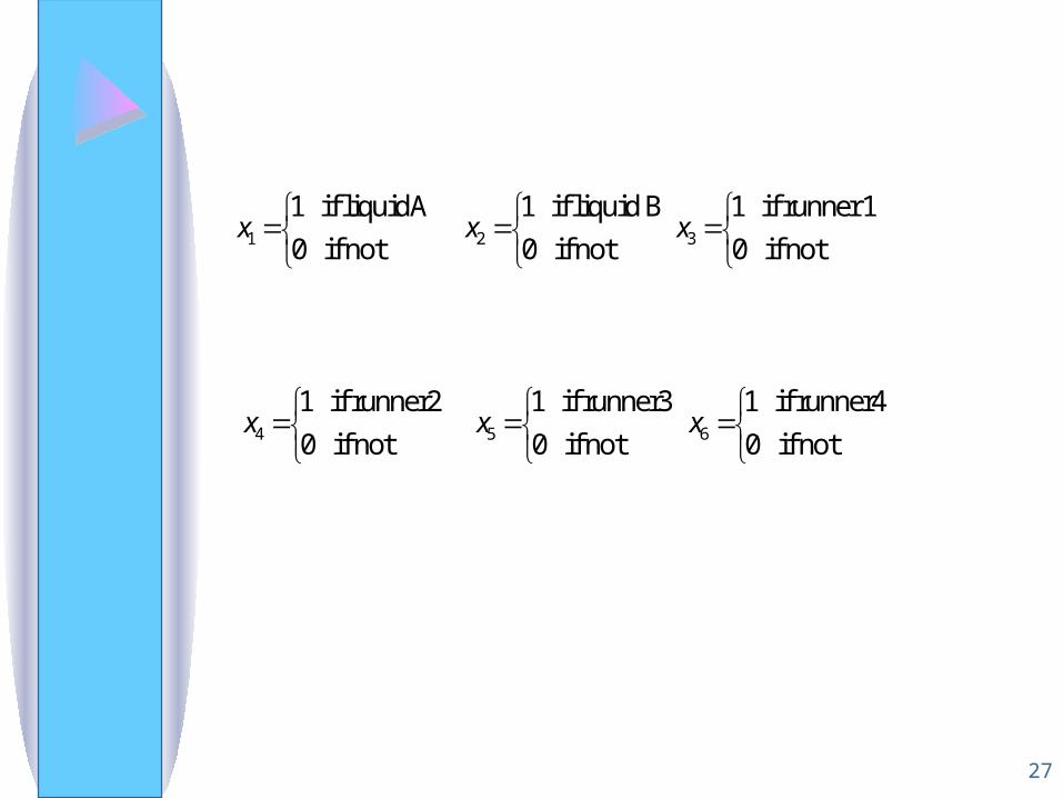
27

not if 0

1runner if 1

not if 0

Bliquid if 1

not if 0

A liquid if 1321

xxx

not if 0

4runner if 1

not if 0

3runner if 1

not if 0

2runner if 1654

xxx

28

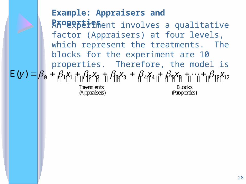
An experiment involves a qualitative factor (Appraisers) at four levels, which represent the treatments. The blocks for the experiment are 10 properties. Therefore, the model is

s)(Propertie

Blocks

12125544

s)(AppraiserTreatments

3322110)E( xxxxxxy

Example: Appraisers and Properties

29

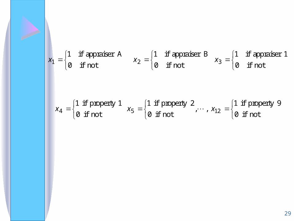
not if 0

1appraiser if 1

not if 0

Bappraiser if 1

not if 0

Aappraiser if 1321

xxx

not if 0

9property if 1 , ,

not if 0

2property if 1

not if 0

1property if 11254

xxx

30

1 = A - D for a given property

2 = B - D for a given property

3 = C - D for a given property

4 = 1 - 10 for a given appraiser

5 = 2 - 10 for a given appraiser

12 = 9 - 10 for a given property

.:

31

One way to determine whether the means for the four appraisers differ is to test the null hypothesis

H0 : A = B = C

H0 : 1 = 2 = 3 = 0

From our interpretations in part b, this hypothesis is equivalent to testing

32

Notation for Experimental Model

• Let be the overall mean. Let i be equal to

i This difference can be thought of as the influence (or effect) of the ith group.

Models for a one-way ANOVA:

Y = 0 + 1 x1 + 2 x2 +

Yij = j + ij

Yij = + j + ij

33

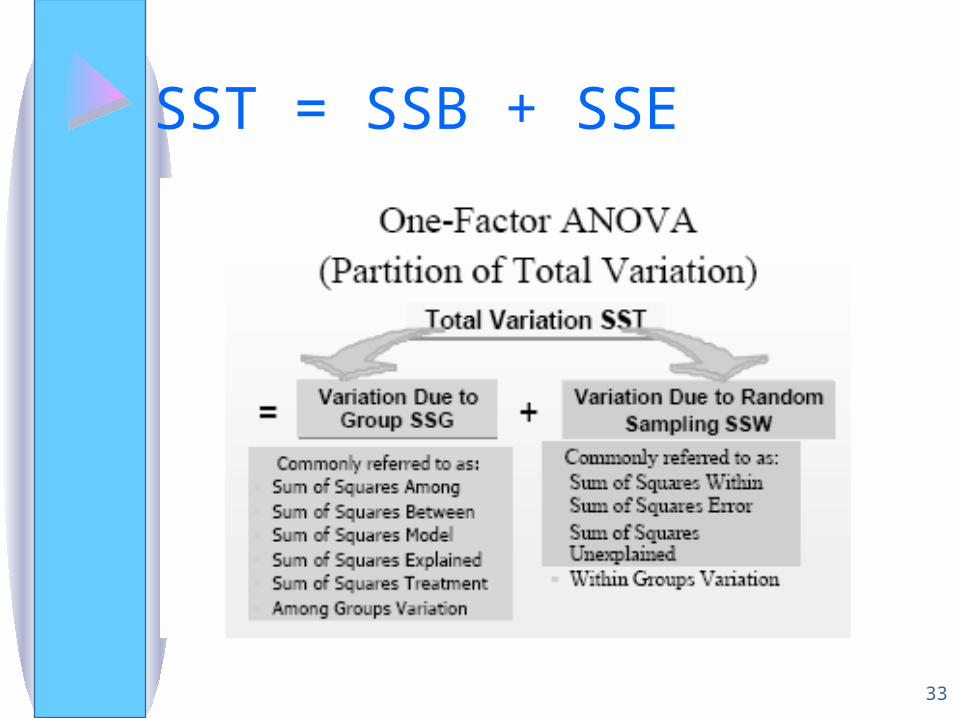
SST = SSB + SSE

34

Objective is to Minimize SSE

ij ij jY2 2 ( )

For a One-way ANOVA, SSE is as follows.

35

Definition : A factorial design is a method for selecting the treatments (that is, the factor level combinations) to be included in an experiment. A complete factorial experiment is one in which the treatments consist of all factor level combinations.

Factorial Design

36

Suppose you plan to conduct an experiment to compare the attitude of adults to internet auctions. In particular, you want to investigate the effect on mean Attitude from three factors:

Income at three levels (A1, A2, and A3) Education at three levels (B!, B2, and B) Age at two levels (C1 and C2). Consider a complete factorial experiment.

Identify the treatments for this 3 x 3 x 2 factorial design.

Factorial Design

37

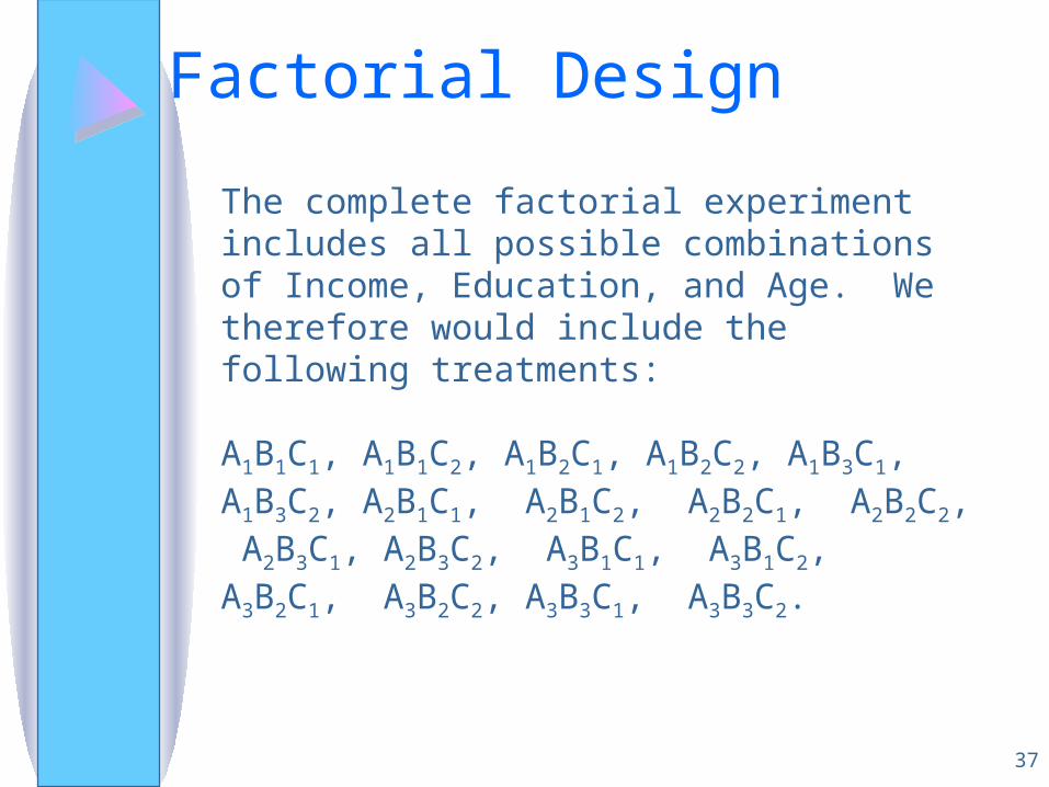
The complete factorial experiment includes all possible combinations of Income, Education, and Age. We therefore would include the following treatments:

A1B1C1, A1B1C2, A1B2C1, A1B2C2, A1B3C1, A1B3C2, A2B1C1, A2B1C2, A2B2C1, A2B2C2, A2B3C1, A2B3C2, A3B1C1, A3B1C2, A3B2C1, A3B2C2, A3B3C1, A3B3C2.

Factorial Design

38

Income Education Age (Treatment)

B1 C1 (1)C2 (2)

A1 B2 C1 (3)C2 (4)

B3 C1 (5)C2 (6)

B1 C1 (7)C2 (8)

A2 B2 C1 (9)C2 (10)

B3 C1 (11)

B1 C2 (12)C1 (13)

A3 B2 C2 (14)C1 (15)

B3 C2 (16)C1 (17)

C2 (18)

39

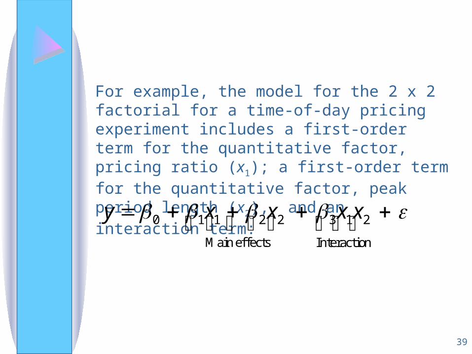
For example, the model for the 2 x 2 factorial for a time-of-day pricing experiment includes a first-order term for the quantitative factor, pricing ratio (x1); a first-order term for the quantitative factor, peak period length (x2), and an interaction term:

nInteractio

213

effectsMain

22110 xxxxy

40

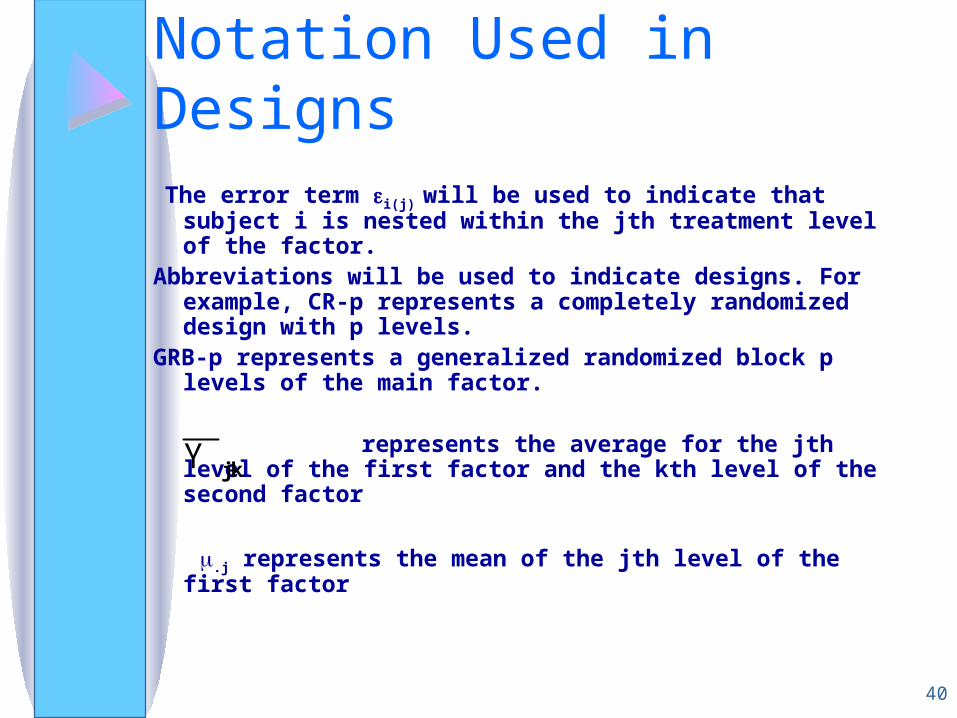
Notation Used in DesignsThe error term i(j) will be used to indicate that subject i is

nested within the jth treatment level of the factor. Abbreviations will be used to indicate designs. For example,

CR-p represents a completely randomized design with p levels.

GRB-p represents a generalized randomized block p levels of the main factor.

represents the average for the jth level of the first

factor and the kth level of the second factor

.j represents the mean of the jth level of the first factor

Y . jk

41

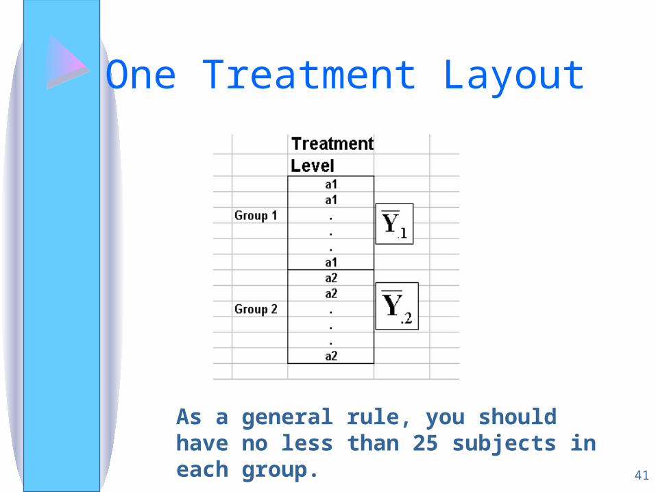
One Treatment Layout

As a general rule, you should have no less than 25 subjects in each group.

42

One Group Should be Selected as the Control or Baseline Group

• Matched subjects, or subjects, in the control group are NOT to be exposed to some treatment, intervention, or change that you introduce or manipulate. You can have more than one control and treatment group.

43

Fixed-Effects Model and Random Effects Model

• Fixed-effects models: All treatment levels about which inferences are drawn are included in the experiment.

• Random-effects model: Treatment levels included in the experiment are a random sample from a much larger population. For example, random time intervals may be selected.

44

Review Rules of Summation andRules of Expectation, Variance, andCovariance

Appendix A:

Many Sums will look complicated, but all them can be found by using Rules A.1 through A.6.

Appendix B:

Expected values of Mean Sums of Squares will be presented. These Expected values are found using these rules.

45

Adding a Constant to Design Model

• The values of sums of squares will not change when a constant is added. The individual parts of the calculation may change, the final sum will not.

• Sums of Squares represent variances. Look at Rule B.14: V(c + Y) = V(Y).

46

Homework 1 (TBA)