1 preferred citation style matsim development team (ed.) (2007) matsim-t: aims, approach and...
TRANSCRIPT
1
Preferred citation style
MATSim development team (ed.) (2007) MATSIM-T: Aims, approach and implementation, IVT, ETH Zürich, Zürich.
MATSIM-T: Aims, approach and implementation
August 2007
3
Overview
• Structure and team• Task and solution methods• MATSIM aims
• System architecture• Examples
• Switzerland• Berlin/Brandenburg
• Outlook and next steps
• Progress on shortest path calculations• Traffic flow model• Improving the convergence
4
Structure
Software:
• Open-source project under GNU public licence
Coordination:
• Kai Nagel, TU Berlin
Data:
• Public sources, where available• Private sources, when needed or as occasion arises
5
Current team
Strategy:
• Kai Nagel, TU Berlin
• Kay Axhausen, ETH Zürich• Fabrice Marchal, LET, Lyon
Coordination of the implementation and project management:
• Michael Balmer, ETH Zürich
• Marcel Rieser, TU Berlin
6
Current team: Implementation (1/2)
• Michael Balmer, ETH• David Charypar, ETH• Francesco Ciari, ETH• Dominik Grether, TU Berlin• Jeremy Hackney, ETH• Andreas Horni, ETH• Gregor Lämmel, TU Berlin• Nicolas Lefebvre, ETH• Michael Löchl, ETH
7
Current team: Implementation (2/2)
• Fabrice Marchal, LET• Konrad Meister, ETH• Kai Nagel, TU Berlin• Marcel Rieser, TU Berlin• Nadine Schüssler, ETH• David Strippgen, TU Berlin

8
Current funding sources
• Basic research support for the chairs
• (competitive) ETH research fund• Swiss National Fund• German Research Society• EU Framework funding• VW Foundation• Swiss Commission for Technology and Information (KTI)
(datapuls, Lucerne)
9
Task and solution methods
10
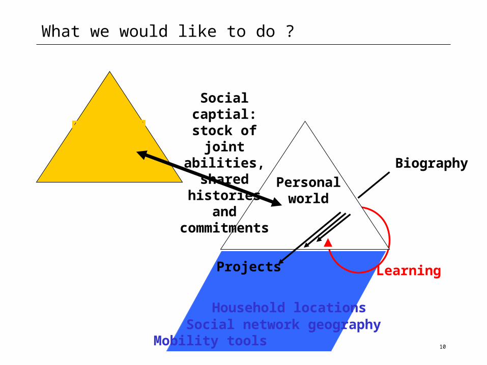
What we would like to do ?
Personalworld
Biography
Projects Learning
Personalworlds of
others
Social captial: stock of
joint abilities, shared
histories and
commitments
Household locations Social network geographyMobility tools
11
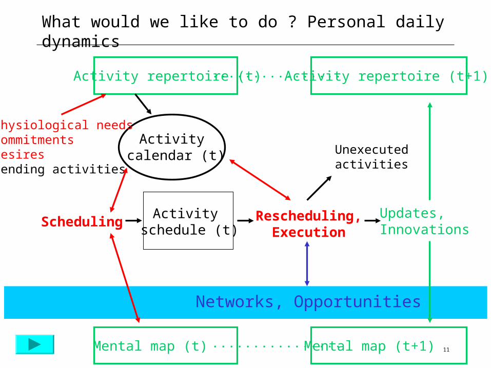
What would we like to do ? Personal daily dynamics
Activity repertoire (t) Activity repertoire (t+1) ................
Activity calendar (t)
Physiological needsCommitmentsDesiresPending activities
Activity schedule (t)
Mental map (t) Mental map (t+1) ................
Scheduling
Networks, Opportunities
Rescheduling,Execution
Updates,Innovations
Unexecutedactivities
12
Understanding scheduling
• Budget constraints • Capability constraints
• Generalised costs of the schedule
• Generalised cost of travel• Generalised cost of activity participation
• Risk and comfort-adjusted weighted sums of time, expenditure and social content
13
Degrees of freedom of activity scheduling
• Number and type of activities• Sequence of activities
• Start and duration of activity• Composition of the group undertaking the activity• Location of the activity
• Connection between sequential locations
• Location of access and egress from the mean of transport
• Vehicle/means of transport• Route/service• Group travelling together
14
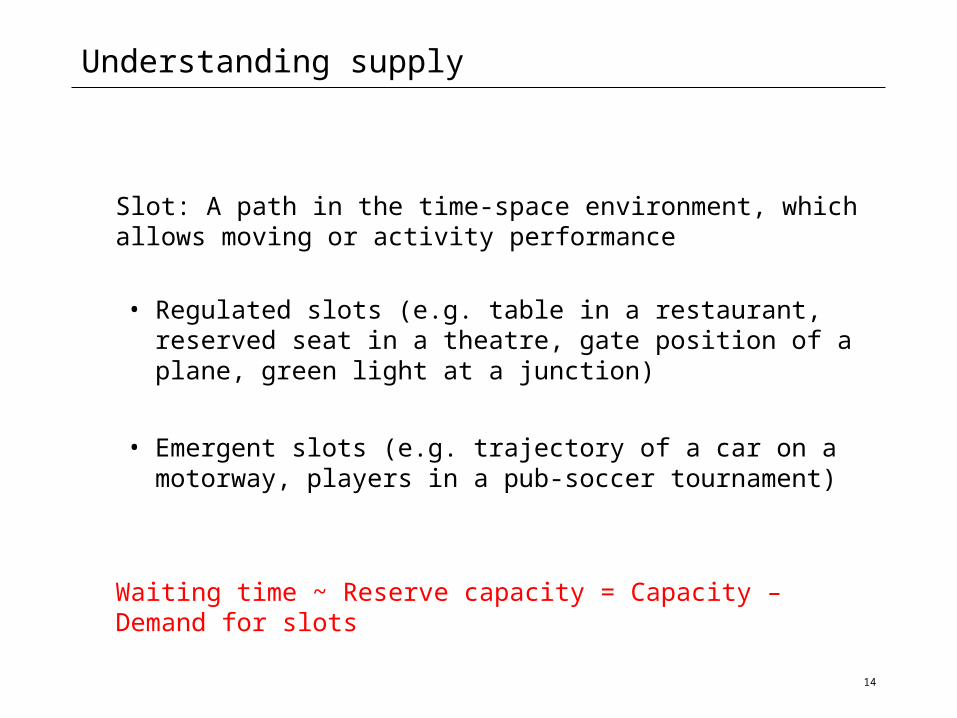
Understanding supply
Slot: A path in the time-space environment, which allows moving or activity performance
• Regulated slots (e.g. table in a restaurant, reserved seat in a theatre, gate position of a plane, green light at a junction)
• Emergent slots (e.g. trajectory of a car on a motorway, players in a pub-soccer tournament)
Waiting time ~ Reserve capacity = Capacity – Demand for slots
15
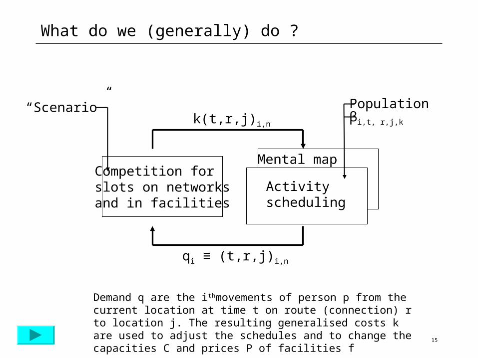
What do we (generally) do ?
Competition for slots on networks and in facilities
k(t,r,j)i,n
qi ≡ (t,r,j)i,n
βi,t, r,j,k
Population “Scenario”
Activity scheduling
Mental map
Demand q are the ithmovements of person p from the current location at time t on route (connection) r to location j. The resulting generalised costs k are used to adjust the schedules and to change the capacities C and prices P of facilities f
16
Classification criteria
• Steady state (equilibrium) ?
• Aggregate demands ?
• Complete and perfect knowledge ?
• Optimised schedules ?
• Degrees of freedom and detail of scheduling
• Modelling of capacity restrictions (movement, activities) ?
17
MATSIM-T aims (1): Steady-state version
• Steady state within 12 hours on a small multi-CPU machine
• 7.5 mio agents, parcels, navigation networks
• Shared time-of-day dependent generalised costs of travel and activity participation
• Optimised schedules• Continuous time resolution; space: parcels; social networks
• Queuing for slots for movement and activities
18
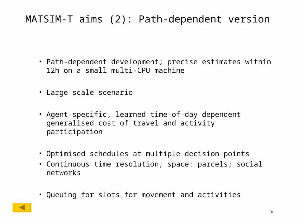
MATSIM-T aims (2): Path-dependent version
• Path-dependent development; precise estimates within 12h on a small multi-CPU machine
• Large scale scenario
• Agent-specific, learned time-of-day dependent generalised cost of travel and activity participation
• Optimised schedules at multiple decision points• Continuous time resolution; space: parcels; social networks
• Queuing for slots for movement and activities
19
System architecture
• XML standards
• Data handling tools (aggregation/disaggregation)
• Data base
• Iteration handling and control of convergence
• Models
20
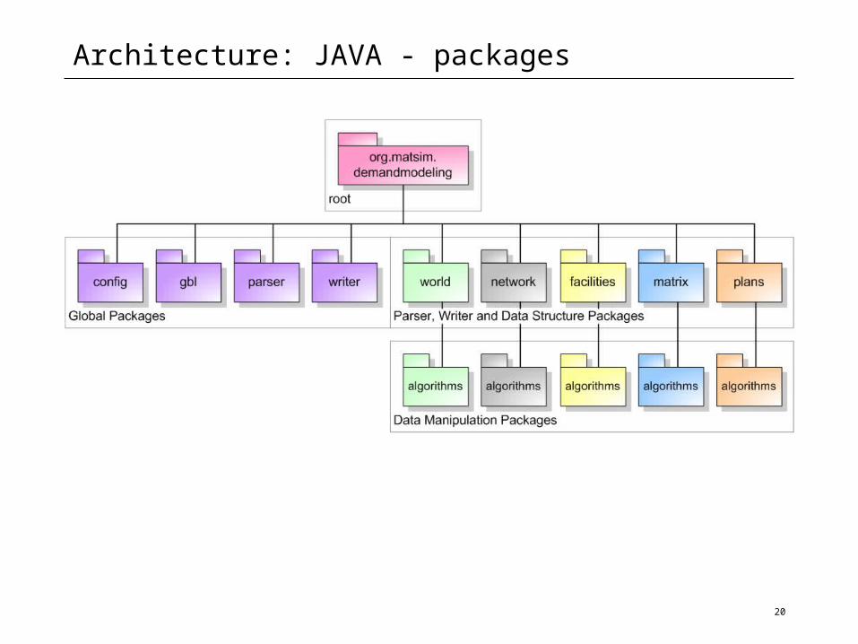
Architecture: JAVA - packages
21
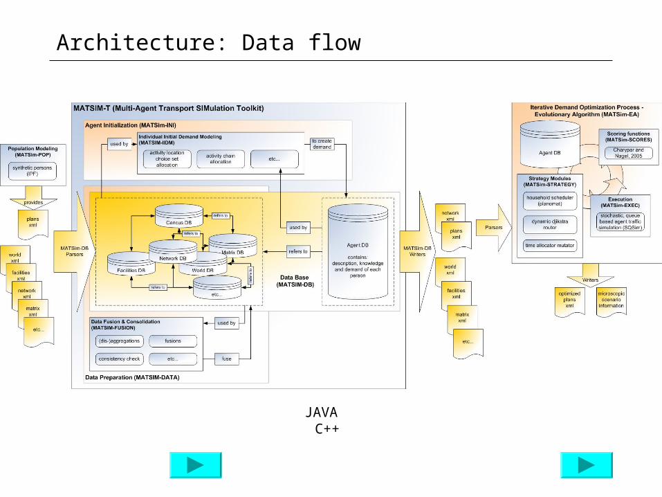
Architecture: Data flow
JAVA C++
22
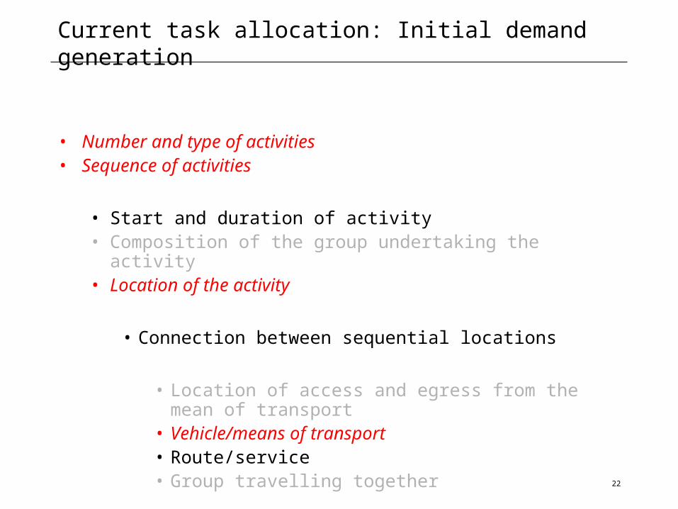
Current task allocation: Initial demand generation
• Number and type of activities• Sequence of activities
• Start and duration of activity• Composition of the group undertaking the activity• Location of the activity
• Connection between sequential locations
• Location of access and egress from the mean of transport
• Vehicle/means of transport• Route/service• Group travelling together
23
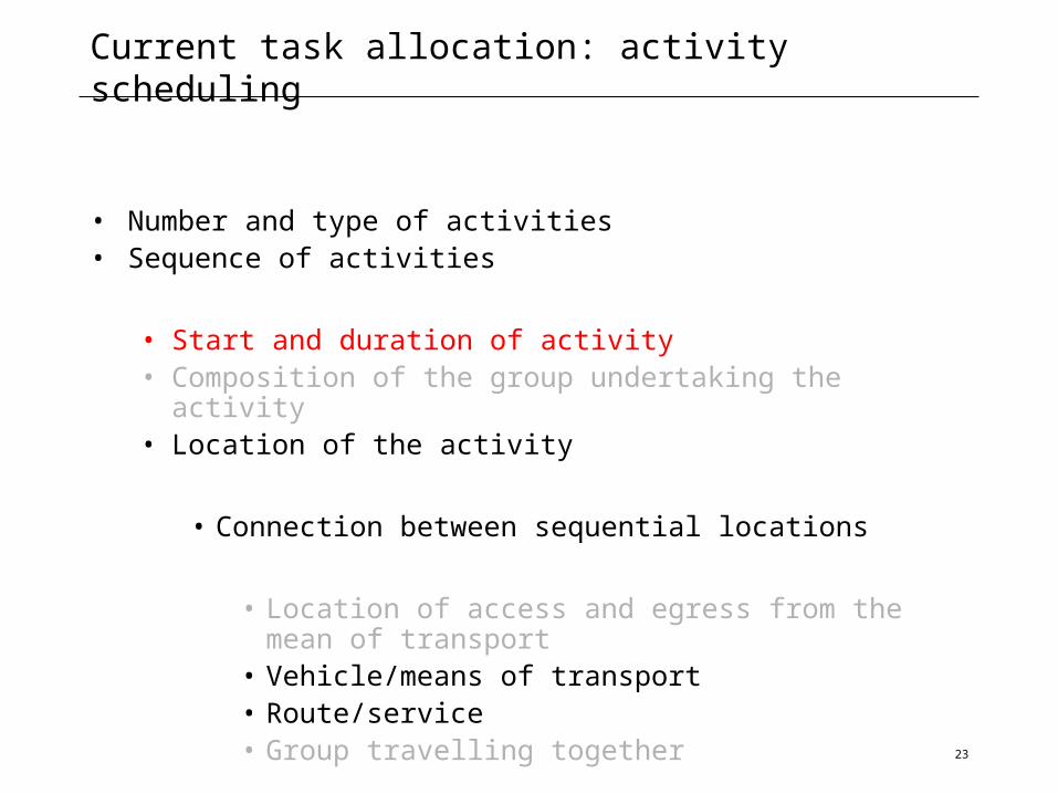
Current task allocation: activity scheduling
• Number and type of activities• Sequence of activities
• Start and duration of activity• Composition of the group undertaking the activity• Location of the activity
• Connection between sequential locations
• Location of access and egress from the mean of transport
• Vehicle/means of transport• Route/service• Group travelling together
24
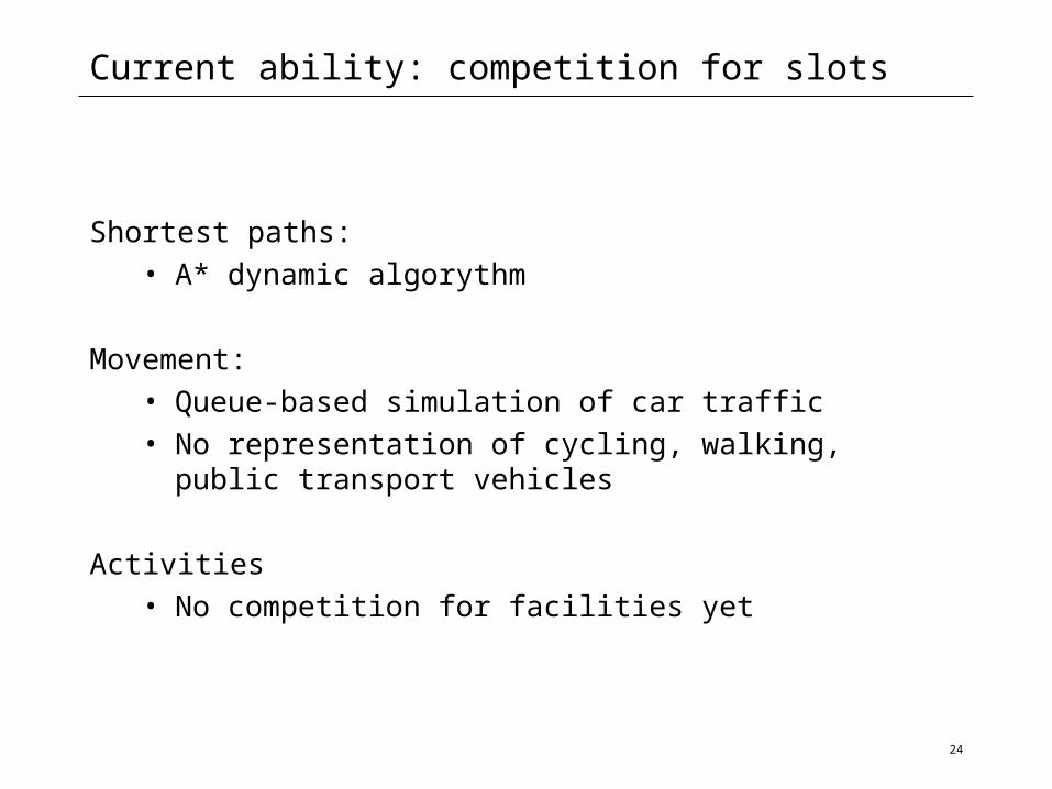
Current ability: competition for slots
Shortest paths:• A* dynamic algorythm
Movement: • Queue-based simulation of car traffic• No representation of cycling, walking, public transport
vehicles
Activities• No competition for facilities yet
25
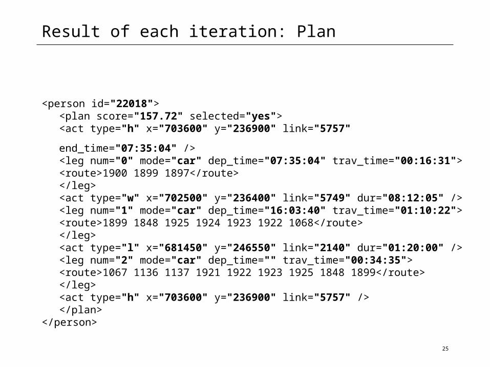
Result of each iteration: Plan
<person id="22018"><plan score="157.72" selected="yes">
<act type="h" x="703600" y="236900" link="5757" end_time="07:35:04" /><leg num="0" mode="car" dep_time="07:35:04" trav_time="00:16:31">
<route>1900 1899 1897</route></leg><act type="w" x="702500" y="236400" link="5749" dur="08:12:05" /><leg num="1" mode="car" dep_time="16:03:40" trav_time="01:10:22">
<route>1899 1848 1925 1924 1923 1922 1068</route></leg><act type="l" x="681450" y="246550" link="2140" dur="01:20:00" /><leg num="2" mode="car" dep_time="" trav_time="00:34:35">
<route>1067 1136 1137 1921 1922 1923 1925 1848 1899</route>
</leg><act type="h" x="703600" y="236900" link="5757" />
</plan></person>
26
Scheduling and its utility function
27
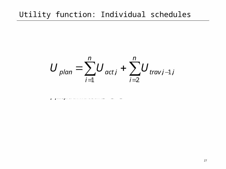
Utility function: Individual schedules
∑∑=
−=
+=n
iiitrav
n
iiactplan UUU
2,1,
1,
,,.,actidurilateariUUU=+
28
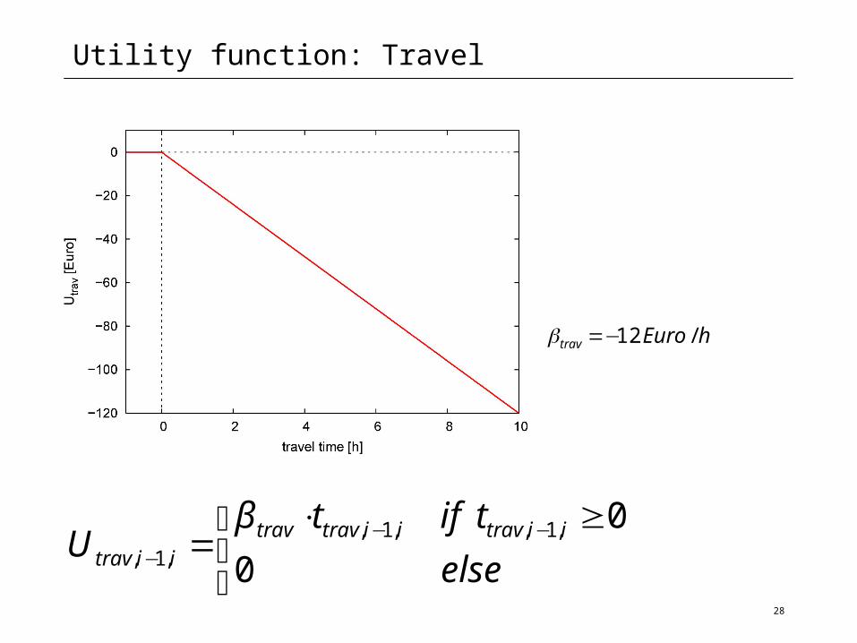
Utility function: Travel
⎩⎨⎧ ≥⋅
= −−− else
tiftU iitraviitravtrav
iitrav 0
0,1,,1,,1,
β
hEurotrav /12−=β
29
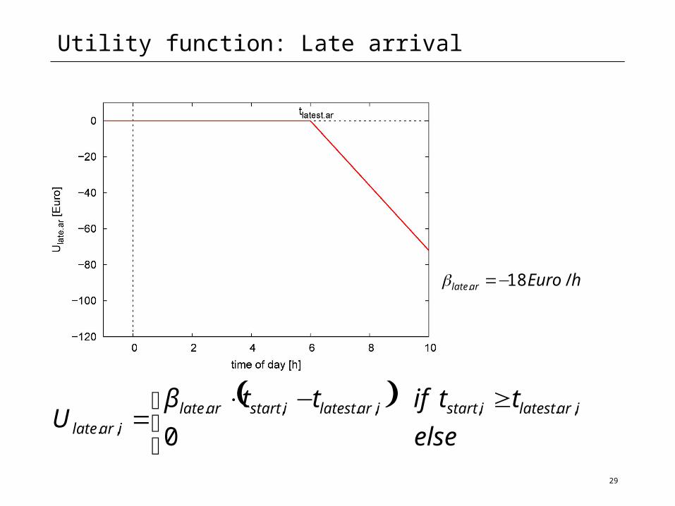
Utility function: Late arrival
( )⎩⎨⎧ ≥−⋅
=else
ttifttU iarlatestistartiarlatestistartarlate
iarlate 0,.,,.,.
,.
β
hEuroarlate /18. −=β
30
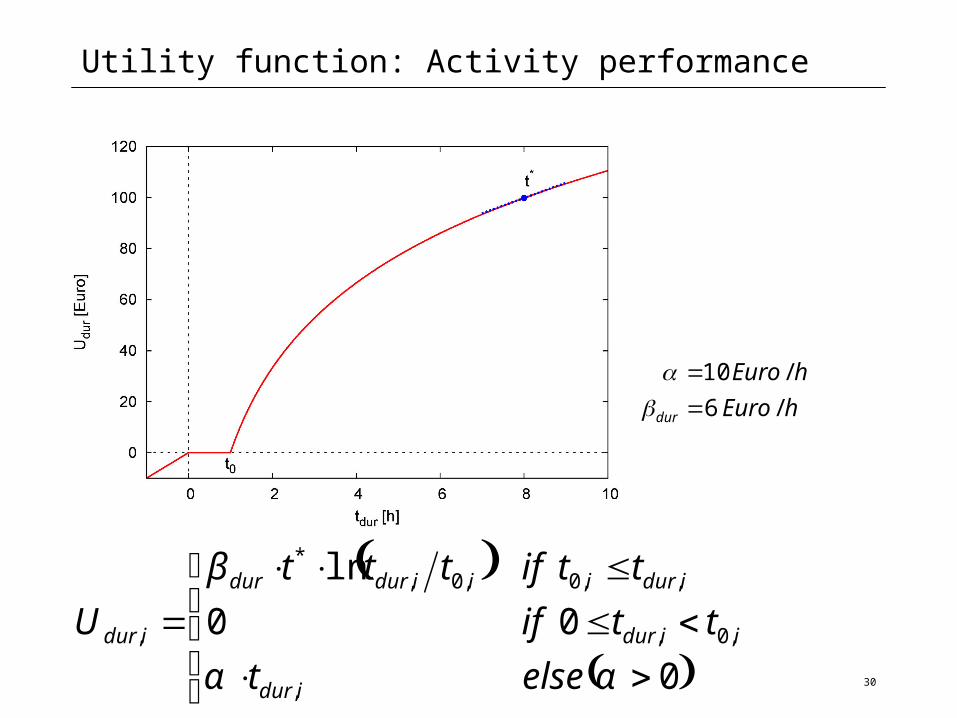
Utility function: Activity performance
( )
( )⎪⎩
⎪⎨
⎧
>⋅<≤
≤⋅⋅=
0
00
ln
,
,0,
,,0,0,*
,
αα
β
elset
ttif
ttifttt
U
idur
iidur
iduriiidurdur
idur
hEuro
hEuro
dur /6
/10
==
βα
31
Scheduling: Current planomat(s)
Version 1:
• GA optimiser of durations and starting times• Retains time-of-day profile of generalised costs
Version 2:
• CMA-ES (Covariance Matrix Adaptation Evolutionary strategy) of durations and starting times
• Retains time-of-day profile of generalised costs
32
Examples (scenarios):
• CH: Switzerland and subsets• Base tests for Kanton Zürich
• B/B: Berlin/Brandenburg• Tolling case studies
33
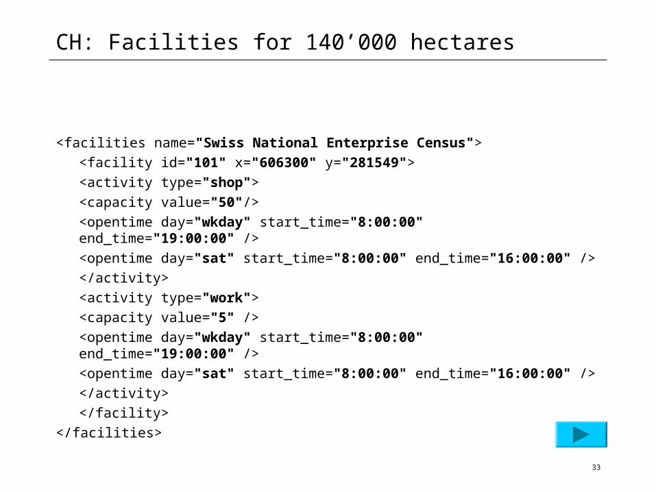
CH: Facilities for 140’000 hectares
<facilities name="Swiss National Enterprise Census">
<facility id="101" x="606300" y="281549">
<activity type="shop">
<capacity value="50"/>
<opentime day="wkday" start_time="8:00:00" end_time="19:00:00" />
<opentime day="sat" start_time="8:00:00" end_time="16:00:00" />
</activity>
<activity type="work">
<capacity value="5" />
<opentime day="wkday" start_time="8:00:00" end_time="19:00:00" />
<opentime day="sat" start_time="8:00:00" end_time="16:00:00" />
</activity>
</facility>
</facilities>
34
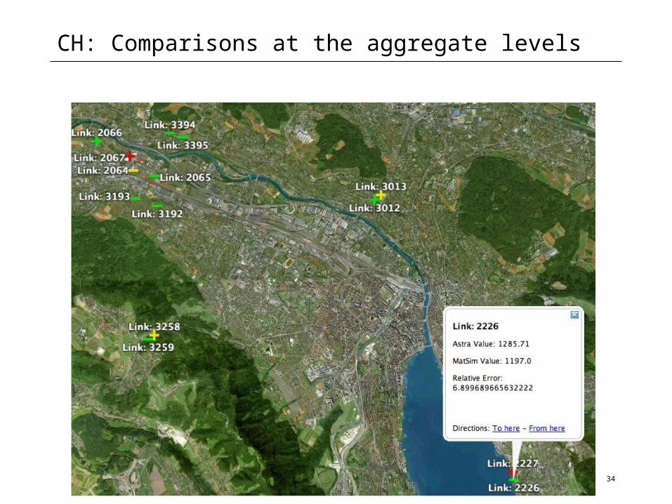
CH: Comparisons at the aggregate levels
35
CH: Network
Simplification:
• Remove unconnected links and subnetworks• Remove nodes between unchanging link types• Cut off dead ends
Results:
• Navteq (882’120 links) (25% loss of links/nodes)
• Teleatlas (1’288’757 links) (currently not in use)
36
CH: Population
Alternatives:
• Artificial sample generation from Census marginals
• Census
• Private census with additional imputations (datapuls, Lucerne) plus household “formation”
37
CH: Mobility tools
Approach:
• MNL of mobility tool packages (Beige)
• Socio-demographics• Location types• Travel times to main centre by road and public transport
Data:
• National travel survey (MZ 2000)
38
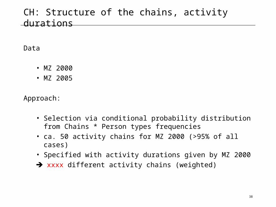
CH: Structure of the chains, activity durations
Data
• MZ 2000• MZ 2005
Approach:
• Selection via conditional probability distribution from Chains * Person types frequencies
• ca. 50 activity chains for MZ 2000 (>95% of all cases)• Specified with activity durations given by MZ 2000
xxxx different activity chains (weighted)
39
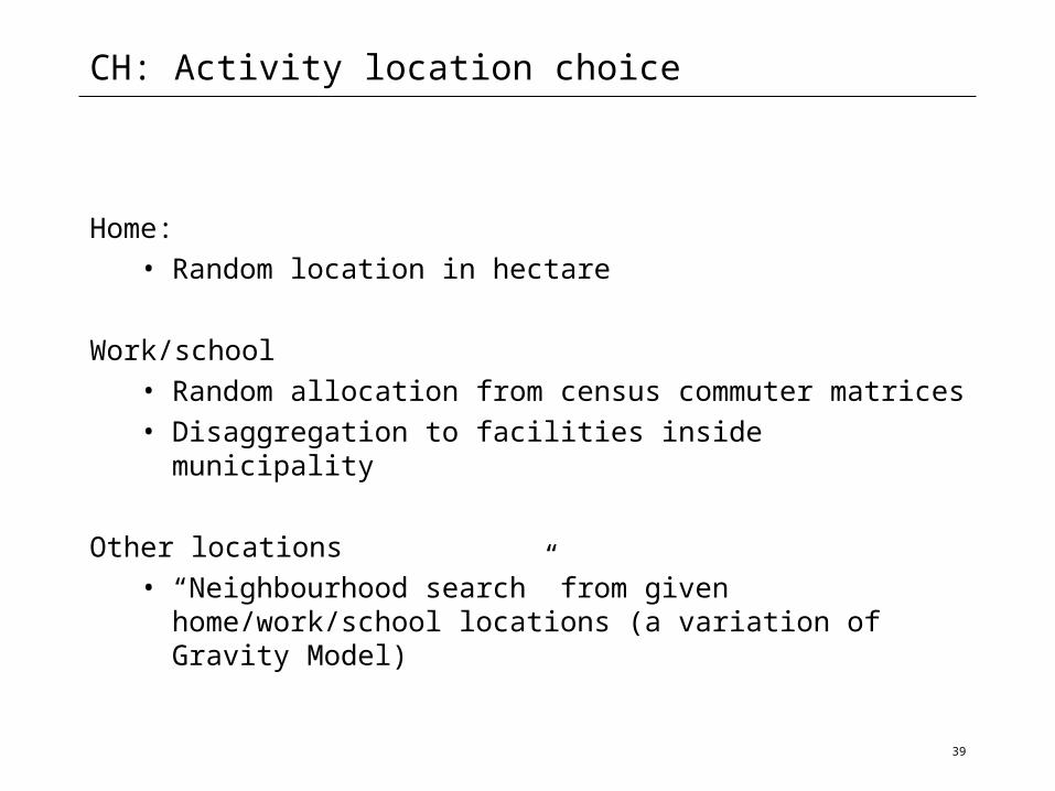
CH: Activity location choice
Home:• Random location in hectare
Work/school• Random allocation from census commuter matrices• Disaggregation to facilities inside municipality
Other locations• “Neighbourhood search” from given home/work/school
locations (a variation of Gravity Model)
40
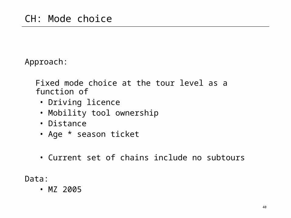
CH: Mode choice
Approach:
Fixed mode choice at the tour level as a function of• Driving licence• Mobility tool ownership• Distance• Age * season ticket
• Current set of chains include no subtours
Data:• MZ 2005
41
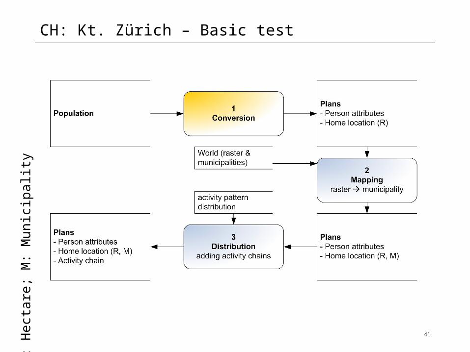
CH: Kt. Zürich – Basic testR
: He
cta
re; M
: Mu
nic
ipa
lity
42
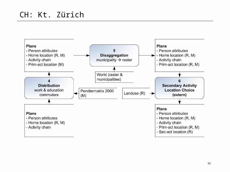
CH: Kt. Zürich
43
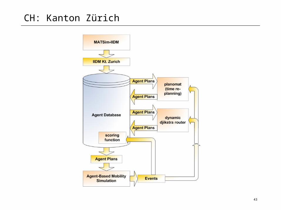
CH: Kanton Zürich
44
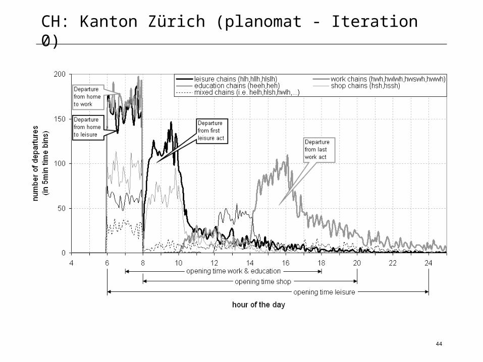
CH: Kanton Zürich (planomat - Iteration 0)
45
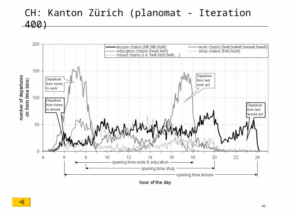
CH: Kanton Zürich (planomat - Iteration 400)
46
B/B: Network
• Source: “Senatsverwaltung für Stadtentwicklung Berlin”
• 11596 nodes • 27770 links
47
B/B: Population and demand
• Generated from “Kutter-Nachfragemodell für Berlin”,
• only commuters (work, education) in Berlin/Brandenburg,
• only car-trips simulated,
• 10% sample: 160’171 agents, each with 2 trips
• Facilities = traffic analysis zones
48
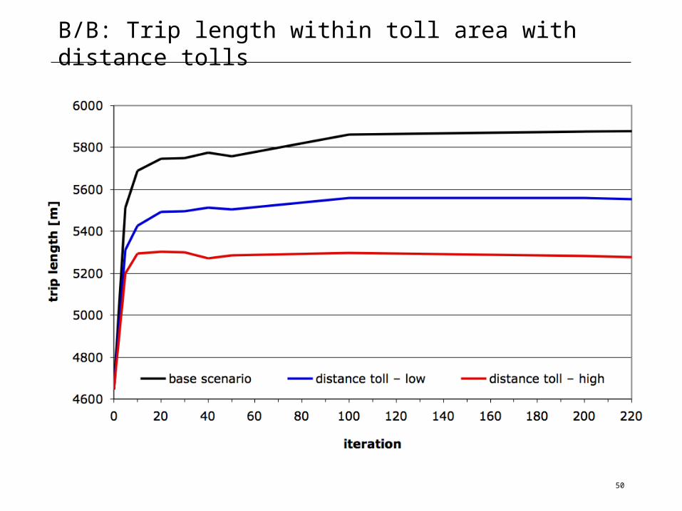
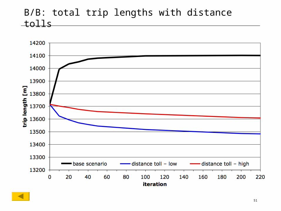
B/B: Tolling in Berlin/Brandenburg
• Scenario: As described above
• Aims: Impacts of distance and area tolls
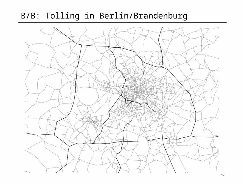
49
B/B: Tolling in Berlin/Brandenburg
50
B/B: Trip length within toll area with distance tolls
51
B/B: total trip lengths with distance tolls

52
Outlook
53
Current tasks: Functionality
• Improving the realism of the scenario (e.g. opening hours, parameter distributions)
• Validation of the current scenarios• Switzerland scenario in 12h to steady state
• Functional expansion the planomat (mode choice, destination choice)
• Parameter estimation for planomat
• Interface to UrbanSim
54
Future tasks: Functionality
• Integration of social network data structures • Explicit social network choices
• Addition of supply agents (car sharing, demand responsive transport, retail location, parking pricing, road pricing) (Traffic control)
55
Current tasks: Usability (Shareability)
• Analysis tools
• Anonymous test data sets
• Improved documentation
• Web and sourceforge maintenance
• User support, including visits to ETH/TU Berlin

56
Acknowledgements (1/3)
System architecture: Michael BalmerSystem integration: Michael Balmer, Marcel RieserSystem management: Michael Balmer, Marcel Rieser
Facilities: Konrad MeisterMobility tools: Francesco CiariTour mode choice: Francesco Ciari
Counter infrastructure: Andreas Horni
KML – interfaces: Konrad Meister, Dominik Grether
57
Acknowledgements (2/3)
Router: Nicolas Lefebvre
Traffic flow model: David Charypar
Planomat: Konrad Meister, David Charypar
Supply agents: Michael Löchl, Francesco Ciari
Social networks: Jeremy Hackney
58
Acknowledgements (3/3)
Past contributors:
• Michael Bernard, ETH • Sigrun Beige, ETH• Ulrike Beuck, TU-Berlin• Dr. Nurhan Cetin (ETH)• Phillip Fröhlich, Modus, Zürich (ETH)• Dr. Christian Gloor (ETH)• Dr. Bryan Raney, HP America (ETH)• Marc Schmitt (ETH)• Arnd Vogel, PTV (TU Berlin)
59
More information
www.matsim.org
www.vsp.tu-berlin.de
www.ivt.ethz.ch/vpl/publications/reports
60
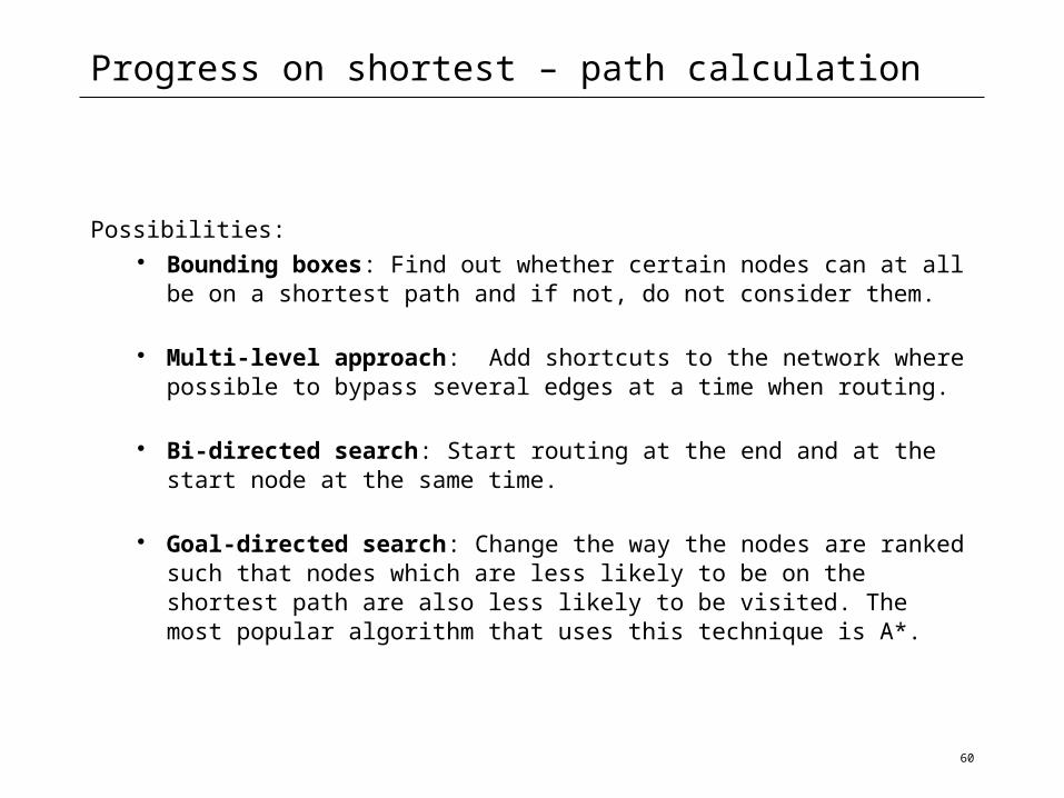
Progress on shortest – path calculation
Possibilities: Bounding boxes: Find out whether certain nodes can at all be on
a shortest path and if not, do not consider them.
Multi-level approach: Add shortcuts to the network where possible to bypass several edges at a time when routing.
Bi-directed search: Start routing at the end and at the start node at the same time.
Goal-directed search: Change the way the nodes are ranked such that nodes which are less likely to be on the shortest path are also less likely to be visited. The most popular algorithm that uses this technique is A*.
61
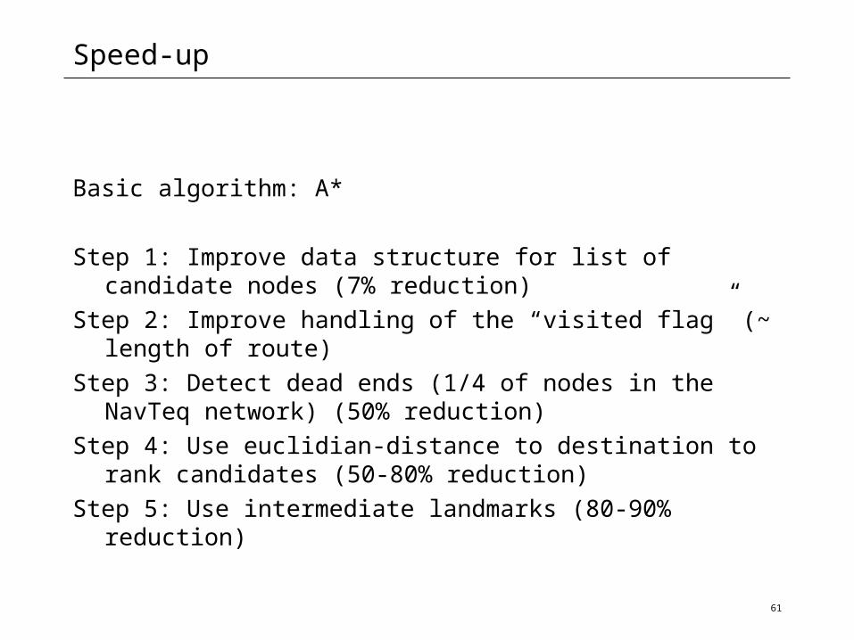
Speed-up
Basic algorithm: A*
Step 1: Improve data structure for list of candidate nodes (7% reduction)
Step 2: Improve handling of the “visited flag” (~ length of route)
Step 3: Detect dead ends (1/4 of nodes in the NavTeq network) (50% reduction)
Step 4: Use euclidian-distance to destination to rank candidates (50-80% reduction)
Step 5: Use intermediate landmarks (80-90% reduction)

62
Landmark selection
• Divide network into sectorscontaining an equal numberof nodes
• For each sector, choosea node that is farthestaway from the center
• Check that thelandmarks are nottoo close to eachother. If so, narrowone sector and choosea new landmark within the sector
63
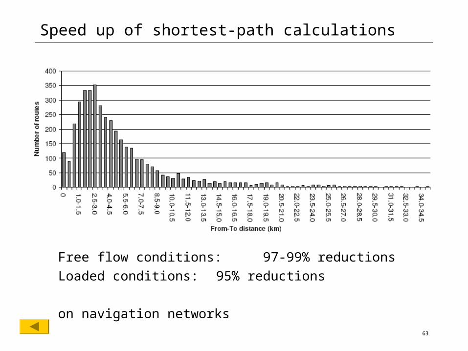
Speed up of shortest-path calculations
Free flow conditions: 97-99% reductions
Loaded conditions: 95% reductions
on navigation networks
64
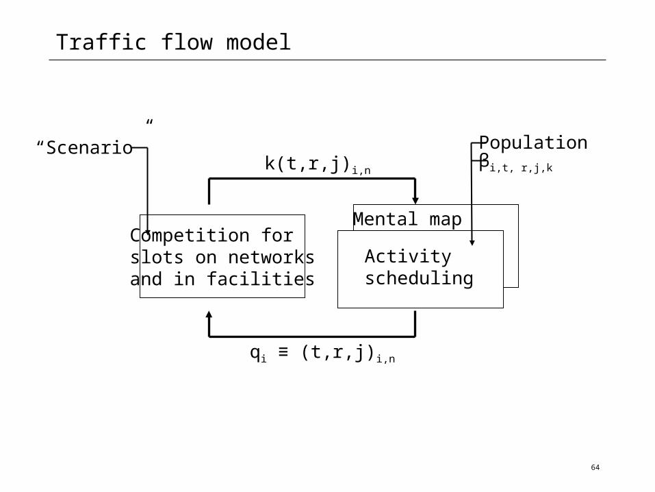
Traffic flow model
Competition for slots on networks and in facilities
k(t,r,j)i,n
qi ≡ (t,r,j)i,n
βi,t, r,j,k
Population “Scenario”
Activity scheduling
Mental map
65
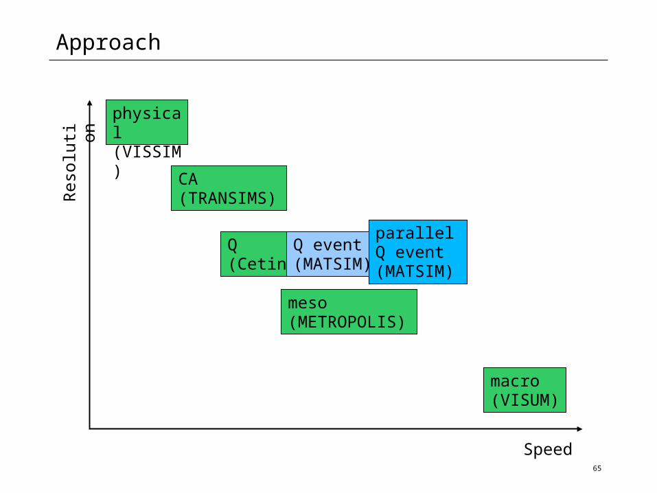
Approach
Speed
Res
olut
ion
physical(VISSIM)
CA(TRANSIMS)
meso(METROPOLIS)
macro(VISUM)
Q(Cetin)
Q event(MATSIM)
parallelQ event(MATSIM)
66
Parallel q-event driven simulation with gaps
• Approach
• Fundamental diagram (on a ring motorway)
• Domain decomposition
• Test
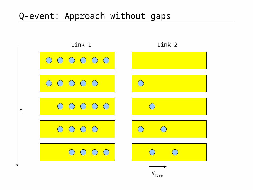
Q-event: Approach without gaps
t
Link 1 Link 2
vfree
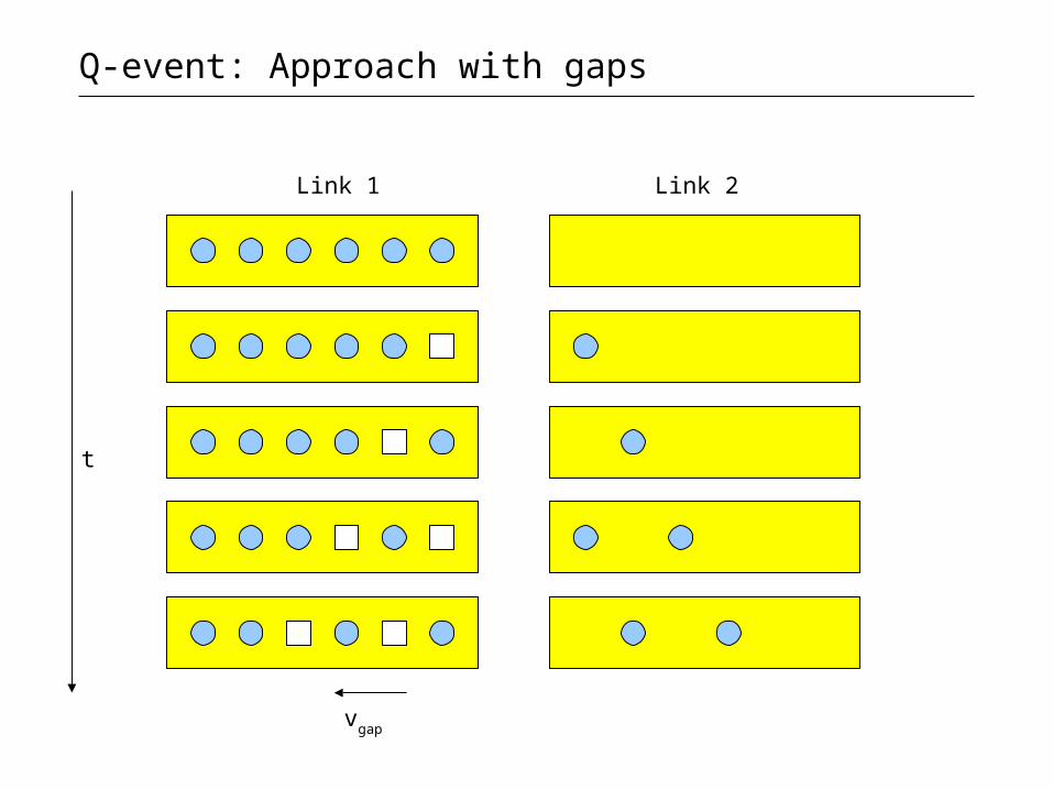
Q-event: Approach with gaps
t
Link 1 Link 2
vgap
69
Q-event: Implementation details
• Squeezing to avoid grid-lock
• Inflow capacity = 110% of outflow capacity (1800 veh/h* lanes)
• Vehicles are served in order of arrival at the junctions
• C++ with binary data interface to MATSim-T
70
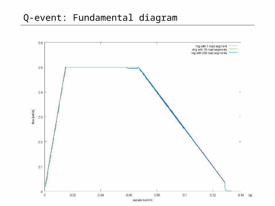
Q-event: Fundamental diagram
Q-event: Test setup
• Road network of the federal states of Germany Berlin and Brandenburg
• 11.6k nodes, 27.7k links
• 7.05M person days• Average number of trips per agent: 2.02• Average length of a trip: 17.5 links• Total: 249M road segments to be traveled
• 77 min on a single dual-core CPU (1.6GH; 256 GB RAM)
72
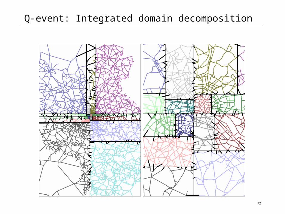
Q-event: Integrated domain decomposition
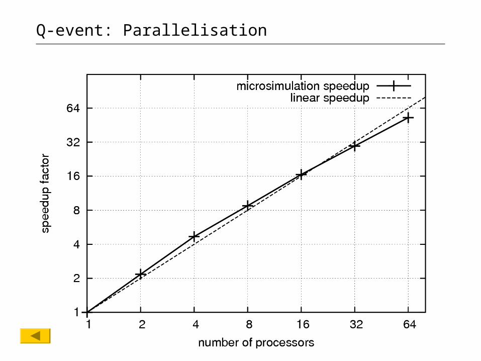
Q-event: Parallelisation

74
Improving the convergence
75
Initial approach
Method:
• Plan everybody at Iteration 1• Replan for a fixed share
Convergence:
• On mean performance
76
Improved approach
Method:
• Plan for everyone at Iteration 1• Replan for a predetermined, but decreasing share over the
number of iterations
Measurement:
• Aggregates
77
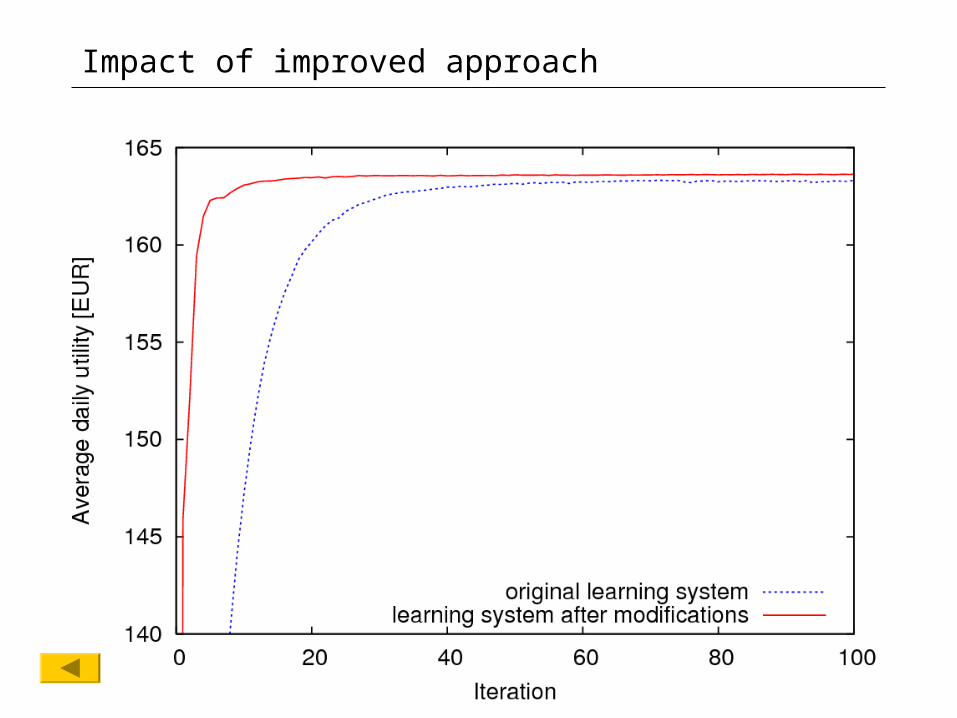
Impact of improved approach

78
Support graphs and further ideas
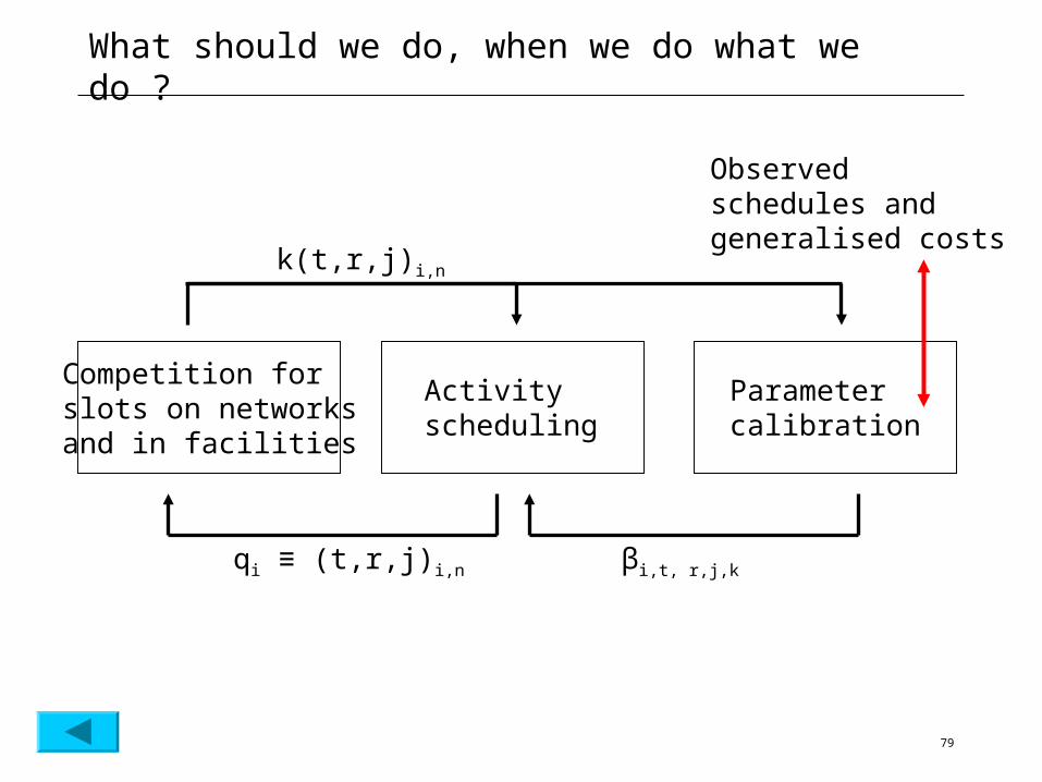
79
What should we do, when we do what we do ?
Competition for slots on networks and in facilities
Activity scheduling
k(t,r,j)i,n
qi ≡ (t,r,j)i,n
Parameter calibration
βi,t, r,j,k
Observed schedules andgeneralised costs
80
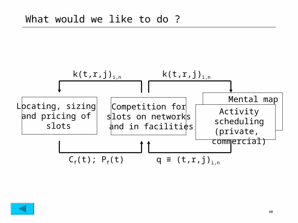
What would we like to do ?
Competition for slots on networks
and in facilities
Activity scheduling(private,
commercial)
k(t,r,j)i,n
q ≡ (t,r,j)i,n
Mental mapLocating, sizing and pricing of
slots
Cf(t); Pf(t)
k(t,r,j)i,n
81
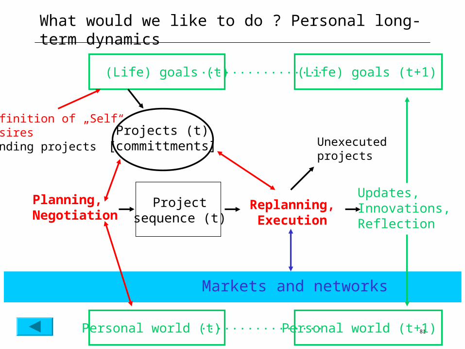
What would we like to do ? Personal long-term dynamics
(Life) goals (t) (Life) goals (t+1) ................
Projects (t)[committments]
Definition of „Self“DesiresPending projects
Projectsequence (t)
Personal world (t) Personal world (t+1) ................
Planning, Negotiation
Markets and networks
Replanning,Execution
Updates,Innovations,Reflection
Unexecutedprojects
82
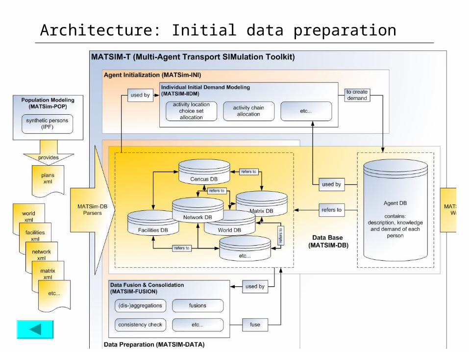
Architecture: Initial data preparation
83
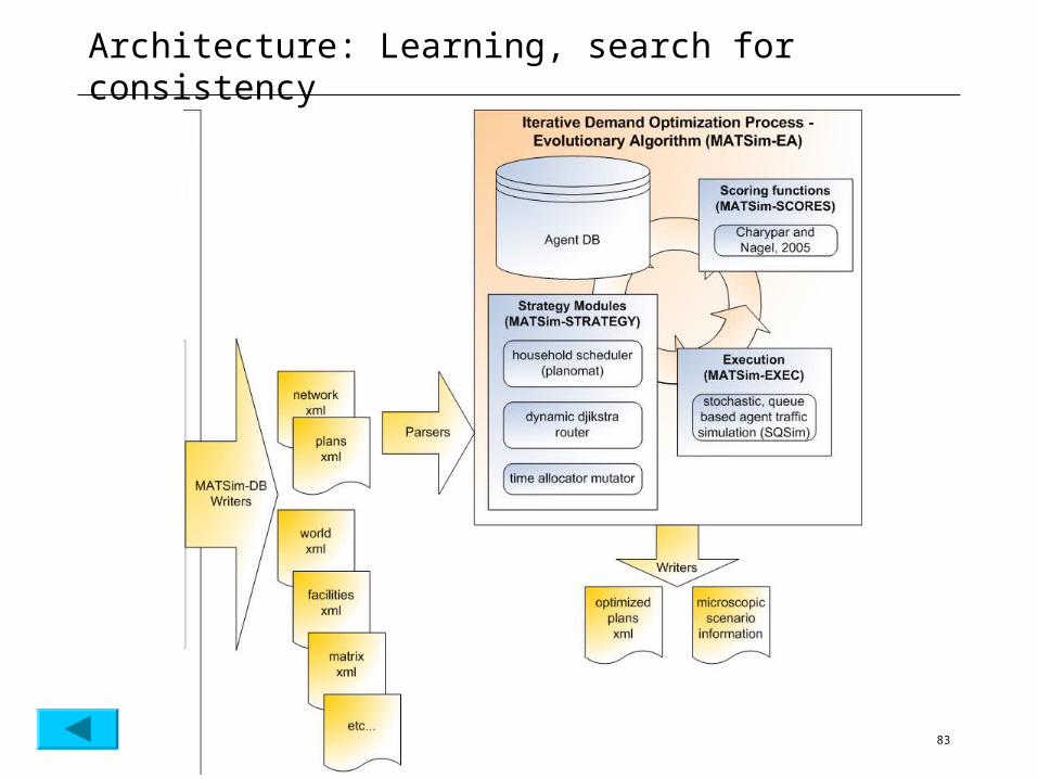
Architecture: Learning, search for consistency
84
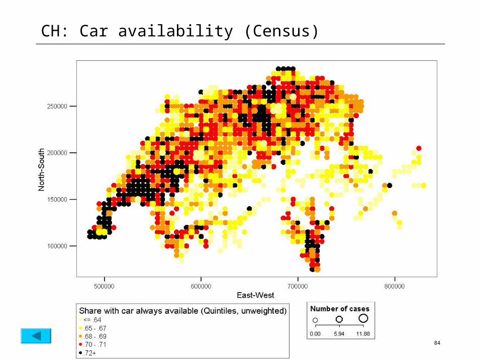
CH: Car availability (Census)
85
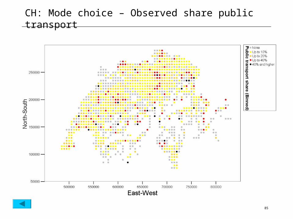
CH: Mode choice – Observed share public transport
86
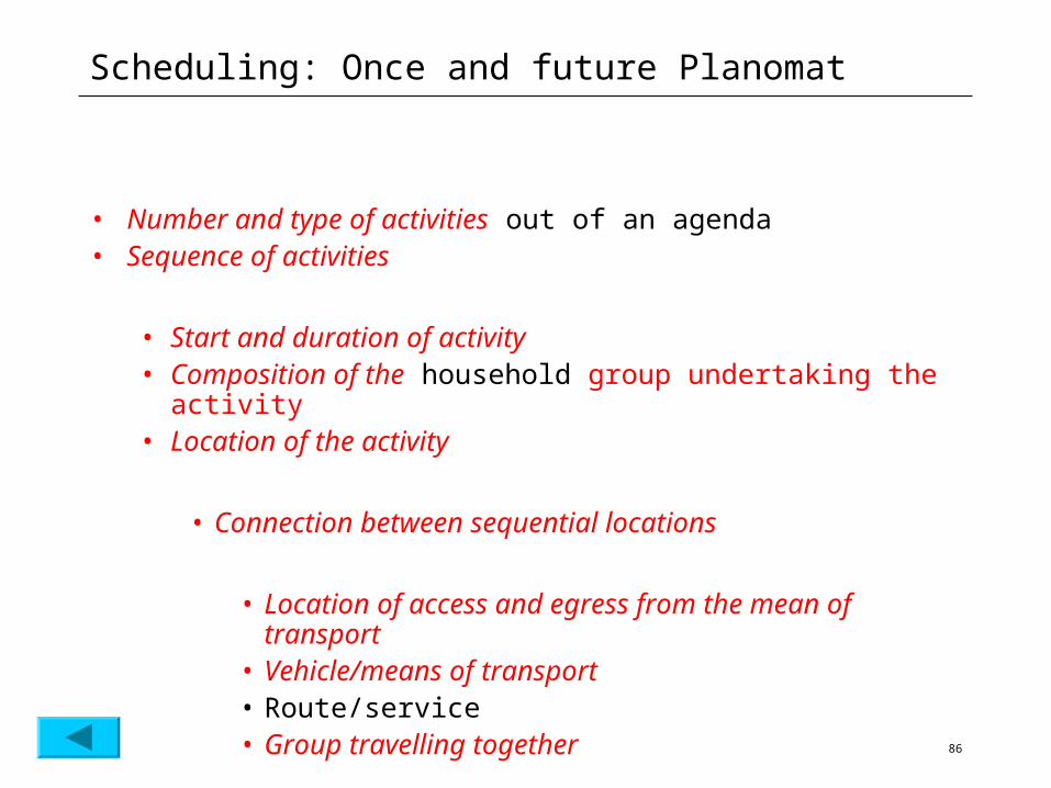
Scheduling: Once and future Planomat
• Number and type of activities out of an agenda• Sequence of activities
• Start and duration of activity• Composition of the household group undertaking the activity• Location of the activity
• Connection between sequential locations
• Location of access and egress from the mean of transport
• Vehicle/means of transport• Route/service• Group travelling together
87
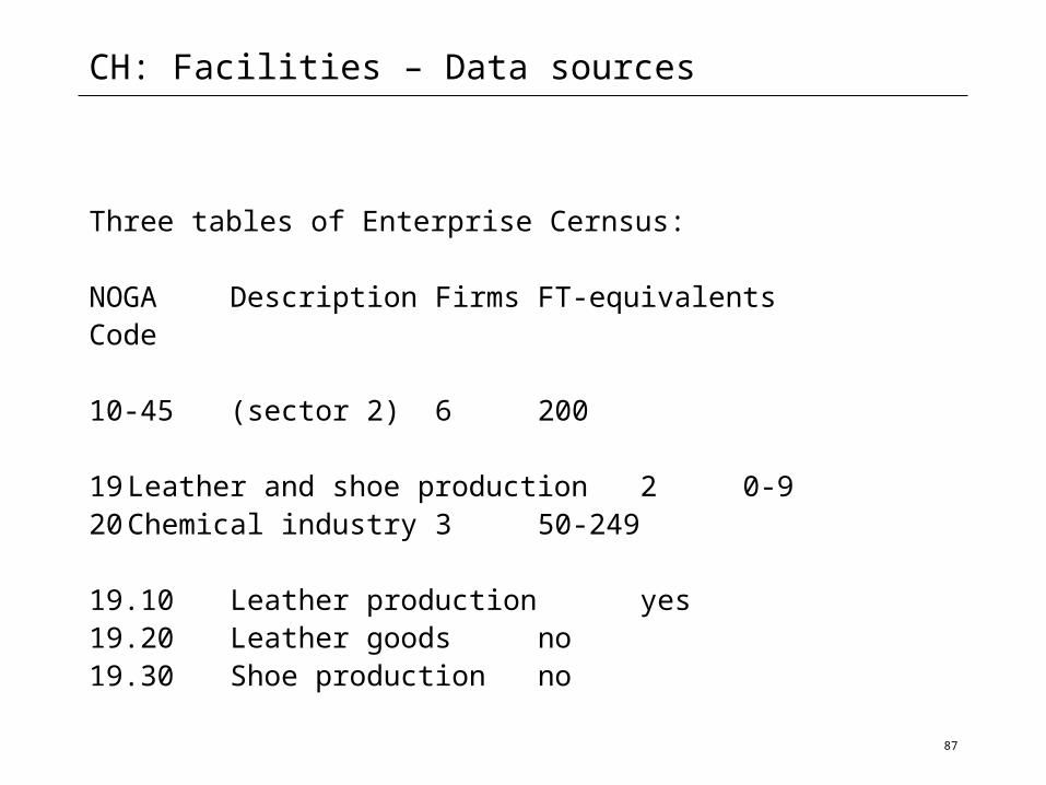
CH: Facilities – Data sources
Three tables of Enterprise Cernsus:
NOGA Description Firms FT-equivalentsCode
10-45 (sector 2) 6 200
19 Leather and shoe production 2 0-920 Chemical industry 3 50-249
19.10 Leather production yes19.20 Leather goods no19.30 Shoe production no
88
CH: Facilities – current allocation
• Read census of employment for each hectare
• Generate the required number of facilities
• Add activity work• Set number of work place to minimum of class• Distribute remainder proportionally to class size
• Add activity of use• Add standard opening hours• Randomly distribute on the hectare and attach to nearest
link
89
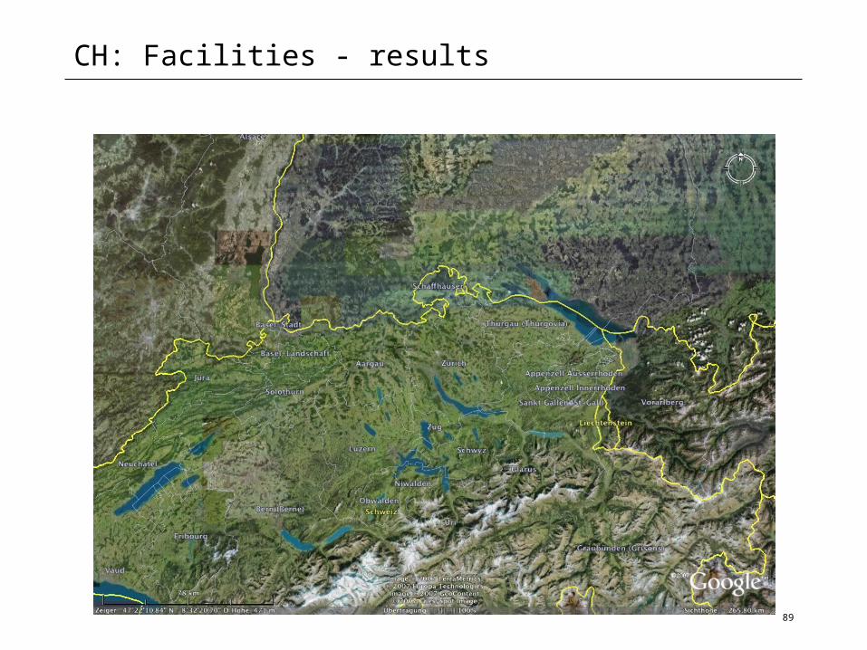
CH: Facilities - results
90
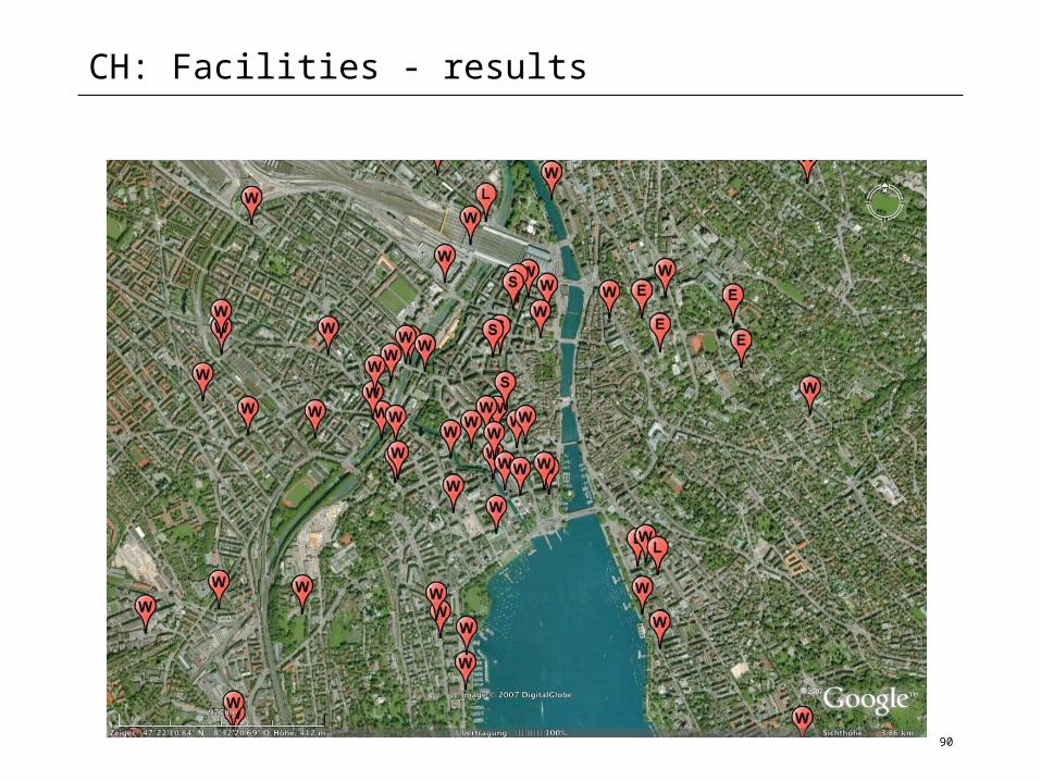
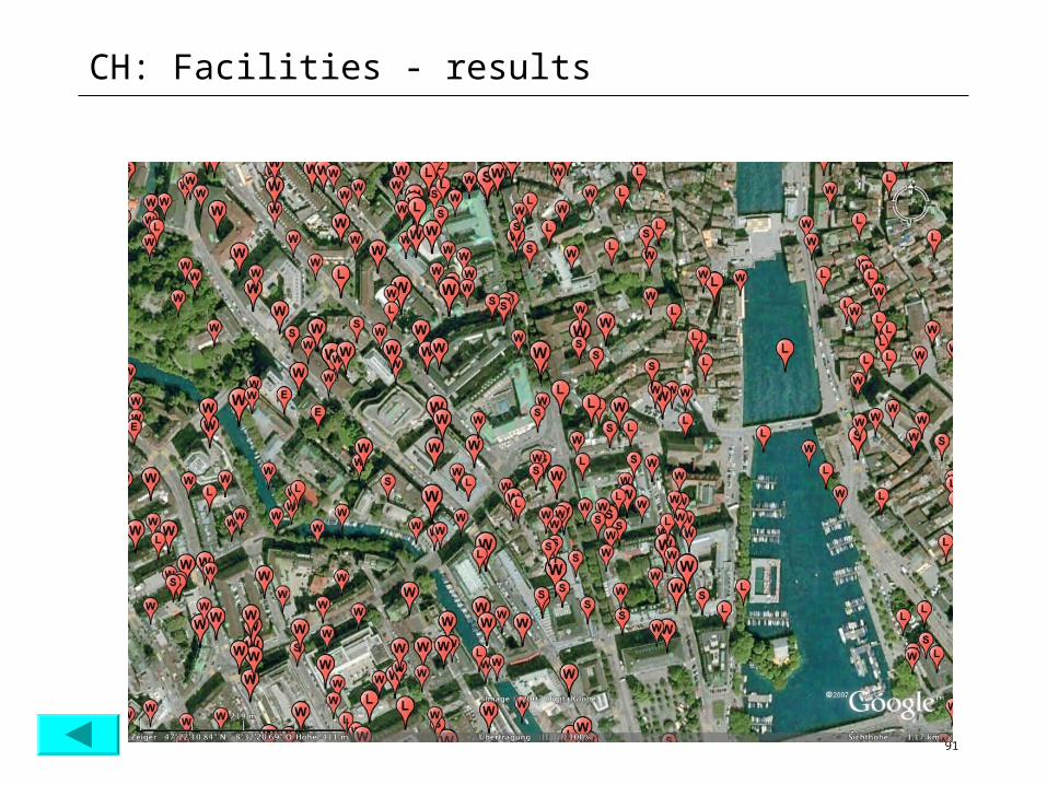
CH: Facilities - results
91
CH: Facilities - results