1 regeneration-based statistics for harris recurrent markov chains · 2016-03-14 · 1...

1

Regeneration-based statistics for Harrisrecurrent Markov chains

Patrice Bertail1 and Stephan Clemencon2

1 CREST-LS, 3, ave Pierre Larousse, 94205 Malakoff, [email protected]

2 MODAL’X - Universite Paris X NanterreLPMA - UMR CNRS 7599 - Universites Paris VI et Paris [email protected]

Abstract : Harris Markov chains make their appearance in many areas ofstatistical modeling, in particular in time series analysis. Recent years haveseen a rapid growth of statistical techniques adapted to data exhibiting thisparticular pattern of dependence. In this paper an attempt is made to presenthow renewal properties of Harris recurrent Markov chains or of specific exten-sions of the latter may be practically used for statistical inference in varioussettings. When the study of probabilistic properties of general Harris Markovchains may be classically carried out by using the regenerative method (cfSmith (1955)), via the theoretical construction of regenerative extensions (seeNummelin (1978)), statistical methodologies may also be based on regenera-tion for general Harris chains. In the regenerative case, such procedures areimplemented from data blocks corresponding to consecutive observed regener-ation times for the chain. And the main idea for extending the application ofthese statistical techniques to general Harris chains X consists in generatingfirst a sequence of approximate renewal times for a regenerative extension of Xfrom data X1, ..., Xn and the parameters of a minorization condition satisfiedby its transition probability kernel, and then applying the latter techniques tothe data blocks determined by these pseudo-regeneration times as if they wereexact regeneration blocks. Numerous applications of this estimation principlemay be considered in both the stationary and nonstationary (including thenull recurrent case) frameworks. This article deals with some important pro-cedures based on (approximate) regeneration data blocks, from both practicaland theoretical viewpoints, for the following topics: mean and variance esti-mation, confidence intervals, U -statistics, Bootstrap, robust estimation andstatistical study of extreme values.

2 Patrice Bertail and Stephan Clemencon

1.1 Introduction

1.1.1 On describing Markov chains via Renewal processes

Renewal theory plays a key role in the analysis of the asymptotic structureof many kinds of stochastic processes, and especially in the development ofasymptotic properties of general irreducible Markov chains. The underlyingground consists in the fact that limit theorems proved for sums of independentrandom vectors may be easily extended to regenerative random processes, thatis to say random processes that may be decomposed at random times, calledregeneration times, into a sequence of mutually independent blocks of obser-vations, namely regeneration cycles (see Smith (1955)). The method basedon this principle is traditionally called the regenerative method. Harris chainsthat possess an atom, i.e. a Harris set on which the transition probabilitykernel is constant, are special cases of regenerative processes and so directlyfall into the range of application of the regenerative method (Markov chainswith discrete state space as well as many markovian models widely used inoperational research for modeling storage or queuing systems are remarkableexamples of atomic chains). The theory developed in Nummelin (1978) (andin parallel the closely related concepts introduced in Athreya & Ney (1978))showed that general Markov chains could all be considered as regenerative ina broader sense (i.e. in the sense of the existence of a theoretical regenerativeextension for the chain, see § 2.3), as soon as the Harris recurrence propertyis satisfied. Hence this theory made the regenerative method applicable tothe whole class of Harris Markov chains and allowed to carry over many limittheorems to Harris chains such as LLN, CLT, LIL or Edgeworth expansions.

In many cases, parameters of interest for a Harris Markov chain may bethus expressed in terms of regeneration cycles. While, for atomic Markovchains, statistical inference procedures may be then based on a random num-ber of observed regeneration data blocks, in the general Harris recurrent casethe regeneration times are theoretical and their occurrence cannot be deter-mined by examination of the data only. Although the Nummelin splittingtechnique for constructing regeneration times has been introduced as a theo-retical tool for proving probabilistic results such as limit theorems or proba-bility and moment inequalities in the markovian framework, this article aimsto show that it is nevertheless possible to make a practical use of the latterfor extending regeneration-based statistical tools. Our proposal consists in anempirical method for building approximatively a realization drawn from aNummelin extension of the chain with a regeneration set and then recover-ing ”approximate regeneration data blocks”. As will be shown further, thoughthe implementation of the latter method requires some prior knowledge aboutthe behaviour of the chain and crucially relies on the computation of a con-sistent estimate of its transition kernel, this methodology allows for numerousstatistical applications.

We finally point out that, alternatively to regeneration-based statisticalmethods, inference techniques based on data (moving) blocks of fixed length

1 Regeneration-based statistics for Harris recurrent Markov chains 3

may also be used in our markovian framework. But as will be shown through-out the article, such blocking techniques, introduced for dealing with generaltime series (in the weakly dependent setting) are less powerful, when appliedto Harris Markov chains, than the methods we promote here, which are specif-ically tailored for (pseudo) regenerative processes.

1.1.2 Outline

The outline of the paper is as follows. In section 2, notations are set out andkey concepts of the Markov chain theory as well as some basic notions aboutthe regenerative method and the Nummelin splitting technique are recalled.Section 3 presents and discusses how to practically construct (approximate)regeneration data blocks, on which statistical procedures we investigate fur-ther are based. Sections 4 and 5 mainly survey results established at lengthin Bertail & Clemencon (2004a,b,c,d). More precisely, the problem of estima-ting additive functionals of the stationary distribution in the Harris positiverecurrent case is considered in section 4. Estimators based on the (pseudo)regenerative blocks, as well as estimates of their asymptotic variance are ex-hibited, and limit theorems describing the asymptotic behaviour of their biasand their sampling distribution are also displayed. Section 5 is devoted to thestudy of a specific resampling procedure, which crucially relies on the (ap-proximate) regeneration data blocks. Results proving the asymptotic validityof this particular bootstrap procedure (and its optimality regarding to secondorder properties in the atomic case) are stated. Section 6 shows how to ex-tend some of the results of sections 4 and 5 to V and U -statistics. A specificnotion of robustness for statistics based on the (approximate) regenerativeblocks is introduced and investigated in section 7. And asymptotic proper-ties of some regeneration-based statistics related to the extremal behaviourof Markov chains are studied in section 8 in the regenerative case only. Fi-nally, some concluding remarks are collected in section 9 and further lines ofresearch are sketched.

1.2 Theoretical background

1.2.1 Notation and definitions

We now set out the notations and recall a few definitions concerning the com-munication structure and the stochastic stability of Markov chains (for furtherdetail, refer to Revuz (1984) or Meyn & Tweedie (1996)). Let X = (Xn)n∈Nbe an aperiodic irreducible Markov chain on a countably generated state space(E, E), with transition probability Π, and initial probability distribution ν.For any B ∈ E and any n ∈ N, we thus have

X0 ∼ ν and P(Xn+1 ∈ B | X0, ..., Xn) = Π(Xn, B) a.s. .


In what follows, Pν (respectively Px for x in E) will denote the probabilitymeasure on the underlying probability space such that X0 ∼ ν (resp. X0 = x),Eν (.) the Pν-expectation (resp. Ex (.) the Px-expectation), I{A} will denotethe indicator function of the event A and ⇒ the convergence in distribution.

A measurable set B is Harris recurrent for the chain if for any x ∈ B,Px(

∑∞n=1 I{Xn ∈ B} = ∞) = 1. The chain is said Harris recurrent if it

is ψ-irreducible and every measurable set B such that ψ(B) > 0 is Harrisrecurrent. When the chain is Harris recurrent, we have the property thatPx(

∑∞n=1 I{Xn ∈ B} = ∞) = 1 for any x ∈ E and any B ∈ E such that

ψ(B) > 0.A probability measure µ on E is said invariant for the chain when µΠ = µ,

where µΠ(dy) =∫

x∈Eµ(dx)Π (x, dy). An irreducible chain is said positive

recurrent when it admits an invariant probability (it is then unique).Now we recall some basics concerning the regenerative method and its

application to the analysis of the behaviour of general Harris chains via theNummelin splitting technique (refer to Nummelin (1984) for further detail).

1.2.2 Markov chains with an atom

Assume that the chain is ψ-irreducible and possesses an accessible atom, thatis to say a measurable set A such that ψ(A) > 0 and Π(x, .) = Π(y, .) for allx, y in A. Denote by τA = τA(1) = inf {n ≥ 1, Xn ∈ A} the hitting time on A,by τA(j) = inf {n > τA(j − 1), Xn ∈ A} for j ≥ 2 the successive return timesto A and by EA (.) the expectation conditioned on X0 ∈ A. Assume furtherthat the chain is Harris recurrent, the probability of returning infinitely oftento the atom A is thus equal to one, no matter what the starting point. Then,it follows from the strong Markov property that, for any initial distributionν, the sample paths of the chain may be divided into i.i.d. blocks of randomlength corresponding to consecutive visits to A:

B1 = (XτA(1)+1, ..., XτA(2)), ..., Bj = (XτA(j)+1, ..., XτA(j+1)), ...

taking their values in the torus T = ∪∞n=1En. The sequence (τA(j))j>1 de-

fines successive times at which the chain forgets its past, called regenerationtimes. We point out that the class of atomic Markov chains contains not onlychains with a countable state space (for the latter, any recurrent state is anaccessible atom), but also many specific Markov models arising from the fieldof operational research (see Asmussen (1987) for regenerative models involvedin queuing theory, as well as the examples given in § 4.3). When an accessibleatom exists, the stochastic stability properties of the chain amount to proper-ties concerning the speed of return time to the atom only. For instance, in thisframework, the following result, known as Kac’s theorem, holds (cf Theorem10.2.2 in Meyn & Tweedie (1996)).

Theorem 1. The chain X is positive recurrent iff EA(τA) < ∞. The (unique)invariant probability distribution µ is then the Pitman’s occupation measuregiven by


µ(B) = EA(τA∑

i=1

I{Xi ∈ B})/EA(τA), for all B ∈ E .

For atomic chains, limit theorems can be derived from the applicationof the corresponding results to the i.i.d. blocks (Bn)n>1. One may refer forexample to Meyn & Tweedie (1996) for the LLN, CLT, LIL, Bolthausen(1980) for the Berry-Esseen theorem, Malinovskii (1985, 87, 89) and Bertail& Clemencon (2004a) for other refinements of the CLT. The same techniquecan also be applied to establish moment and probability inequalities, whichare not asymptotic results (see Clemencon (2001)). As mentioned above, theseresults are established from hypotheses related to the distribution of the Bn’s.The following assumptions shall be involved throughout the article. Let κ > 0,f : E → R be a measurable function and ν be a probability distribution on(E, E).

Regularity conditions:

H0(κ) : EA(τκA) < ∞,

H0(κ, ν) : Eν(τκA) < ∞.

Block-moment conditions:

H1(κ, f) : EA((τA∑

i=1

|f(Xi)|)κ) < ∞,

H1(κ, ν, f) : Eν((τA∑

i=1

|f(Xi)|)κ) < ∞.

Remark 1. We point out that conditions H0(κ) and H1(κ, f) do not dependon the accessible atom chosen : if they hold for a given accessible atom A,they are also fulfilled for any other accessible atom (see Chapter 11 in Meyn& Tweedie (1996)). Besides, the relationship between the ”block moment”conditions and the rate of decay of mixing coefficients has been investigatedin Bolthausen (1982): for instance, H0(κ) (as well as H1(κ, f) when f isbounded) is typically fulfilled as soon as the strong mixing coefficients se-quence decreases at an arithmetic rate n−ρ, for some ρ > κ− 1.

1.2.3 General Harris recurrent chains

The Nummelin splitting technique

We now recall the splitting technique introduced in Nummelin (1978) for ex-tending the probabilistic structure of the chain in order to construct an ar-tificial regeneration set in the general Harris recurrent case. It relies on thecrucial notion of small set. Recall that, for a Markov chain valued in a statespace (E, E) with transition probability Π, a set S ∈ E is said to be small if


there exist m ∈ N∗, δ > 0 and a probability measure Γ supported by S suchthat, for all x ∈ S, B ∈ E ,

Πm(x,B) ≥ δΓ (B), (1.1)

denoting by Πm the m-th iterate of Π. When this holds, we say that thechain satisfies the minorization condition M(m,S, δ, Γ ). We emphasize thataccessible small sets always exist for ψ-irreducible chains: any set B ∈ E suchthat ψ(B) > 0 actually contains such a set (cf Jain & Jamison (1967)). Nowlet us precise how to construct the atomic chain onto which the initial chain Xis embedded, from a set on which an iterate Πm of the transition probabilityis uniformly bounded below. Suppose that X satisfies M = M(m,S, δ, Γ ) forS ∈ E such that ψ(S) > 0. Even if it entails replacing the chain (Xn)n∈N bythe chain

((Xnm, ..., Xn(m+1)−1

))n∈N, we suppose m = 1. The sample space

is expanded so as to define a sequence (Yn)n∈N of independent Bernoulli r.v.’swith parameter δ by defining the joint distribution Pν,M whose constructionrelies on the following randomization of the transition probability Π each timethe chain hits S (note that it happens a.s. since the chain is Harris recurrentand ψ(S) > 0). If Xn ∈ S and

• if Yn = 1 (which happens with probability δ ∈ ]0, 1[), then Xn+1 is dis-tributed according to Γ ,

• if Yn = 0, (which happens with probability 1 − δ), then Xn+1 is drawnfrom (1− δ)−1(Π(Xn+1, .)− δΓ (.)).

Set Berδ(β) = δβ+(1−δ)(1−β) for β ∈ {0, 1}. We now have constructed abivariate chain XM = ((Xn, Yn))n∈N , called the split chain, taking its valuesin E × {0, 1} with transition kernel ΠM defined by

• for any x /∈ S, B ∈ E , β and β′ in {0, 1} ,

ΠM ((x, β) , B × {β′}) = Berδ(β′)×Π (x, B) ,

• for any x ∈ S, B ∈ E , β′ in {0, 1} ,

ΠM ((x, 1) , B × {β′}) = Berδ(β′)× Γ (B),

ΠM ((x, 0) , A× {β′}) = Berδ(β′)× (1− δ)−1(Π (x,B)− δΓ (B)).

Basic assumptions

The whole point of the construction consists in the fact that S×{1} is an atomfor the split chain XM, which inherits all the communication and stochasticstability properties from X (irreducibility, Harris recurrence,...), in partic-ular (for the case m = 1 here) the blocks constructed for the split chainare independent. Hence the splitting method enables to extend the regener-ative method, and so to establish all of the results known for atomic chains,


to general Harris chains. It should be noticed that if the chain X satisfiesM(m,S, δ, Γ ) for m > 1, the resulting blocks are not independent anymorebut 1-dependent, a form of dependence which may be also easily handled. Forsimplicity ’s sake, we suppose in what follows that condition M is fulfilledwith m = 1, we shall also omit the subscript M and abusively denote byPν the extensions of the underlying probability we consider. The followingassumptions, involving the speed of return to the small set S shall be usedthroughout the article. Let κ > 0, f : E → R be a measurable function and νbe a probability measure on (E, E).

Regularity conditions:

H′0(κ) : supx∈S

Ex(τκS ) < ∞,

H′0(κ, ν) : Eν(τκS ) < ∞.

Block-moment conditions:

H′1(κ, f) : supx∈S

Ex((τS∑

i=1

|f(Xi)|)κ) < ∞,

H′1(κ, f, ν) : Eν((τS∑

i=1

|f(Xi)|)κ) < ∞.

Remark 2. It is noteworthy that assumptions H′0(κ) and H′1(κ, f) do not de-pend on the choice of the small set S (if they are checked for some accessiblesmall set S, they are fulfilled for all accessible small sets cf § 11.1 in Meyn& Tweedie (1996)). Note also that in the case when H′0(κ) (resp. H′0(κ, ν))is satisfied, H′1(κ, f) (resp., H′1(κ, f, ν)) is fulfilled for any bounded f . More-over, recall that positive recurrence, conditions H′1(κ) and H′1(κ, f) may bepractically checked by using test functions methods (cf Kalashnikov (1978),Tjøstheim (1990)). In particular, it is well known that such block momentassumptions may be replaced by drift criteria of Lyapounov’s type (refer toChapter 11 in Meyn & Tweedie (1996) for further details on such conditionsand many illustrating examples, see also Douc et al. (2004)).

We recall finally that such assumptions on the initial chain classically implythe desired conditions for the split chain: as soon as X fulfills H′0(κ) (resp.,H′0(κ, ν), H′1(κ, f), H′1(κ, f, ν)), XM satisfies H0(κ) (resp., H0(κ, ν), H1(κ,f), H1(κ, f, ν)).

The distribution of (Y1, ..., Yn) conditioned on (X1, ..., Xn+1).

As will be shown in the next section, the statistical methodology for Har-ris chains we propose is based on approximating the conditional distribu-tion of the binary sequence (Y1, ..., Yn) given X(n+1) = (X1, ..., Xn+1). We


thus precise the latter. Let us assume further that the family of the condi-tional distributions {Π(x, dy)}x∈E and the initial distribution ν are domi-nated by a σ-finite measure λ of reference, so that ν(dy) = f(y)λ(dy) andΠ(x, dy) = p(x, y)λ(dy), for all x ∈ E. Notice that the minorization conditionentails that Γ is absolutely continuous with respect to λ too, and that

p(x, y) ≥ δγ(y), λ(dy) a.s. (1.2)

for any x ∈ S, with Γ (dy) = γ(y)dy. The distribution of Y (n) = (Y1, ...,Yn) conditionally to X(n+1) = (x1, ..., xn+1) is then the tensor product ofBernoulli distributions given by: for all β(n) = (β1, ..., βn) ∈ {0, 1}n

, x(n+1) =(x1, ..., xn+1) ∈ En+1,

Pν

(Y (n) = β(n) | X(n+1) = x(n+1)

)=

n∏

i=1

Pν(Yi = βi | Xi = xi, Xi+1 = xi+1),

with, for 1 6 i 6 n,

Pν(Yi = 1 | Xi = xi, Xi+1 = xi+1) = δ, if xi /∈ S,

Pν(Yi = 1 | Xi = xi, Xi+1 = xi+1) =δγ(xi+1)

p(xi, xi+1), if xi ∈ S.

Roughly speaking, conditioned on X(n+1), from i = 1 to n, Yi is drawnfrom the Bernoulli distribution with parameter δ, unless X has hit the smallset S at time i: in this case Yi is drawn from the Bernoulli distribution with pa-rameter δγ(Xi+1)/p(Xi, Xi+1). We denote by L(n)(p, S, δ, γ, x(n+1)) this prob-ability distribution.

1.3 Dividing the sample path into (approximate)regeneration cycles

In the preceding section, we recalled the Nummelin approach for the theoret-ical construction of regeneration times in the Harris framework. Here we nowconsider the problem of approximating these random times from data setsin practice and propose a basic preprocessing technique, on which estimationmethods we shall discuss further are based.

1.3.1 Regenerative case

Let us suppose we observed a trajectory X1, ..., Xn of length n drawn fromthe chain X. In the regenerative case, when an atom A for the chain is a prioriknown, regeneration blocks are naturally obtained by simply examining thedata, as follows.

Algorithm 1 (Regeneration blocks construction)


1. Count the number of visits ln =∑n

i=1 I{Xi ∈ A} to A up to time n.2. Divide the observed trajectory X(n) = (X1, ...., Xn) into ln + 1 blocks

corresponding to the pieces of the sample path between consecutive visitsto the atom A,

B0 = (X1, ..., XτA(1)), B1 = (XτA(1)+1, ..., XτA(2)), ...,

Bln−1 = (XτA(ln−1)+1, ..., XτA(ln)), B(n)ln

= (XτA(ln)+1, ..., Xn),

with the convention B(n)ln

= ∅ when τA(ln) = n.

3. Drop the first block B0, as well as the last one B(n)ln

, when non-regenerative(i.e. when τA(ln) < n).

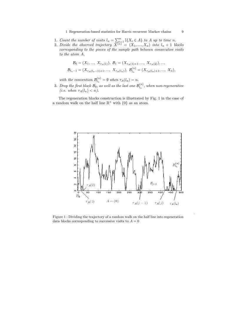
The regeneration blocks construction is illustrated by Fig. 1 in the case ofa random walk on the half line R+ with {0} as an atom.

Figure 1 : Dividing the trajectory of a random walk on the half line into regenerationdata blocks corresponding to successive visits to A = 0


1.3.2 General Harris case

The principle

Suppose now that observations X1, ..., Xn+1 are drawn from a Harris chainX satisfying the assumptions of § 2.3.3 (refer to the latter paragraph forthe notations). If we were able to generate binary data Y1, ..., Yn, so thatXM (n) = ((X1, Y1), ..., (Xn, Yn)) be a realization of the split chain XM de-scribed in § 2.3, then we could apply the regeneration blocks constructionprocedure to the sample path XM (n). Unfortunately, knowledge of the tran-sition density p(x, y) for (x, y) ∈ S2 is required to draw practically the Yi’sthis way. We propose a method relying on a preliminary estimation of the”nuisance parameter” p(x, y). More precisely, it consists in approximatingthe splitting construction by computing an estimator pn(x, y) of p(x, y) usingdata X1, ..., Xn+1, and to generate a random vector (Y1, ..., Yn) conditionallyto X(n+1) = (X1, ..., Xn+1), from distribution L(n)(pn, S, δ, γ,X(n+1)), whichapproximates in some sense the conditional distribution L(n)(p, S, δ, γ, X(n+1))of (Y1, ..., Yn) for given X(n+1). Our method, which we call approximate regen-eration blocks construction (ARB construction in abbreviated form) amountsthen to apply the regeneration blocks construction procedure to the data((X1, Y1), ..., (Xn, Yn)) as if they were drawn from the atomic chain XM. Inspite of the necessary consistent transition density estimation step, we shallshow in the sequel that many statistical procedures, that would be consis-tent in the ideal case when they would be based on the regeneration blocks,remain asymptotically valid when implemented from the approximate datablocks. For given parameters (δ, S, γ) (see § 3.2.2 for a data driven choiceof these parameters), the approximate regeneration blocks are constructed asfollows.

Algorithm 2 (Approximate regeneration blocks construction)

1. From the data X(n+1) = (X1, ..., Xn+1), compute an estimate pn(x, y)of the transition density such that pn(x, y) ≥ δγ(y), λ(dy) a.s., andpn(Xi, Xi+1) > 0, 1 6 i 6 n.

2. Conditioned on X(n+1), draw a binary vector (Y1, ..., Yn) from the dis-tribution estimate L(n)(pn, S, δ, γ, X(n+1)). It is sufficient in practice todraw the Yi’s at time points i when the chain visits the set S (i.e. whenXi ∈ S), since at these times and at these times only the split chain mayregenerate. At such a time point i, draw Yi according to the Bernoullidistribution with parameter δγ(Xi+1)/pn(Xi, Xi+1)).

3. Count the number of visits ln =∑n

i=1 I{Xi ∈ S, Yi = 1) to the setAM = S × {1} up to time n and divide the trajectory X(n+1) into ln + 1approximate regeneration blocks corresponding to the successive visits of(X, Y ) to AM,


B0 = (X1, ..., XbτAM (1)), B1 = (XbτAM (1)+1, ..., XbτAM (2)), ...,

Bbln−1 = (XbτAM (bln−1)+1, ..., XbτAM (bln)), B(n)ln

= (XbτAM (bln)+1, ..., Xn+1),

where τAM(1) = inf{n > 1, Xn ∈ S, Yn = 1} and τAM(j + 1) = inf{n >

τAM(j), Xn ∈ S, Yn = 1} for j > 1.

4. Drop the first block B0 and the last one B(n)ln

when τAM(ln) < n.

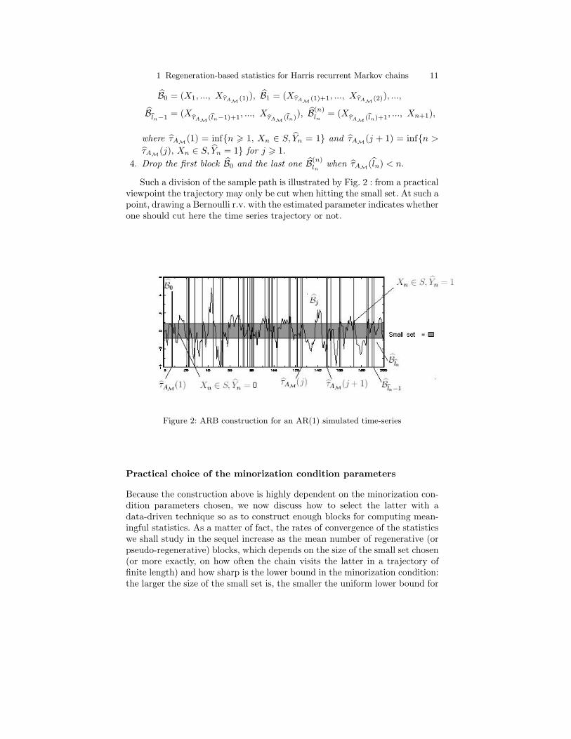
Such a division of the sample path is illustrated by Fig. 2 : from a practicalviewpoint the trajectory may only be cut when hitting the small set. At such apoint, drawing a Bernoulli r.v. with the estimated parameter indicates whetherone should cut here the time series trajectory or not.

Figure 2: ARB construction for an AR(1) simulated time-series

Practical choice of the minorization condition parameters

Because the construction above is highly dependent on the minorization con-dition parameters chosen, we now discuss how to select the latter with adata-driven technique so as to construct enough blocks for computing mean-ingful statistics. As a matter of fact, the rates of convergence of the statisticswe shall study in the sequel increase as the mean number of regenerative (orpseudo-regenerative) blocks, which depends on the size of the small set chosen(or more exactly, on how often the chain visits the latter in a trajectory offinite length) and how sharp is the lower bound in the minorization condition:the larger the size of the small set is, the smaller the uniform lower bound for


the transition density. This leads us to the following trade-off. Roughly speak-ing, for a given realization of the trajectory, as one increases the size of thesmall set S used for the data blocks construction, one naturally increases thenumber of points of the trajectory that are candidates for determining a block(i.e. a cut in the trajectory), but one also decreases the probability of cut-ting the trajectory (since the uniform lower bound for {p(x, y)}(x,y)∈S2 thendecreases). This gives an insight into the fact that better numerical resultsfor statistical procedures based on the ARB construction may be obtainedin practice for some specific choices of the small set, likely for choices corre-sponding to a maximum expected number of data blocks given the trajectory,that is

Nn(S) = Eν(n∑

i=1

I{Xi ∈ S, Yi = 1} |X(n+1)).

Hence, when no prior information about the structure of the chain is avail-able, here is a practical data-driven method for selecting the minorizationcondition parameters in the case when the chain takes real values. Con-sider a collection S of borelian sets S (typically compact intervals) anddenote by US(dy) = γS(y).λ(dy) the uniform distribution on S, whereγS(y) = I{y ∈ S}/λ(S) and λ is the Lebesgue measure on R. Now, forany S ∈ S, set δ(S) = λ(S). inf(x,y)∈S2 p(x, y). We have for any x, y in S,p(x, y) ≥ δ(S)γS(y). In the case when δ(S) > 0, the ideal criterion to opti-mize may be then expressed as

Nn(S) =δ(S)λ(S)

n∑

i=1

I{(Xi, Xi+1) ∈ S2}p(Xi, Xi+1)

. (1.3)

However, as the transition kernel p(x, y) and its minimum over S2 are un-known, a practical empirical criterion is obtained by replacing p(x, y) byan estimate pn(x, y) and δ(S) by a lower bound δn(S) for λ(S).pn(x, y)over S2 in expression (1.3). Once pn(x, y) is computed, calculate δn(S) =λ(S). inf(x,y)∈S2 pn(x, y) and maximize thus the empirical criterion over S ∈ S

Nn(S) =δn(S)λ(S)

n∑

i=1

I{(Xi, Xi+1) ∈ S2}pn(Xi, Xi+1)

. (1.4)

More specifically, one may easily check at hand on many examples of realvalued chains (see § 4.3 for instance), that any compact interval Vx0(ε) = [x0−ε, x0 + ε] for some well chosen x0 ∈ R and ε > 0 small enough, is a small set,choosing γ as the density of the uniform distribution on Vx0(ε). For practicalpurpose, one may fix x0 and perform the optimization over ε > 0 only (seeBertail & Clemencon (2004c)) but both x0 and ε may be considered as tuningparameters. A possible numerically feasible selection rule could rely then onsearching for (x0, ε) on a given pre-selected grid G = {(x0(k), ε(l)), 1 6 k 6 K,1 6 l 6 L} such that inf(x,y)∈Vx0 (ε)2 pn(x, y) > 0 for any (x0, ε) ∈ G.

Algorithm 3 (ARB construction with empirical choice of the small set)


1. Compute an estimator pn(x, y) of p(x, y).2. For any (x0, ε) ∈ G, compute the estimated expected number of pseudo-

regenerations:

Nn(x0, ε) =δn(x0, ε)

2ε

n∑

i=1

I{(Xi, Xi+1) ∈ Vx0(ε)2}

pn(Xi, Xi+1),

with δn(x0, ε) = 2ε. inf(x,y)∈Vx0 (ε)2 pn(x, y).3. Pick (x∗0, ε

∗) in G maximizing Nn(x0, ε) over G, corresponding to the setS∗ = [x∗0 − ε∗, x∗0 + ε∗] and the minorization constant δ∗n = δn(x∗0, ε

∗).4. Apply Algorithm 2 for ARB construction using S∗, δ∗n and pn.

Remark 3. Numerous consistent estimators of the transition density of Harrischains have been proposed in the literature. Refer to Roussas (1969, 91a,91b), Rosenblatt (1970), Birge (1983), Doukhan & Ghindes (1983), PrakasaRao (1983), Athreya & Atuncar (1998) or Clemencon (2000) for instance inpositive recurrent cases, Karlsen & Tjøstheim (2001) in specific null recurrentcases.

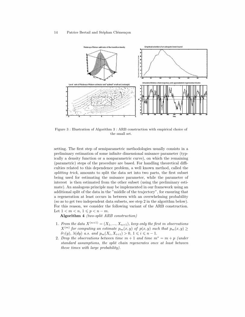
This method is illustrated by Fig. 3 in the case of an AR(1) model: Xi+1 =αXi + εi+1, i ∈ N, with εi

i.i.d.∼ N (0, 1), α = 0.95 and X0 = 0, for a trajectoryof length n = 200. Taking x0 = 0 and letting ε grow, the expected numberregeneration blocks is maximum for ε∗ close to 0.9. The true minimum value ofp(x, y) over the corresponding square is actually δ = 0.118. The first graphicin this panel shows the Nadaraya-Watson estimator

pn(x, y) =∑n

i=1 K(h−1(x−Xi))K(h−1(y −Xi+1))∑ni=1 K(h−1(x−Xi))

,

computed from the gaussian kernel K(x) = (2π)−1 exp(−x2/2) with an opti-mal bandwidth h of order n−1/5. The second one plots Nn(ε) as a function ofε. The next one indicates the set S∗ corresponding to our empirical selectionrule, while the last one displays the ”optimal” ARB construction.

Note finally that other approaches may be considered for determining prac-tically small sets and establishing accurate minorization conditions, whichconditions do not necessarily involve uniform distributions besides. Refer forinstance to Roberts & Rosenthal (1996) for Markov diffusion processes.

A two-split version of the ARB construction

When carrying out the theoretical study of statistical methods based on theARB construction, one must deal with difficult problems arising from thedependence structure in the set of the resulting data blocks, due to the pre-liminary estimation step. Such difficulties are somehow similar as the onesthat one traditionally faces in a semiparametric framework, even in the i.i.d.


Figure 3 : Illustration of Algorithm 3 : ARB construction with empirical choice ofthe small set.

setting. The first step of semiparametric methodologies usually consists in apreliminary estimation of some infinite dimensional nuisance parameter (typ-ically a density function or a nonparametric curve), on which the remaining(parametric) steps of the procedure are based. For handling theoretical diffi-culties related to this dependence problem, a well known method, called thesplitting trick, amounts to split the data set into two parts, the first subsetbeing used for estimating the nuisance parameter, while the parameter ofinterest is then estimated from the other subset (using the preliminary esti-mate). An analogous principle may be implemented in our framework using anadditional split of the data in the ”middle of the trajectory”, for ensuring thata regeneration at least occurs in between with an overwhelming probability(so as to get two independent data subsets, see step 2 in the algorithm below).For this reason, we consider the following variant of the ARB construction.Let 1 < m < n, 1 6 p < n−m.

Algorithm 4 (two-split ARB construction)

1. From the data X(n+1) = (X1, ..., Xn+1), keep only the first m observationsX(m) for computing an estimate pm(x, y) of p(x, y) such that pm(x, y) ≥δγ(y), λ(dy) a.s. and pm(Xi, Xi+1) > 0, 1 6 i 6 n− 1.

2. Drop the observations between time m + 1 and time m∗ = m + p (understandard assumptions, the split chain regenerates once at least betweenthese times with large probability).


3. From remaining observations X(m∗,n) = (Xm∗+1, ..., Xn) and estimatepm, apply steps 2-4 of Algorithm 2 (respectively of Algorithm 3).

This procedure is similar to the 2-split method proposed in Schick (2001),except that here the number of deleted observations is arbitrary and easierto interpret in term of regeneration. Of course, the more often the split chainregenerates, the smaller p may be chosen. And the main problem consists inpicking m = mn so that mn →∞ as n →∞ for the estimate of the transitionkernel to be accurate enough, while keeping enough observation n−m∗ for theblock construction step: one typically chooses m = o(n) as n → ∞. Furtherassumptions are required for investigating precisely how to select m. In Bertail& Clemencon (2004d), a choice based on the rate of convergence αm of theestimator pm(x, y) (for the MSE when error is measured by the sup-normover S×S, see assumption H2 in § 4.2) is proposed: when considering smoothmarkovian models for instance, estimators with rate αm = m−1 log(m) maybe exhibited and one shows that m = n2/3 is then an optimal choice (up toa log(n)). However, one may argue, as in the semiparametric case, that thismethodology is motivated by our limitations in the analysis of asymptoticproperties of the estimators only, whereas from a practical viewpoint it maydeteriorate the finite sample performance of the initial algorithm. To our ownexperience, it is actually better to construct the estimate p(x, y) from thewhole trajectory and the interest of Algorithm 4 is mainly theoretical.

1.4 Mean and variance estimation

In this section, we suppose that the chain X is positive recurrent with un-known stationary probability µ and consider the problem of estimating anadditive functional of type µ(f) =

∫f(x)µ(dx) = Eµ(f(X1)), where f is a

µ-integrable real valued function defined on the state space (E, E). Estima-tion of additive functionals of type Eµ(F (X1, ..., Xk)), for fixed k > 1, maybe investigated in a similar fashion. We set f(x) = f(x)− µ(f).


Here we assume further that X admits an a priori known accessible atomA. As in the i.i.d. setting, a natural estimator of µ(f) is the sample meanstatistic,

µ′n(f) = n−1n∑

i=1

f(Xi). (1.5)

When the chain is stationary (i.e. when ν = µ), the estimator µ′n(f) haszero-bias. However, its bias is significant in all other cases, mainly because ofthe presence of the first and last (non-regenerative) data blocks B0 and B(n)

ln


(see Proposition 4.1 below). Besides, by virtue of Theorem 2.1, µ(f) may beexpressed as the mean of the f(Xi)’s over a regeneration cycle (renormalizedby the mean length of a regeneration cycle)

µ(f) = EA(τA)−1EA(τA∑

i=1

f(Xi)).

This suggests to introduce the following estimators of the mean µ(f). Definethe sample mean based on the observations (eventually) collected after thefirst regeneration time only by µn(f) = (n − τA)−1

∑ni=1+τA

f(Xi) with theconvention µn(f) = 0, when τA > n, as well as the sample mean based on theobservations collected between the first and last regeneration times before n

by µn(f) = (τA(ln) − τA)−1∑τA(ln)

i=1+τAf(Xi) with ln =

∑ni=1 I{Xi ∈ A} and

the convention µn(f) = 0, when ln 6 1 (observe that, by Markov’s inequality,Pν(ln 6 1) = O(n−1) as n →∞, as soon as H0(1, ν) and H0(2) are fulfilled).

Let us introduce some additional notation for the block sums (resp. theblock lengths), that shall be used here and throughout. For j > 1, n > 1, set

l(B0) = τA, l(Bj) = τA(j + 1)− τA(j), l(B(n)ln

) = n− τA(ln)

for the length of the blocks and

f(B0) =τA∑

i=1

f(Xi), f(Bj) =τA(j+1)∑

i=1+τA(j)

f(Xi), f(B(n)ln

) =n∑

i=1+τA(ln)

f(Xi)

for the value of the functional on the blocks. With these notations, the esti-mators above may be rewritten as

µ′n(f) =f(B0) +

∑ln−1j=1 f(Bj) + f(B(n)

ln)

l(B0) +∑ln−1

j=1 l(Bj) + l(B(n)ln

),

µn(f) =

∑ln−1j=1 f(Bj) + f(B(n)

ln)

∑ln−1j=1 l(Bj) + l(B(n)

ln)

, µn(f) =

∑ln−1j=1 f(Bj)∑ln−1j=1 l(Bj)

.

Let µn(f) designs any of the three estimators µ′n(f), µn(f) or µn(f). If Xfulfills conditions H0(2), H0(2, ν), H1(f, 2, A), H1(f, 2, ν) then the followingCLT holds under Pν (cf Theorem 17.2.2 in Meyn & Tweedie (1996))

n1/2σ−1(f)(µn(f)− µ(f)) ⇒ N (0, 1) , as n →∞,

with a normalizing constant

σ2(f) = µ (A)EA((τA∑

i=1

f(Xi)− µ(f)τA)2), (1.6)


From this expression we propose the following estimator of the asymptoticvariance, adopting the usual convention regarding to empty summation,

σ2n(f) = n−1

ln−1∑

j=1

(f(Bj)− µn(f)l(Bj))2. (1.7)

Notice that the first and last data blocks are not involved in its construction.We could have proposed estimators involving different estimates of µ(f), butas will be seen later, it is preferable to consider an estimator based on regener-ation blocks only. The following quantities shall be involved in the statisticalanalysis below. Define

α = EA(τA), β = EA(τA

τA∑

i=1

f(Xi)) = CovA(τA,

τA∑

i=1

f(Xi)),

ϕν = Eν(τA∑

i=1

f(Xi)), γ = α−1EA(τA∑

i=1

(τA − i)f(Xi)).

We also introduce the following technical conditions.(C1) (Cramer condition)

limt→∞

| EA(exp(itτA∑

i=1

f(Xi))) |< 1.

(C2) (Cramer condition)

limt→∞

| EA(exp(it(τA∑

i=1

f(Xi))2)) |< 1.

(C3) There exists N > 1 such that the N -fold convoluted density g∗N isbounded, denoting by g the density of the (

∑τA(j+1)i=1+τA(j) f(Xi) − α−1β)2’s.

(C4) There exists N > 1 such that the N -fold convoluted density G∗N isbounded, denoting by G the density of the (

∑τA(j+1)i=1+τA(j) f(Xi))2’s.

These two conditions are automatically satisfied if∑τA(2)

i=1+τA(1) f(Xi) hasa bounded density.

The result below is a straightforward extension of Theorem 1 in Mali-novskii (1985)(see also Proposition 3.1 in Bertail & Clemencon (2004a)).

Proposition 1. Suppose that H0(4), H0(2, ν), H1(4, f), H1(2, ν, f) andCramer condition (C1) are satisfied by the chain. Then, as n →∞, we have

Eν(µ′n(f)) = µ(f) + (ϕν + γ − β/α)n−1 + O(n−3/2), (1.8)

Eν(µn(f)) = µ(f) + (γ − β/α)n−1 + O(n−3/2), (1.9)

Eν(µn(f)) = µ(f)− (β/α)n−1 + O(n−3/2). (1.10)


If the Cramer condition (C2) is also fulfilled, then

Eν(σ2n(f)) = σ2(f) + O(n−1), as n →∞, (1.11)

and we have the following CLT under Pν ,

n1/2(σ2n(f)− σ2(f)) ⇒ N (0, ξ2(f)), as n →∞, (1.12)

with ξ2(f) = µ(A)V arA((∑τA

i=1 f(Xi))2 − 2α−1β∑τA

i=1 f(Xi)).

Proof. The proof of (1.8)-(1.11) is given in Bertail & Clemencon (2004a) andthe linearization of σ2

n(f) below follows from their Lemma 6.3

σ2n(f) = n−1

ln−1∑

j=1

g(Bj) + rn, (1.13)

with g(Bj) = f(Bj)2− 2α−1βf(Bj), for j > 1, and for some η1 > 0, Pν(nrn >η1 log(n)) = O(n−1), as n →∞. We thus have, as n →∞,

n1/2(σ2n(f)− σ2(f)) = (ln/n)1/2l−1/2

n

ln−1∑

j=1

(g(Bj)− E(g(Bj)) + oPν (1),

and (13) is established with the same argument as for Theorem 17.3.6 in Meyn& Tweedie (1996), as soon as V ar(g(Bj)) < ∞, that is ensured by assumptionH1(4, f).

Remark 4. We emphasize that in a non i.i.d. setting, it is generally diffi-cult to construct an accurate (positive) estimator of the asymptotic vari-ance. When no structural assumption, except stationarity and square in-tegrability, is made on the underlying process X, a possible method, cur-rently used in practice, is based on so-called blocking techniques. Indeed un-der some appropriate mixing conditions (which ensure that the followingseries converge), it can be shown that the variance of n−1/2µ′n(f) may bewritten V ar(n−1/2µ′n(f)) = Γ (0) + 2

∑nt=1(1 − t/n)Γ (t) and converges to

σ2(f) =∑∞

t=∞ Γ (t) = 2πg(0), where g(w) = (2π)−1∑∞

t=−∞ Γ (t) cos(wt) and(Γ (t))t>0 denote respectively the spectral density and the autocovariance se-quence of the discrete-time stationary process X. Most of the estimators ofσ2(f) that have been proposed in the literature (such as the Bartlett spectraldensity estimator, the moving-block jackknife/subsampling variance estima-tor, the overlapping or non-overlapping batch means estimator) may be seenas variants of the basic moving-block bootstrap estimator (see Kunsch (1989),Liu and Singh(1992))

σ2M,n =

M

Q

Q∑

i=1

(µi,M,L − µn(f))2, (1.14)


where µi,M,L = M−1∑L(i−1)+M

t=L(i−1)+1 f(Xt) is the mean of f on the i-th datablock (XL(i−1)+1, . . . , XL(i−1)+M ). Here, the size M of the blocks and theamount L of ‘lag’ or overlap between each block are deterministic (eventuallydepending on n) and Q = [n−M

L ] + 1, denoting by [·] the integer part, is thenumber of blocks that may be constructed from the sample X1, ..., Xn. In thecase when L = M , there is no overlap between block i and block i + 1 (asthe original solution considered by Hall (1985), Carlstein (1986)), whereas thecase L = 1 corresponds to maximum overlap (see Politis & Romano (1992),Politis et al. (2000) for a survey). Under suitable regularity conditions (mixingand moments conditions), it can be shown that if M → ∞ with M/n → 0and L/M → a ∈ [0, 1] as n →∞, then we have

E(σ2M,n)− σ2(f) = O(1/M) + O(

√M/n), (1.15)

V ar(σ2M,n) = 2c

M

nσ4(f) + o(M/n), (1.16)

as n → ∞, where c is a constant depending on a, taking its smallest value(namely c = 2/3) for a = 0. This result shows that the bias of such esti-mators may be very large. Indeed, by optimizing in M we find the optimalchoice M ∼ n1/3, for which we have E(σ2

M,n) − σ2(f) = O(n−1/3). Vari-ous extrapolation and jackknife techniques or kernel smoothing methods havebeen suggested to get rid of this large bias (refer to Politis & Romano (1992),Gotze & Kunsch (1996), Bertail (1997) and Bertail & Politis (2001)). Thelatter somehow amount to make use of Rosenblatt smoothing kernels of or-der higher than two (taking some negative values) for estimating the spectraldensity at 0. However, the main drawback in using these estimators is thatthey take negative values for some n, and lead consequently to face problems,when dealing with studentized statistics. In our specific Markovian framework,the estimate σ2

n(f) in the atomic case (or latter σ2n(f) in the general case) is

much more natural and allows to avoid these problems. This is particularlyimportant when the matter is to establish Edgeworth expansions at ordershigher than two in such a non i.i.d. setting. As a matter of fact, the bias ofthe variance may completely cancel the accuracy provided by higher orderEdgeworth expansions (but also the one of its Bootstrap approximation) inthe studentized case, given its explicit role in such expansions (see Gotze &Kunsch (1996)).

From Proposition 4.1, we immediately derive that

tn = n1/2σ−1n (f)(µn(f)− µ(f)) ⇒ N (0, 1) , as n →∞,

so that asymptotic confidence intervals for µ(f) are immediately available inthe atomic case. This result also shows that using estimators µn(f) or µn(f)instead of µ′n(f) allows to eliminate the only quantity depending on the initialdistribution ν in the first order term of the bias, which may be interesting forestimation purpose and is crucial when the matter is to deal with an estimator


of which variance or sampling distribution may be approximated by a resam-pling procedure in a nonstationary setting (given the impossibility to approx-imate the distribution of the ”first block sum”

∑τA

i=1 f(Xi) from one singlerealization of X starting from ν). For these estimators, it is actually possibleto implement specific Bootstrap methodologies, for constructing second or-der correct confidence intervals for instance (see Bertail & Clemencon (2004b,c) and section 5). Regarding to this, it should be noticed that Edgeworthexpansions (E.E. in abbreviated form) may be obtained using the regenera-tive method by partitioning the state space according to all possible valuesfor the number ln regeneration times before n and for the sizes of the firstand last block as in Malinovskii (1987). Bertail & Clemencon (2004a) provedthe validity of an E.E. in the studentized case, of which form is recalled be-low. Notice that actually (C3) corresponding to their v) in Proposition 3.1in Bertail & Clemencon (2004a) is not needed in the unstudentized case. LetΦ(x) denote the distribution function of the standard normal distribution andset φ(x) = dΦ(x)/dx.

Theorem 2. Let b(f) = limn→∞ n(µn(f) − µ(f)) be the asymptotic bias ofµn(f). Under conditions H0(4), H0(2, ν), H1(4, f), H1(2, ν, f), (C1), wehave the following E.E.,

supx∈R

|Pν

(n1/2σ(f)−1(µn(f)− µ(f)) ≤ x

)− E(2)

n (x)| = O(n−1), as n →∞,

with

E(2)n (x) = Φ(x)− n−1/2 k3(f)

6(x2 − 1)φ(x)− n−1/2b(f)φ(x), (1.17)

k3(f) = α−1(M3,A − 3β

σ(f)), M3,A =

EA((∑τA

i=1 f(Xi))3)σ(f)3

. (1.18)

A similar limit result holds for the studentized statistic under the further hy-pothesis that (C2), (C3), H0(s) and H1(s, f) are fulfilled with s = 8 + ε forsome ε > 0:

supx∈R

|Pν(n1/2σ−1n (f)(µn(f)− µ(f)) ≤ x)− F (2)

n (x)| = O(n−1 log(n)), (1.19)

as n →∞, with F(2)n (x) = Φ(x)+n−1/2 1

6k3(f)(2x2 +1)φ(x)−n−1/2b(f)φ(x).When µn(f) = µn(f), under (C4) , O(n−1 log(n)) may be replaced by O(n−1).

This theorem may serve for building accurate confidence intervals for µ(f)(by E.E. inversion as in Abramovitz & Singh (1983) or Hall (1983)). It alsopaves the way for studying precisely specific bootstrap methods, as in Bertail& Clemencon (2004c). It should be noted that the skewness k3(f) is the sumof two terms: the third moment of the recentered block sums and a correlation


term between the block sums and the block lengths. The coefficients involvedin the E.E. may be directly estimated from the regenerative blocks. Onceagain by straightforward CLT arguments, we have the following result.

Proposition 2. For s > 1, under H1(f, 2s), H1(f, 2, ν), H0(2s) and H0(2,ν), Ms,A = EA((

∑τA

i=1 f(Xi))s) is well-defined and we have

µs,n = n−1ln−1∑

i=1

(f(Bj)− µn(f)l(Bj))s = α−1Ms,A + OPν (n−1/2), as n →∞.

1.4.2 Positive recurrent case

We now turn to the general positive recurrent case (refer to § 2.3 for assump-tions and notation). It is noteworthy that, though they may be expressedusing the parameters of the minorization condition M, the constants involvedin the CLT are independent from these latter. In particular the mean and theasymptotic variance may be written as

µ(f) = EAM(τAM)−1EAM(τAM∑

i=1

f(Xi)),

σ2(f) = EAM(τAM)−1EAM((τAM∑

i=1

f(Xi))2),

where τAM = inf{n > 1, (Xn, Yn) ∈ S × {1}} and EAM(.) denotes theexpectation conditionally to (X0, Y0) ∈ AM = S × {1}. However, one cannotuse the estimators of µ(f) and σ2(f) defined in the atomic setting, applied tothe split chain, since the times when the latter regenerates are unobserved. Wethus consider the following estimators based on the approximate regenerationtimes (i.e. times i when (Xi, Yi) ∈ S × {1}), as constructed in § 3.2,

µn(f) = n−1AM

bln−1∑

j=1

f(Bj) and σ2n(f) = n−1

AM

bln−1∑

j=1

{f(Bj)− µn(f)l(Bj)}2,

with, for j > 1,

f(Bj) =bτAM (j+1)∑

i=1+bτAM (j)

f(Xi), l(Bj) = τAM(j + 1)− τAM(j),

nAM = τAM(ln)− τAM(1) =

bln−1∑

j=1

l(Bj).


By convention, µn(f) = 0 and σ2n(f) = 0 (resp. n

AM = 0), when ln 6 1(resp., when ln = 0). Since the ARB construction involves the use of anestimate pn(x, y) of the transition kernel p(x, y), we consider conditions onthe rate of convergence of this estimator. For a sequence of nonnegative realnumbers (αn)n∈N converging to 0 as n →∞,

H2 : p(x, y) is estimated by pn(x, y) at the rate αn for the MSE whenerror is measured by the L∞ loss over S × S:

Eν( sup(x,y)∈S×S

|pn(x, y)− p(x, y)|2) = O(αn), as n →∞.

See Remark 3.1 for references concerning the construction and the study oftransition density estimators for positive recurrent chains, estimation ratesare usually established under various smoothness assumptions on the densityof the joint distribution µ(dx)Π(x, dy) and the one of µ(dx). For instance,under classical Holder constraints of order s, the typical rate for the risk inthis setup is αn ∼ (ln n/n)s/(s+1) (refer to Clemencon (2000)).

H3 : The ”minorizing” density γ is such that infx∈S γ(x) > 0.H4 : The transition density p(x, y) and its estimate pn(x, y) are bounded

by a constant R < ∞ over S2.Some asymptotic properties of these statistics based on the approximate

regeneration data blocks are stated in the following theorem (their proof isomitted since it immediately follows from the argument of Theorem 3.2 andLemma 5.3 in Bertail & Clemencon (2004c)),

Theorem 3. If assumptions H′0(2, ν), H′0(8), H′1(f, 2, ν), H′1(f, 8), H2, H3

and H4 are satisfied by X, as well as conditions (C1) and (C2) by the splitchain, we have, as n →∞,

Eν(µn(f)) = µ(f)− β/α n−1 + O(n−1α1/2n ),

Eν(σ2n(f)) = σ2(f) + O(αn ∨ n−1),

and if αn = o(n−1/2),then

n1/2(σ2n(f)− σ2(f)) ⇒ N (0, ξ2(f))

where α, β and ξ2(f) are the quantities related to the split chain defined inProposition 4.1 .

Remark 5. The condition αn = o(n−1/2) as n → ∞ may be ensured bysmoothness conditions satisfied by the transition kernel p(x, y): under Holderconstraints of order s such rates are achieved as soon as s > 1, that is a ratherweak assumption.

We also define the pseudo-regeneration based standardized (resp., studen-tized) sample mean by


ςn = n1/2σ−1(f)(µn(f)− µ(f)),

tn = n1/2AM

σn(f)−1(µn(f)− µ(f)).

The following theorem straightforwardly results from Theorem 3.

Theorem 4. Under the assumptions of Theorem 3, we have as n →∞

ςn ⇒ N (0, 1) and tn ⇒ N (0, 1).

This shows that from pseudo-regeneration blocks one may easily constructa consistent estimator of the asymptotic variance σ2(f) and asymptotic confi-dence intervals for µ(f) in the general positive recurrent case (see Section 5 formore accurate confidence intervals based on a regenerative bootstrap method).In Bertail & Clemencon (2004a), an E.E. is proved for the studentized statistictn. The main problem consists in handling computational difficulties inducedby the dependence structure, that results from the preliminary estimation ofthe transition density. For partly solving this problem, one may use Algo-rithm 4, involving the 2-split trick. Under smoothness assumptions for thetransition kernel (which are often fulfilled in practice), Bertail & Clemencon(2004d) established the validity of the E.E. up to O(n−5/6 log(n)), stated inthe result below.

For this we need to introduce the following Cramer condition which issomehow easier to check than the Cramer condition C1 for the split-chain

(C1′) Assume that, for the chosen small set S,

lim|t|→∞

supx∈S

|Ex(exp(it(τS∑

i=1

{f(Xi)− µ(f)}))| < 1

Theorem 5. Suppose that (C1′), H′0(κ, ν), H′1(κ, f, ν), H′0(κ), H′1(κ,f) with κ > 6, H2, H3 and H4 are fulfilled. Let mn and pn be integer se-quences tending to ∞ as n → ∞, such that n1/γ ≤ pn ≤ mn and mn = o(n)as n →∞. Then, the following limit result holds for the pseudo-regenerationbased standardized sample mean obtained via Algorithm 4

supx∈R

|Pν (ςn ≤ x)− E(2)n (x)| = O(n−1/2α1/2

mn∨ n−3/2mn), as n →∞,

and if in addition (C4) holds for the split chain and the preceding assumptionswith κ > 8 and are satisfied, we also have

supx∈R

|Pν(tn ≤ x)− F (2)n (x)| = O(n−1/2α1/2

mn∨ n−3/2mn), as n →∞,

where E(2)n (x) and F

(2)n (x) are the expansions defined in Theorem 4.2 related

to the split chain. In particular, if αmn = mn log(mn), by picking mn = n2/3,these E.E. hold up to O(n−5/6 log(n)).


The conditions are satisfied for a wide range of Markov chains, includingnonstationary cases and chains with polynomial decay of α−mixing coefficients(cf remark 2.1) that do not fall into the validity framework of the MovingBlock Bootstrap methodology. In particular it is worth noticing that theseconditions are weaker than Gotze & Hipp (1983)’s conditions (in a strongmixing setting).

As stated in the following proposition, the coefficients involved in the E.E.’sabove may be estimated from the approximate regeneration blocks.

Proposition 3. Under H′0(2s, ν), H′1(2s, ν, f), H′0(2s ∨ 8), H′1(2s ∨ 8, f)with s ≥ 2, H2, H3 and H4, the expectation Ms,AM = EAM((

∑τAMi=1 f(Xi))s)

is well-defined and we have, as n →∞,

µs,n = n−1ln−1∑

i=1

(f(Bj)− µn(f)l(Bj))s = EAM(τAM)−1Ms,AM + OPν(α1/2

mn).

1.4.3 Some illustrative examples

Here we give some examples with the aim to illustrate the wide range ofapplications of the results previously stated.

Example 1 : countable Markov chains.

Let X be a general irreducible chain with a countable state space E. For such achain, any recurrent state a ∈ E is naturally an accessible atom and conditionsinvolved in the limit results presented in § 4.1 may be easily checked at hand.Consider for instance Cramer condition (C1), denote by Π the transitionmatrix and set A = {a}. We have, for any k ∈ N∗:

∣∣∣EA(eitPτA

j=1 f(Xj))∣∣∣ =

∣∣∣∣∣∞∑

l=1

EA(eitPl

j=1 f(Xj)|τA = l)PA(τA = l)

∣∣∣∣∣

6∣∣∣EA(eit

Pkj=1 f(Xj)|τA = k)PA(τA = k) + 1− PA(τA = k)

∣∣∣ .

and

∣∣∣EA(eitPk

j=1 f(Xj)|τA = k)∣∣∣ =

∣∣∣∣∣∣∑

x1 6=a,...,xk−1 6=a

eitPk

j=1 f(xj)Π(a, x1)...Π(xk−1, a)

∣∣∣∣∣∣6

∑

x1 6=a,...,xk−1 6=a

Π(a, x1)...Π(xk−1, a) = PA(τA = k).

We thus have |EA(eitSA(f))| ≤ PA(τA = k)2 + 1 − PA(τA = k). Hence, assoon as there exists k0 > 1 such that the probability that the chain returns tostate a in k0 steps is strictly positive and strictly less than 1, (C1) is fulfilled.


Notice that the only case for which such condition does not hold correspondsto the case when the return time to the atom is deterministic (observe thatthis includes the discrete i.i.d. case, that corresponds to the case when thewhole state space is a Harris atom).

Example 2 : modulated random walk on R+.

Consider the model

X0 = 0 and Xn+1 = (Xn + Wn)+ for n ∈ N, (1.20)

where x+ = max(x, 0), (Xn) and (Wn) are sequences of r.v.’s such that, for alln ∈ N, the distribution of Wn conditionally to X0, ..., Xn is given by U(Xn, .)where U(x,w) is a transition kernel from R+ to R. Then, Xn is a Markovchain on R+ with transition probability kernel Π(x, dy) given by

Π(x, {0}) = U(x, ]−∞, − x]),Π(x, ]y, ∞[) = U(x, ]y − x, ∞[),

for all x > 0. Observe that the chain Π is δ0-irreducible when U(x, .) hasinfinite left tail for all x > 0 and that {0} is then an accessible atom for X.The chain is shown to be positive recurrent iff there exists b > 0 and a testfunction V : R+ → [0, ∞] such that V (0) < ∞ and the drift condition belowholds for all x > 0

∫Π(x, dy)V (y)− V (x) 6 −1 + bI{x = 0},

(see in Meyn & Tweedie (1996). The times at which X reaches the value 0 arethus regeneration times, and allow to define regeneration blocks dividing thesample path, as shown in Fig. 1. Such a modulated random walk (for which, ateach step n, the increasing Wn depends on the actual state Xn = x), providesa model for various systems, such as the popular content-dependent storageprocess studied in Harrison & Resnick (1976) (see also Brockwell et al. (1982))or the work-modulated single server queue in the context of queuing systems(cf Browne & Sigman (1992)). For such atomic chains with continuous statespace (refer to Meyn & Tweedie (1996), Feller (1968, 71) and Asmussen (1987)for other examples of such chains), one may easily check conditions used in§ 3.1 in many cases. One may show for instance that (C1) is fulfilled as soonas there exists k > 1 such that 0 < PA(τA = k) < 1 and the distribution of∑k

i=1 f(Xi) conditioned on X0 ∈ A and τA = k is absolutely continuous. Forthe regenerative model described above, this sufficient condition is fulfilledwith k = 2, f(x) = x and A = {0}, when it is assumed for instance thatU(x, dy) is absolutely continuous for all x > 0 and ∅ 6=suppU(0, dy) ∩ R∗+ 6=R∗+.


Example 3: nonlinear time series.

Consider the heteroskedastic autoregressive model

Xn+1 = m(Xn) + σ(Xn)εn+1, n ∈ N,

where m : R→ R and σ : R→ R∗+ are measurable functions, (εn)n∈N is ai.i.d. sequence of r.v.’s drawn from g(x)dx such that, for all n ∈ N, εn+1 isindependent from the Xk’s, k 6 n with E(εn+1) = 0 and E(ε2

n+1) = 1. Thetransition kernel density of the chain is given by p(x, y) = g((y−m(x))/σ(x)),(x, y) ∈ R2. Assume further that g, m and σ are continuous functions andthere exists x0 ∈ R such that p(x0, x0) > 0. Then, the transition density isuniformly bounded from below over some neighborhood Vx0(ε)

2 = [x0−ε, x0+ε]2 of (x0, x0) in R2 : there exists δ = δ(ε) ∈]0, 1[ such that,

inf(x,y)∈V 2

x0

p(x, y) > δ(2ε)−1. (1.21)

We thus showed that the chain X satisfies the minorization conditionM(1, Vx0(ε), δ,UVx0 (ε)). Furthermore, block-moment conditions for such timeseries model may be checked via the practical conditions developed in Doucet al. (2004) (see their example 3).

1.5 Regenerative block-bootstrap

Athreya & Fuh (1989) and Datta & McCormick (1993) proposed a specificbootstrap methodology for atomic Harris positive recurrent Markov chains,which exploits the renewal properties of the latter. The main idea underly-ing this method consists in resampling a deterministic number of data blockscorresponding to regeneration cycles. However, because of some inadequatestandardization, the regeneration-based bootstrap method proposed in Datta& McCormick (1993) is not second order correct when applied to the samplemean problem (its rate is OP(n−1/2) in the stationary case). Prolongating thiswork, Bertail & Clemencon (2004b) have shown how to modify suitably thisresampling procedure to make it second order correct up to OP(n−1 log(n)) inthe unstudentized case (i.e. when the variance is known) when the chain isstationary. However this Bootstrap method remains of limited interest froma practical viewpoint, given the necessary modifications (standardization andrecentering) and the restrictive stationary framework required to obtain thesecond order accuracy: it fails to be second order correct in the nonstationarycase, as a careful examination of the second order properties of the samplemean statistic of a positive recurrent chain based on its E.E. shows (cf Mali-novskii (1987), Bertail & Clemencon (2004a)). A powerful alternative, namelythe Regenerative Block-Bootstrap (RBB), have been thus proposed and stud-ied in Bertail & Clemencon (2004c), that consists in imitating further the


renewal structure of the chain by resampling regeneration data blocks, untilthe length of the reconstructed Bootstrap series is larger than the length n ofthe original data series, so as to approximate the distribution of the (random)number of regeneration blocks in a series of length n and remove some biasterms (see section 4). Here we survey the asymptotic validity of the RBB forthe studentized mean by an adequate estimator of the asymptotic variance.This is the useful version for confidence intervals but also for practical use ofthe Bootstrap (cf Hall (1992)) and for a broad class of Markov chains (includ-ing chains with strong mixing coefficients decreasing at a polynomial rate),the accuracy reached by the RBB is proved to be of order OP(n−1) both forthe standardized and the studentized sample mean. The rate obtained is thuscomparable to the optimal rate of the Bootstrap distribution in the i.i.d. case,contrary to the Moving Block Bootstrap (cf Gotze & Kunsch (1996), Lahiri(2003)). The proof relies on the E.E. for the studentized sample mean statedin § 4.1 (see Theorems 4.2, 4.6). In Bertail & Clemencon (2004c) a straightfor-ward extension of the RBB procedure to general Harris chains based on theARB construction (see § 3.1) is also proposed (it is called Approximate Re-generative Block-Bootstrap, ARBB in abbreviated form). Although it is basedon the approximate regenerative blocks, it is shown to be still second ordercorrect when the estimate pn used in the ARB algorithm is consistent. Wealso emphasize that the principles underlying the (A)RBB may be appliedto any (eventually continuous time) regenerative process (and not necessarilymarkovian) or with a regenerative extension that may be approximated (seeThorisson (2000)).

1.5.1 The (approximate) regenerative block-bootstrap algorithm.

Once true or approximate regeneration blocks B1, ..., Bbln−1 are obtained(by implementing Algorithm 1, 2, 3 or 4 ), the (approximate) regenerativeblock-bootstrap algorithm for computing an estimate of the sample distri-bution of some statistic Tn = T (B1, ..., Bbln−1) with standardization Sn =S(B1, ..., Bbln−1) is performed in 3 steps as follows.

Algorithm 5 (Approximate) Regenerative Block-Bootstrap

1. Draw sequentially bootstrap data blocks B∗1 , ..., B∗k (with length denotedby l(B∗j ), j = 1, ..., k) independently from the empirical distribution Ln =

(ln − 1)−1∑bln−1

j=1 δ bBjof the initial blocks B1, ..., Bbln−1, until the length

of the bootstrap data series l∗(k) =∑k

j=1 l(B∗j ) is larger than n. Letl∗n = inf{k > 1, l∗(k) > n}.

2. From the bootstrap data blocks generated at step 1, reconstruct a pseudo-trajectory by binding the blocks together, getting the reconstructed(A)RBB sample path

X∗(n) = (B∗1 , ...,B∗l∗n−1).


Then compute the (A)RBB statistic and its (A)RBB standardization

T ∗n = T (X∗(n)) and S∗n = S(X∗(n)).

3. The (A)RBB distribution is then given by

H(A)RBB(x) = P∗(S∗−1n (T ∗n − Tn) 6 x),

where P∗ denotes the conditional probability given the original data.

Remark 6. A Monte-Carlo approximation to H(A)RBB(x) may be straightfor-wardly computed by repeating independently N times this algorithm.

1.5.2 Atomic case: second order accuracy of the RBB

In the case of the sample mean, the bootstrap counterparts of the estimatorsµn(f) and σ2

n(f) considered in § 4.1 (using the notation therein) are

µ∗n(f) = n∗−1A

l∗n−1∑

j=1

f(B∗j ) and σ∗2n (f) = n∗−1A

l∗n−1∑

j=1

{f(B∗j )− µ∗n(f)l(B∗j )

}2,

(1.22)with n∗A =

∑l∗n−1j=1 l(B∗j ). Let us consider the RBB distribution estimates of

the unstandardized and studentized sample means

HURBB(x) = P∗(n1/2

A σn(f)−1{µ∗n(f)− µn(f)} ≤ x),

HSRBB(x) = P∗(n∗−1/2

A σ∗−1n (f){µ∗n(f)− µn(f)} ≤ x).

The following theorem established in Bertail & Clemencon (2004b) shows thatthe RBB is asymptotically valid for the sample mean. Moreover it ensuresthat the RBB attains the optimal rate of the i.i.d. Bootstrap. The proofof this result crucially relies on the E.E. given in Malinovskii (1987) in thestandardized case and its extension to the studentized case proved in Bertail& Clemencon (2004a).

Theorem 6. Suppose that (C1) is satisfied. Under H′0(2, ν), H′1(2, f, ν),H′0(κ) and H1(κ, f) with κ > 6, the RBB distribution estimate for the un-standardized sample mean is second order accurate in the sense that

∆Un = sup

x∈R|HU

RBB(x)−HUν (x)| = OPν (n−1), as n →∞,

with HUν (x) = Pν(n1/2

A σ−1f {µn(f) − µ(f)} ≤ x). And if in addition (C4),

H′0(κ) and H1(κ, f) are checked with κ > 8, the RBB distribution estimatefor the standardized sample mean is also 2nd order correct

∆Sn = sup

x∈R|HS

RBB(x)−HSν (x)| = OPν (n−1), as n →∞,

with HSν (x) = Pν(n1/2

A σ−1n (f){µn(f)− µ(f)} ≤ x).


1.5.3 Asymptotic validity of the ARBB for general chains

The ARBB counterparts of the statistics µn(f) and σ2n(f) considered in § 4.2

(using the notation therein) may be expressed as

µ∗n(f) = n∗−1AM

l∗n−1∑

j=1

f(B∗j ) and σ∗2n (f) = n∗−1AM

l∗n−1∑

j=1

{f(B∗j )− µ∗n(f)l(B∗j )

}2,

denoting by n∗AM

=∑l∗n−1

j=1 l(B∗j ) the length of the ARBB data series. De-fine the ARBB versions of the pseudo-regeneration based unstudentized andstudentized sample means (cf § 4.2) by

ς∗n = n1/2AM

µ∗n(f)− µn(f)σn(f)

and t∗n = n∗1/2AM

µ∗n(f)− µn(f)σ∗n(f)

.

The unstandardized and studentized version of the ARBB distribution esti-mates are then given by

HUARBB(x) = P∗(ς∗n ≤ x | X(n+1)) and HS

ARBB(x) = P∗(t∗n ≤ x | X(n+1)).

This is the same construction as in the atomic case, except that one uses theapproximate regeneration blocks instead of the exact regenerative ones (cfTheorem 3.3 in Bertail & Clemencon (2004c)).

Theorem 7. Under the hypotheses of Theorem 4.2, we have the followingconvergence results in distribution under Pν

∆Un = sup

x∈R|HU

ARBB(x)−HUν (x)| → 0, as n →∞,

∆Sn = sup

x∈R|HS

ARBB(x)−HSν (x)| → 0, as n →∞.

Second order properties of the ARBB using the 2-split trick

To bypass the technical difficulties related to the dependence problem inducedby the preliminary step estimation, assume now that the pseudo regenerativeblocks are constructed according to Algorithm 4 (possibly including the se-lection rule for the small set of Algorithm 3 when using only the mn firstobservations). It is then easier (at the price of a small loss in the 2nd orderterm) to get second order results both in the case of standardized and stu-dentized statistics, as stated below (refer to Bertail & Clemencon (2004c) forthe technical proof).

Theorem 8. Under assumptions (C1′), H′0(κ, ν), H′1(κ, f, ν), H′0(f, κ),H′1(f, κ) with κ > 6, H2, H3 and H4, we have the second order validityof the ARBB distribution both in the standardized and unstandardized case upto order


∆Un = OPν (n−1/2α1/2

mn∨ n−1/2n−1mn}), as n →∞.

And if in addition, (C4) holds for the split chains and the preceding assump-tions hold with κ > 8, we have

∆Sn = OPν (n−1/2α1/2

mn∨ n−1/2n−1mn), as n →∞

In particular if αm = m log(m), by choosing mn = n2/3, the ARBB is secondorder correct up to O(n−5/6 log(n)).

It is worth noticing that the rate that can be attained by the 2-split trickvariant of the ARBB for such chains is faster than the optimal rate the MBBmay achieve, which is typically of order O(n−3/4) under very strong assump-tions (see Gotze & Kunsch (1996), Lahiri (2003)). Other variants of the boot-strap (sieve bootstrap) for time-series (see Buhlmann(1997)) may also yield (atleast pratically) very accurate approximation (see Buhlmann (2002)). Whensome specific non-linear structure is assumed for the chain (see our example3), nonparametric method estimation and residual based resampling meth-ods may also be used : see for instance Franke, Kreiss and Mammen (2002).However to our knowledge, there is no explicit rate of convergence availablefor these kinds of bootstrap techniques. An empirical comparison of all theserecent methods is under the scope of this paper but would be certainly ofgreat help.

1.6 Some extensions to U -statistics

We now turn to extend some of the asymptotic results stated in sections 4and 5 for sample mean statistics to a wider class of functionals and shall con-sider statistics of the form

∑16i6=j6n U(Xi, Xj). For the sake of simplicity, we

confined the study to U -statistics of degree 2, in the real case only. As will beshown below, asymptotic validity of inference procedures based on such statis-tics does not straightforwardly follow from results established in the previoussections, even for atomic chains. Furthermore, whereas asymptotic validity ofthe (approximate) regenerative block-bootstrap for these functionals may beeasily obtained, establishing its second order validity and give precise rateis much more difficult from a technical viewpoint and is left to a furtherstudy. Besides, arguments presented in the sequel may be easily adapted toV -statistics

∑16i, j6n U(Xi, Xj).


Given a trajectory X(n) = (X1, ..., Xn) of a Harris positive atomic Markovchain with stationary probability law µ (refer to § 2.2 for assumptions andnotation), we shall consider in the following U -statistics of the form


Tn =1

n(n− 1)

∑

16i 6=j6n

U(Xi, Xj), (1.23)

where U : E2 → R is a kernel of degree 2. Even if it entails introducingthe symmetrized version of Tn, it is assumed throughout the section that thekernel U(x, y) is symmetric. Although such statistics have been mainly usedand studied in the case of i.i.d. observations, in dependent settings such asours, these statistics are also of interest, as shown by the following examples.

• In the case when the chain takes real values and is positive recurrent withstationary distribution µ, the variance of the stationary distribution s2 =Eµ((X − Eµ(X))2), if well defined (note that it differs in general from theasymptotic variance of the mean statistic studied in § 4.1), may be consistentlyestimated under adequate block moment conditions by

s2n =

1n− 1

n∑

i=1

(Xi − µn)2 =1

n(n− 1)

∑

16i 6=j6n

(Xi −Xj)2/2,

where µn = n−1∑n

i=1 Xi, which is a U -statistic of degree 2 with symmetrickernel U(x, y) = (x− y)2/2.

• In the case when the chain takes its values in the multidimensional spaceRp, endowed with some norm ||. ||, many statistics of interest may be writtenas a U -statistic of the form

Un =1

n(n− 1)

∑

16i6=j6n

H(||Xi −Xj ||),

where H : R → R is some measurable function. And in the particular casewhen p = 2, for some fixed t in R2 and some smooth function h, statistics oftype

Un =1

n(n− 1)

∑

16i 6=j6n

h(t, Xi, Xj)

arise in the study of the correlation dimension for dynamic systems (seeBorovkova et al. (1999)). Depth statistical functions for spatial data are alsoparticular examples of such statistics (cf Serfling & Zuo (2000)).

In what follows, the parameter of interest is

µ(U) =∫

(x,y)∈E2U(x, y)µ(dx)µ(dy), (1.24)

which quantity we assume to be finite. As in the case of i.i.d. observations, anatural estimator of µ(U) in our markovian setting is Tn. We shall now studyits consistency properties and exhibit an adequate sequence of renormalizingconstants for the latter, by using the regeneration blocks construction onceagain. For later use, define ωU : T2 → R by


ωU (x(k), y(l)) =k∑

i=1

l∑

j=1

U(xi, yj),

for any x(k) = (x1, ..., xk), y(l) = (y1, ..., yl) in the torus T = ∪∞n=1En and

observe that ωU is symmetric, as U .

”Regeneration-based Hoeffding’s decomposition”

By the representation of µ as a Pitman’s occupation measure (cf Theorem2.1), we have

µ(U) = α−2EA(τA(1)∑

i=1

τA(2)∑

l=τA(1)+1

U(Xi, Xj))

= α−2E(ωU (Bl,Bk)),

for any integers k, l such that k 6= l. In the case of U -statistics based on de-pendent data, the classical (orthogonal) Hoeffding decomposition (cf Serfling(1981)) does not hold anymore. Nevertheless, we may apply the underlyingprojection principle for establishing the asymptotic normality of Tn by ap-proximatively rewriting it as a U -statistic of degree 2 computed on the regen-erative blocks only, in a fashion very similar to the Bernstein blocks techniquefor strongly mixing random fields (cf Doukhan (1994), Bertail (1997)), asfollows. As a matter of fact, the estimator Tn may be decomposed as

Tn =(ln − 1)(ln − 2)

n(n− 1)Uln−1 + T (0)

n + T (n)n + ∆n, (1.25)

where,

UL =2

L(L− 1)

∑

16k<l6L

ωU (Bk,Bl),

T (0)n =

2n(n− 1)

∑

16k6ln−1

ωU (Bk,B0), T (n)n =

2n(n− 1)

∑

06k6ln−1

ωU (Bk,B(n)ln

),

∆n =1

n(n− 1){

ln−1∑

k=0

ωU (Bk,Bk) + ωU (B(n)ln

,B(n)ln

)−n∑

i=1

U(Xi, Xi)}.

Observe that the ”block diagonal part” of Tn, namely ∆n, may be straight-forwardly shown to converge Pν- a.s. to 0 as n →∞, as well as T

(0)n and T

(1)n

by using the same arguments as the ones used in § 4.1 for dealing with sam-ple means, under obvious block moment conditions (see conditions (ii)-(iii)below). And, since ln/n → α−1 Pν- a.s. as n → ∞, asymptotic properties ofTn may be derived from the ones of Uln−1, which statistic depends on theregeneration blocks only. The key point relies in the fact that the theory of


U -statistics based on i.i.d. data may be straightforwardly adapted to func-tionals of the i.i.d. regeneration blocks of the form

∑k<l ωU (Bk,Bl). Hence,

the asymptotic behaviour of the U -statistic UL as L →∞ essentially dependson the properties of the linear and quadratic terms appearing in the followingvariant of Hoeffding’s decomposition. For k, l > 1, define

ωU (Bk,Bl) =τA(k+1)∑

i=τA(k)+1

τA(l+1)∑

j=τA(l)+1

{U(Xi, Xj)− µ(U)}.

(notice that E(ωU (Bk,Bl)) = 0 when k 6= l) and for L > 1 write the expansion

UL − µ(U) =2L

L∑

k=1

ω(1)U (Bk) +

2L(L− 1)

∑

16k<l6L

ω(2)U (Bk,Bl), (1.26)

where, for any b1 = (x1, ..., xl) ∈ T,

ω(1)U (b1) = E(ωU (B1,B2)|B1 = b1) = EA(

l∑

i=1

τA∑

j=1

ωU (xi, Xj))

is the linear term (see also our definition of the influence function of theparameter E(ω(B1,B2)) in section 7) and for all b1, b2 in T,

ω(2)U (b1, b2) = ωU (b1, b2)− ω

(1)U (b1)− ω

(1)U (b2)

is the quadratic degenerate term (gradient of order 2). Notice that by usingthe Pitman’s occupation measure representation of µ, we have as well, for anyb1 = (x1, ..., xl) ∈ T,

(EAτA)−1ω(1)U (b1) =

l∑

i=1

Eµ(ωU (xi, X1)).

For resampling purposes, we also introduce the U -statistic based on thedata between the first regeneration time and the last one only:

Tn =2

n(n− 1)

∑

1+τA6i<j6τA(ln)

U(Xi, Xj),

with n = τA(ln)− τA and Tn = 0 when ln 6 1 by convention.

Asymptotic normality and asymptotic validity of the RBB

Now suppose that the following conditions, which are involved in the nextresult, are fulfilled by the chain.

(i) (Non degeneracy of the U -statistic)


0 < σ2U = E(ω(1)

U (B1)2) < ∞.

(ii) (Block-moment conditions: linear part) For some s > 2,

E(ω(1)|U |(B1)s) < ∞ and Eν(ω(1)

|U |(B0)2) < ∞.

(iii) (Block-moment conditions: quadratic part) For some s > 2,

E|ω|U |(B1,B2)|s < ∞ and E|ω|U |(B1,B1)|s < ∞,

Eν |ω|U |(B0,B1)|2 < ∞ and Eν |ω|U |(B0,B0)|2 < ∞.

By construction, under (ii)-(iii) we have the crucial orthogonality prop-erty:

Cov(ω(1)U (B1), ω

(2)U (B1,B2)) = 0. (1.27)

Now a slight modification of the argument given in Hoeffding (1948) allows toprove straightforwardly that

√L(UL − µ(U)) is asymptotically normal with

zero mean and variance 4σ2U . Furthermore, by adapting the classical CLT

argument for sample means of Markov chains (refer to Meyn & Tweedie (1996)for instance) and using (1.27) and ln/n → α−1 Pν-a.s. as n →∞, one deducesthat

√n(Tn − µ(U)) ⇒ N (0, Σ2) as n →∞ under Pν , with Σ2 = 4α−3σ2

U .Besides, estimating the normalizing constant is important (for constructing

confidence intervals or bootstrap counterparts for instance). So we define thenatural estimator σ2

U, ln−1 of σ2U based on the (asymptotically i.i.d.) ln − 1

regeneration data blocks by

σ2U, L = (L− 1)(L− 2)−2

L∑

k=1

[(L− 1)−1L∑

l=1,k 6=l

ωU (Bk,Bl)− UL]2,

for L > 1. The estimate σ2U, L is a simple transposition of the jackknife esti-

mator considered in Callaert & Veraverbeke (1981) to our setting and may beeasily shown to be strongly consistent (by adapting the SLLN for U -statisticsto this specific functional of the i.i.d regeneration blocks). Furthermore, wederive that Σ2

n → Σ2 Pν-a.s., as n →∞, where

Σ2n = 4(ln/n)3σ2

U, ln−1.

We also consider the regenerative block-bootstrap counterparts T ∗n and Σ∗2n

of Tn and Σ2n respectively, constructed via Algorithm 5 :

T ∗n =2

n∗(n∗ − 1)

∑

16i<j6n∗U(X∗

i , X∗j ),

Σ∗2n = 4(l∗n/n∗)3σ∗2U, l∗n−1,


where n∗ denotes the length of the RBB data series X∗(n) = (X1, ..., Xn∗)constructed from the l∗n − 1 bootstrap data blocks, and

σ∗2U, l∗n−1 = (l∗n − 2)(l∗n − 3)−2

l∗n−1∑

k=1

[(l∗n − 2)−1

l∗n−1∑

l=1,k 6=l

ωU (B∗k,B∗l )− U∗l∗n−1]

2,

(1.28)

U∗l∗n−1 =

2(l∗n − 1)(l∗n − 2)

∑

16k<l6l∗n−1

ωU (B∗k,B∗l ).

We may then state the following result.

Theorem 9. If conditions (i)-(iii) are fulfilled with s = 4, then we have theCLT under Pν

√n(Tn − µ(U))/Σn ⇒ N (0, 1), as n →∞.

This limit result also holds for Tn, as well as the asymptotic validity of theRBB distribution: as n →∞,

supx∈R

|P∗(√

n∗(T ∗n − Tn))/Σ∗n ≤ x)− Pν(

√n(Tn − µ(U))/Σn ≤ x)| Pν→ 0.

Whereas proving the asymptotic validity of the RBB for U -statistics un-der these assumptions is straightforward (its second order accuracy up too(n−1/2) seems also quite easy to prove by simply adapting the argumentused by Helmers (1991) under appropriate Cramer condition on ω

(1)U (B1) and

block-moment assumptions), establishing an exact rate, O(n−1) for instanceas in the case of sample mean statistics, is much more difficult. Even ifone try to reproduce the argument in Bertail & Clemencon (2004a) con-sisting in partitioning the underlying probability space according to everypossible realization of the regeneration times sequence between 0 and n, theproblem boils down to control the asymptotic behaviour of the distributionP(

∑16i6=j6m ω

(2)U (Bi,Bj)/σ2

U, m 6 y,∑m

j=1 l(Bj) = l) as m → ∞, which is ahighly difficult technical task (due to the need of a simultaneous control ofthe lattice component and of the degenerate part of the U-statistics).

Remark 7. We point out that the approach developed here to deal with thestatistic UL naturally applies to more general functionals of the regenerationblocks

∑k<l ω(Bk,Bl), with ω : T2 → R being some measurable function.

For instance, the estimator of the asymptotic variance σ2n(f) proposed in §

4.1 could be derived from such a functional, that may be seen as a U -statisticbased on observation blocks with kernel ω(Bk,Bl) = (f(Bk)− f(Bl))2/2.


1.6.2 General case

Suppose now that the observed trajectory X(n+1) = (X1, ..., Xn+1) is drawnfrom a general Harris positive chain with stationary probability µ (see § 2.2 forassumptions and notation). Using the split chain, we have the representationof the parameter µ(U) :

µ(U) = EAM(τAM)−2EAM(ωU (B1,B2)).

Using the pseudo-blocks Bl, 1 6 l 6 ln−1, as constructed in § 3.2, we considerthe sequence of renormalizing constants for Tn :

Σ2n = 4(ln/n)3σ2

U, bln−1, (1.29)

with

σ2U, bln−1

= (ln − 2)(ln − 3)−2

bln−1∑

k=1

[(ln − 2)−1

bln−1∑

l=1,k 6=l

ωU (Bk, Bl)− Ubln−1]2,

Ubln−1 =2

(ln − 1)(ln − 2)

∑

16k<l6bln−1

ωU (Bk, Bl).

We also introduce the U -statistic computed from the first approximate regen-eration time and the last one:

Tn =2

n(n− 1)

∑

1+bτA(1)6i<j6bτA(ln)

U(Xi, Xj),

with n = τA(ln)− τA(1). Let us define the bootstrap counterparts T ∗n and Σ∗n

of Tn and Σ2n constructed from the pseudo-blocks via Algorithm 5. Although

approximate blocks are used here instead of the (unknown) regenerative onesBl, 1 6 l 6 ln−1, asymptotic normality still holds under appropriate assump-tions, as shown by the theorem below, which we state in the only case whenthe kernel U is bounded (with the aim to make the proof simpler).

Theorem 10. Suppose that the kernel U(x, y) is bounded and that H2, H3,H4 are fulfilled, as well as (i)-(iii) for s = 4. Then we have as n →∞,

Σ2n → Σ2 = 4EAM(τAM)−3EAM(ω(1)

U (B1)2), in Pν-pr.

Moreover as n →∞, under Pν we have the convergence in distribution

n1/2Σ−1n (Tn − µ(U)) ⇒ N (0, 1),

as well as the asymptotic validity of the ARBB counterpart

supx∈R

|P∗(√

n∗(T ∗n − Tn))/Σ∗n ≤ x)− Pν(

√n(Tn − µ(U))/Σn ≤ x)| Pν→

n→∞0.


Proof. By applying the results of § 6.1 to the split chain, we get that thevariance of the limiting (normal) distribution of

√n(Tn − µ(U)) is Σ2 =

4EAM(τAM)−3EAM(ω(1)U (B1)2). The key point of the proof consists in con-

sidering an appropriate coupling between (Xi, Yi)16i6n and (Xi, Yi)16i6n

(or equivalently between the sequence of the ”true” regeneration times be-tween 0 and n and the sequence of approximate ones), so as to control thedeviation between functionals constructed from the regeneration blocks andtheir counterparts based on the approximate ones. The coupling consideredhere is the same as the one used in the proof of Theorem 3.1 in Bertail &Clemencon (2004c) (refer to the latter article for a detailed construction). Weshall now evaluate how σ2

U, bln−1differs from σ2

U, ln−1, its counterpart basedon the ”true” regeneration blocks. Observe first that

Tn =n(n− 1)n(n− 1)

Tn + T (0)n + T (n)

n + ∆n,

where

T (0)n =

2n(n− 1)

∑

16k6bln−1

ωU (Bk, B0), T (n)n =

2n(n− 1)

∑

06k6ln−1

ωU (Bk, B(n)bln

),

∆n =1

n(n− 1){bln−1∑

k=0

ωU (Bk, Bk) + ωU (B(n)bln

, B(n)bln

)−n∑

i=1

U(Xi, Xi)}.

Now following line by line the proof of lemma 5.2 in Bertail & Clemencon(2004c), we obtain that, as n →∞, n/n− 1 = OPν (1), ∆n −∆n, T

(0)n − T

(0)n

and T(n)n − T

(n)n are OPν (n−1). It follows thus that Tn = Tn + oPν (n−1/2)

as n → ∞, and√

n(Tn − µ(U)) is asymptotically normal with variance Σ2.The same limit results is straightforwardly available then for the Bootstrapversion by standard regenerative arguments. Furthermore, by Lemma 5.3 inBertail & Clemencon (2004c) we have | ln/n− ln/n |= OPν (α1/2

n ) as n →∞,and thus ln/n → EAM(τAM)−1 in Pν-pr. as n →∞. It then follows by simple(especially when U is bounded) but tedious calculations that Σ2

n − Σ2n =

Dn + oPν (1) as n →∞, with

Dn = 4(ln/n)3[l−1n

bln−1∑

i=1

{ 1

ln − 2

bln−1∑

j=1,j 6=i

ωU (Bi, Bj)}2

− l−1n

ln−1∑

i=1

{ 1ln − 2

ln−1∑

j=1,j 6=i

ωU (Bi,Bj)}2].

Now set gn(Bi) = (ln − 2)−1∑bln−1

j=1,j 6=i ωU (Bi, Bj) for i ∈ {1, ..., ln − 1} and

gn(Bi) = (ln − 2)−1∑ln−1

j=1,j 6=i ωU (Bi,Bj) for i ∈ {1, ..., ln − 1}. By standard


arguments on U -statistics (see for instance Helmers (1991) and the referencestherein) and using once again lemma 5.1 and 5.2 in Bertail & Clemencon(2004b), we have uniformly in i ∈ {1, ..., ln − 1} (resp. in i ∈ {1, ..., ln − 1}),gn(Bi) = ω

(1)U (Bi) + oPν (1) (resp. gn(Bi) = ω

(1)U (Bi) + oPν (1)) as n → ∞.

Such uniform bounds are facilitated by the boundedness assumption on U ,but one may expect that with refined computations the same results could beestablished for unbounded kernels.

It follows that as n →∞,

∆n = 4(ln/n)3[l−1n

bln−1∑

i=1

{ω(1)U (Bi)}2 − l−1

n

ln−1∑

i=1

{ω(1)U (Bi)}2] + oPν

(1).

The first term in the right hand side is also oPν(1) by lemma 5.2 in Bertail

& Clemencon (2004c). The proof of the asymptotic validity of the Bootstrapversion is established by following the preceding lines: it may be easily checkedby first reducing the problem to a sum and following the proof of Theorem 3.3in Bertail & Clemencon (2004c). As in the i.i.d case, this asymptotic resultessentially boils down then to check that the empirical moments converge tothe theoretical ones. This can be done by adapting standard SLLN argumentsfor U -statistics.

1.7 Robust functional parameter estimation

Extending the notion of influence function and/or robustness to the frame-work of general time series is a difficult task (see Kunsch (1984) or Martin& Yohai (1986)). Such concepts are important not only to detect ”outliers”among the data or influential observations but also to generalize the importantnotion of efficient estimation in semiparametric frameworks (see the recentdiscussion in Bickel & Kwon (2001) for instance). In the markovian setting, arecent proposal based on martingale approximation has been made by Mulleret al. (2001). Here we propose an alternative definition of the influence func-tion based on the (approximate) regeneration blocks construction, which iseasier to manipulate and immediately leads to central limit and convolutiontheorems.

1.7.1 Defining the influence function on the torus

The leitmotiv of this paper is that most parameters of interest related toHarris chains are functionals of the distribution L of the regenerative blocks(observe that L is a distribution on the torus T = ∪n>1E

n), namely thedistribution of (X1, ...., XτA

) conditioned on X0 ∈ A when the chain pos-sesses an atom A, or the distribution of (X1, ...., XτAM ) conditioned on (X0,Y0) ∈ AM in the general case when one considers the split chain (refer to


section 2 for assumptions and notation, here we shall omit the subscriptA and M in what follows to make the notation simpler). In view of The-orem 2.1, this is obviously true in the positive recurrent case for any func-tional of the stationary law µ. But, more generally, the probability distribu-tion Pν of the Markov chain X starting from ν may be decomposed as fol-lows: Pν((Xn)n>1) = Lν((X1, ...., XτA(1)))

∏∞k=1 L((X1+τA(k), ...., XτA(k+1))),

denoting by Lν the distribution of (X1, ...., XτA) conditioned on X0 ∼ ν.

Thus any functional of the law of (Xn)n>1 may be seen as a functional of (Lν ,L). However, pointing out that the distribution of Lν cannot be estimatedin most cases encountered in practice, only functionals of L are of practicalinterest. The object of this subsection is to propose the following definitionof the influence function for such functionals. Let PT denote the set of allprobability measures on the torus T and for any b ∈ T, set l(b) = k if b ∈ Ek,k > 1. We then have the following natural definition, that straightforwardlyextends the classical notion of influence function in the i.i.d. case, with theimportant novelty that distributions on the torus are considered here.

Definition 1. Let T : PT → R be a functional on PT. If for L in PT,t−1(T ((1 − t)L + tδb) − T (L)) has a finite limit as t → 0 for any b ∈ T,then the influence function T (1) of the functional T is well defined, and bydefinition one has for all b in T,

T (1)(b, L) = limt→0

T ((1− t)L+ tδb)− T (L)t

. (1.30)

1.7.2 Some examples

The relevance of this definition is illustrated through the following examples,which aim to show how easy it is to adapt known calculations of influencefunction on R to this framework.

a) Suppose that X is positive recurrent with stationary distribution µ. Letf : E → R be µ-integrable and consider the parameter µ0(f) = Eµ(f(X)).Denote by B a r.v. valued in T with distribution L and observe that µ0(f) =EL (f(B))/El (l(B)) = T (L) (recall the notation f(b) =

∑l(b)i=1 f(bi) for any

b ∈ T). A classical calculation for the influence function of ratios yields then

T (1)(b,L) =d

dt(T ((1− t)L+ tb)|t=0 =

f(b)− µ(f)l(b)EL (l(B))

Notice that EL(T (1)(B,L)) = 0.b) Let θ be the unique solution of the equation: Eµ(ψ(X, θ)) = 0, where

ψ : R2 → R is C2. Observing that it may be rewritten as EL(ψ(B, θ)) = 0, asimilar calculation to the one used in the i.i.d. setting (if differentiating insidethe expectation is authorized) gives in this case

T(1)ψ (b,L) = − ψ(b, θ)

EA(∑τA

i=1∂ψ(Xi,θ)

∂θ ).


By definition of θ, we naturally have EL(T (1)ψ (B,L)) = 0.

c) Assuming that the chain takes real values and its stationary law µ haszero mean and finite variance, let ρ be the correlation coefficient betweenconsecutive observations under the stationary distribution:

ρ =Eµ(XnXn+1)Eµ(X2

n)=EA(

∑τA

n=1 XnXn+1)EA(

∑τA

n=1 X2n)

.

For all b in T, the influence function is

T (1)ρ (b,L) =

∑l(b)i=1 bi(bi+1 − ρbi)EA(

∑τA

t=1 X2t )

,

and one may check that EL(T (1)ρ (B,L)) = 0.

d) It is now possible to reinterpret the results obtained for U -statistics insection 6. With the notation above, the parameter of interest may be rewritten

µ(U) = EL (l(B))−2EL×L(U(B1,B2)),

yielding the influence function: ∀b ∈ T,

µ(1)(b,L) = 2EL (l(B))−2EL(ωU (B1,B2)|B1 = b).

1.7.3 Main results

In order to lighten the notation, the study is restricted to the case whenX takes real values, i.e. E ⊂ R, but straightforwardly extends to a moregeneral framework. Given an observed trajectory of length n, natural em-pirical estimates of parameters T (L) are of course the plug-in estimatorsT (Ln) based on the empirical distribution of the observed regeneration blocksLn = (ln − 1)−1

∑ln−1j=1 δBj ∈ PT in the atomic case, which is defined as soon

as ln > 2 (notice that Pν(ln 6 1) = O(n−1) as n →∞, if H0(1, ν) and H0(2)are satisfied). For measuring the closeness between Ln and L, consider thebounded Lipschitz type metric on PT

dBL(L,L′) = supf∈Lip1

T

{∫

f(b)L(db)−∫

f(b)L′(db)}, (1.31)

for any L, L′ in PT, denoting by Lip1T the set of functions F : T→ R of type

F (b) =∑l(b)

i=1 f(bi), b ∈ T, where f : E → R is such that supx∈E |f(x)| 6 1and is 1-Lipschitz. Other metrics (of Zolotarev type for instance, cf Rachev &Ruschendorf (1998)) may be considered. In the general Harris case (refer to §3.2 for notation), the influence function based on the atom of the split chain,as well as the empirical distribution of the (unobserved) regeneration blockshave to be approximated to be of practical interest. Once again, we shall use


the approximate regeneration blocks B1, ..., Bbln−1 (using Algorithm 2, 3 ) inthe general case and consider

Ln = (ln − 1)bln−1∑

j=1

δ bBj,

when ln > 2. The following theorem provides an asymptotic bound for theerror committed by replacing the empirical distribution Ln of the ”true” re-generation blocks by Ln, when measured by dBL.

Theorem 11. Under H′0(4),H′

0(4, ν),H2, H3 and H4, we have

dBL(Ln, Ln) = O(α1/2n ), as n →∞.

And if in addition dBL(Ln,L) = O(n−1/2) as n →∞, then

dBL(Ln, Ln) = O(α1/2n n−1/2), as n →∞.

Proof. With no loss of generality, we assume the Xi’s centered. From lemma5.3 in Bertail & Clemencon (2004c), we have ln/ln−1 = OPν (α1/2

n ) as n →∞.Besides, writing

dBL(Ln, Ln) ≤ (ln − 1

ln − 1− 1) sup

f∈Lip1T

| 1ln − 1

ln−1∑

j=1

f(Bj)|

+n

ln − 1sup

f∈Lip1T

|n−1ln−1∑

j=1

f(Bj)− n−1

bln−1∑

j=1

f(Bj)|, (1.32)

and observing that supf∈Lip1T|(ln−1)−1

∑ln−1j=1 f(Bj)| 6 1, we get that the first

term in the right hand side is OPν (α1/2n ) as n →∞. Now as supx∈E |f(x)| 6 1,

we have

|n−1(ln∑

j=1

f(Bj)−bln∑

j=1

f(Bj))| ≤ n−1(|τAM(1)−τAM(1)|+ |τAM(ln)− τAM(ln)|),

and from lemma 5.1 in by Bertail & Clemencon (2004b), the term in the righthand side is oPν (n−1) as n →∞. We thus get

dBL(Ln, Ln) ≤ α1/2n dBL(Ln,L) + oPν (n−1), as n →∞.

And this completes the proof.

Given the metric on PT defined by dBL, we consider now the Frechetdifferentiability for functionals T : PT → R.


Definition 2. We say that T is Frechet-differentiable at L0 ∈ PT, if thereexists a linear operator DT

(1)L0

and a function ε(1)(.,L0): R→ R, continuousat 0 with ε(1)(0,L0) = 0, such that:

∀L ∈ PT, T (L)− T (L0) = D(1)TL0(L − L0) + R(1)(L,L0),

with R(1)(L,L0) = dBL(L,L0)ε(1)(dBL(L,L0),L0). Moreover, T is said tohave a canonical gradient (or influence function) T (1)(.,L0), if one has thefollowing representation for DT

(1)L0

:

∀L ∈ PT, DT(1)L0

(L − L0) =∫

TT (1)(b,L0)L(db).

Now it is easy to see that from this notion of differentiability on thetorus one may directly derive CLT’s, provided the distance d(Ln,L) maybe controlled.

Theorem 12. In the regenerative case, if T : PT → R is Frechet differentiableat L and dBL(Ln,L) = OPν

(n−1/2) (or R(1)(Ln,L) = oPν(n−1/2)) as n →∞,

and if EA(τA) < ∞ and 0 < V arA(T (1)(B1,L)) < ∞ then under Pν ,

n1/2(T (Ln)− T (L)) ⇒ N (0,EA(τA)V arA(T (1)(B1,L)), as n →∞.

In the general Harris case, if the split chain satisfies the assumptions above(with A replaced by AM), under the assumptions of Theorem 11, as n → ∞we have under Pν ,

n1/2(T (Ln)− T (L)) ⇒ N (0,EAM(τAM)V arAM(T (1)(B1,L)).

The proof is straightforward and left to the reader. Observe that if onerenormalizes by l

1/2n instead of renormalizing by n1/2 in the atomic case (resp.,

by l1/2n in the general case), the asymptotic distribution would be simply

N (0, V arA(T (1)(B1,L)) (resp., V arAM(T (1)(B1,L)), which depends on theatom chosen (resp. on the parameters of condition M).

Then going back to the preceding examples, we straightforwardly deducethe following results.

a) Noticing that n1/2/l1/2n → EA(τA)1/2 Pν- a.s. as n → ∞, we immedi-

ately get that under Pν , as n →∞,

n1/2(µn(f)− µ(f)) ⇒ N (0,EA(τA)−1V arA(τA∑

i=1

(f(Xi)− µ(f)).

b) In a similar fashion, under smoothness assumptions ensuring Frechetdifferentiability, the M -estimator θn being the (unique) solution of the block-estimating equation


τA(ln)∑

i=τA+1

ψ(Xi, θ) =ln∑

j=1

τA(j+1)∑

i=τA(j)+1

ψ(Xi, θ) = 0,

we formally obtain that, if EA(∑τA

i=1∂ψ(Xi,θ)

∂θ ) 6= 0 and θ is the true value ofthe parameter, then under Pν , as n →∞,

n1/2(θn − θ) ⇒ N (0, [EA(

∑τA

i=1∂ψ(Xi,θ)

∂θ )EA(τA)

]−2 V arA(∑τA

i=1 ψ(Xi, θ))EA(τA)

).

Observe that both factors in the variance are independent from the atom Achosen. It is worth noticing that, by writing the asymptotic variance in thisway, as a function of the distribution of the blocks, a consistent estimatorfor the latter is readily available, from the (approximate) regeneration blocks.Examples c) and d) may be treated similarly.

Remark 8. The concepts developed here may also serve as a tool for robust-ness purpose, for deciding whether a specific data block has an importantinfluence on the value of some given estimate or not, and/or whether it maybe considered as ”outlier”. The concept of robustness we introduce is relatedto blocks of observations, instead of individual observations. Heuristically, onemay consider that, given the regenerative dependency structure of the pro-cess, a single suspiciously outlying value at some time point n may have astrong impact on the trajectory, until the (split) chain regenerates again, sothat not only this particular observation but the whole ”contaminated” seg-ment of observations should be eventually removed. Roughly stated, it turnsout that examining (approximate) regeneration blocks as we propose before,allows to identify more accurately outlying data in the sample path, as well astheir nature (in the time series context, different type of outliers may occur,such as additive or innovative outliers). By comparing the data blocks (theirlength, as well as the values of the functional of interest on these blocks) thisway, one may detect the ones to remove eventually from further computations.

1.8 Some extreme values statistics

We now turn to statistics related to the extremal behaviour of functionalsof type f(Xn) in the atomic positive Harris recurrent case, where f : (E,E) → R is a given measurable function. More precisely, we shall focus onthe limiting distribution of the maximum Mn(f) = max16i6n f(Xi) over atrajectory of length n, in the case when the chain X possesses an accessibleatom A (see Asmussen (1998) and the references therein for various examplesof such processes X in the area of queuing systems and a theoretical study ofthe tail properties of Mn(f) in this setting).


Submaxima over regeneration blocks

For j > 1, we define the ”submaximum” over the j-th cycle of the samplepath:

ζj(f) = max1+τA(j)6i6τA(j+1)

f(Xi).

The ζj(f)’s are i.i.d. r.v.’s with common d.f. Gf (x) = P(ζ1(f) 6 x). Thefollowing result established by Rootzen (1988) shows that the limiting dis-tribution of the sample maximum of f(X) is entirely determined by the tailbehaviour of the df Gf and relies on the crucial observation that the maxi-mum value Mn(f) = max16i6n f(Xi) over a trajectory of length n, may beexpressed in terms of ”submaxima” over regeneration blocks as follows

Mn(f) = max(ζ0(f), max16j6ln−1

ζj(f), ζ(n)ln

(f)),

where ζ0(f) = max16i6τAf(Xi) and ζ

(n)ln

(f) = max1+τA(ln)6i6n f(Xi) de-note the maxima over the non regenerative data blocks, and with the usualconvention that the maximum over an empty set equals −∞.

Proposition 4. (Rootzen, 1988) Let α = EA(τA) be the mean return time tothe atom A. Under the assumption (A1) that the first (non-regenerative) blockdoes not affect the extremal behaviour, i.e. Pν(ζ0(f) > max16k6l ζk(f)) → 0as l →∞, we have

supx∈R

| Pν(Mn(f) 6 x)−Gf (x)n/α |→ 0, as n →∞. (1.33)

Hence, as soon as condition (A1) is fulfilled, the asymptotic behaviour ofthe sample maximum may be deduced from the tail properties of Gf . In partic-ular, the limiting distribution of Mn(f) (for a suitable normalization) is the ex-treme df Hξ(x) of shape parameter ξ ∈ R (with Hξ(x) = exp(−x−1/ξ)I{x > 0}when ξ > 0, H0(x) = exp(− exp(−x)) and Hξ(x) = exp(−(−x)−1/ξ)I{x < 0}if ξ < 0) iff Gf belongs to the maximum domain of attraction MDA(Hξ)of the latter df (refer to Resnick (1987) for basics in extreme value the-ory). Thus, when Gf ∈ MDA(Hξ), there are sequences of norming constantsan and bn such that Gf (anx + bn)n → Hξ(x) as n → ∞, we then havePν(Mn(f) 6 a′nx + bn) → Hξ(x) as n →∞, with a′n = an/αξ.

Tail estimation based on submaxima over regeneration blocks

In the case when assumption (A1) holds, one may straightforwardly derivefrom (1.33) estimates of Hf, n(x) = Pν(Mn(f) 6 x) as n → ∞ based on theobservation of a random number of submaxima ζj(f) over a sample path, asproposed in Glynn & Zeevi (2000):

Hf, n, l(x) = (Gf, n(x))l,


with 1 6 l 6 ln and denoting by Gf, n(x) = 1ln−1

∑ln−1i=1 I{ζj(f) 6 x} the

empirical df of the ζj(f)’s (with Gf, n(x) = 0 by convention when ln 6 1).We have the following limit result (see also Proposition 3.6 in Glynn & Zeevi(2000) for a different formulation, stipulating the observation of a determin-istic number of regeneration cycles).

Proposition 5. Let (un) be such that n(1−Gf (un))/α → η < ∞ as n →∞.Suppose that assumptions H0(1, ν) and (A1) holds, then Hf, n(un) → exp(−η)as η →∞. And let Nn ∈ N such that Nn/n2 → 0 as n →∞, then we have

Hf, Nn, ln(un)/Hf, n(un) → 1 in Pν- probability, as n →∞. (1.34)

Moreover if Nn/n2+ρ → ∞ as n → ∞ for some ρ > 0, this limit result alsoholds Pν- a.s. .

Proof. First, the convergence Hf, n(un) → exp(−η) as η → ∞ straight-forwardly follows from Proposition 8.1. Now we shall show that ln(1 −Gf, Nn(un)) → η in Pν- pr. as n →∞. As ln/n → α−1 Pν- a.s. as n →∞ bythe SLLN, it thus suffices to prove that

n(Gf (un)− Gf, Nn(un)) → 0 in Pν − pr . as n →∞. (1.35)

Write

n(Gf (un)− Gf, Nn(un)) =Nn

lNn − 1n

Nn

lNn−1∑

j=1

{I{ζj(f) 6 un} −Gf (un)},

and observe that Nn/(lNn − 1) → α, Pν- a.s. as n → ∞ by the SLLN again.Besides, from the argument of Theorem 15 in Clemencon (2001), we easilyderive that there exist constants C1 and C2 such that for all ε > 0, n ∈ N

Pν

∣∣∣∣∣∣

lNn−1∑

j=1

{I{ζj(f) 6 un} −Gf (un)}∣∣∣∣∣∣> ε

6 C1 exp(−C2ε

2/Nn)

+ Pν (τA > Nn) .

From this bound, one immediately establishes (1.35). And in the case whenNn = n2+ρ for some ρ > 0, Borell-Cantelli’s lemma, combined with the latterbound shows that the convergence also takes place Pν-almost surely.

This result indicates that observation of a trajectory of length Nn, withn2 = o(Nn) as n → ∞, is required for estimating consistently the extremalbehaviour of the chain over a trajectory of length n. As shall be shown below,it is nevertheless possible to estimate the tail of the sample maximum Mn(f)from the observation of a sample path of length n only, when assuming sometype of behaviour for the latter, namely under maximum domain of attraction


hypotheses. As a matter of fact, if one assume that Gf ∈ MDA(Hξ) for someξ ∈ R, of which sign is a priori known, one may implement classical inferenceprocedures (refer to § 6.4 in Embrechts et al. (1999) for instance) from theobserved submaxima ζ1(f), ..., ζln−1(f) for estimating the shape parameter ξof the extremal distribution, as well as the norming constants an and bn. Wenow illustrate this point in the Frechet case (i.e. when ξ > 0), through theexample of the Hill inference method.

Heavy-tailed stationary distribution

As shown in Rootzen (1988), when the chain takes real values, assumption(A1) is checked for f(x) = x (for this specific choice, we write Mn(f) = Mn,Gf = G, and ζj(f) = ζj in what follows) in the particular case when the chainis stationary, i.e. when ν = µ. Moreover, it is known that when the chain ispositive recurrent there exists some index θ, namely the extremal index of thesequence X = (Xn)n∈N (see Leadbetter & Rootzen (1988) for instance), suchthat

Pµ(Mn 6 x) ∼n→∞

Fµ(x)nθ, (1.36)

denoting by Fµ(x) = µ(]−∞, x]) = α−1EA(∑τA

i=1 I{Xi 6 x}) the stationarydf. In this case, as remarked in Rootzen (1988), if (un) is such that n(1 −G(un))/α → η < ∞, we deduce from Proposition 8.1 and (1.36) that

θ = limn→∞

PA(max16i6τAXi > un)

EA(∑τA

i=1 I{Xi > un}) .

We may then propose a natural estimate of the extremal index θ based on theobservation of a trajectory of length N ,

θN =

∑lN−1j=1 I{ζj > un}∑Ni=1 I{Xi > un}

,

which may be shown to be consistent (resp., strongly consistent) under Pµ

when N = Nn is such that Nn/n2 →∞ (resp. Nn/n2+ρ →∞ for some ρ > 0)as n →∞ and H0(2) is fulfilled by reproducing the argument of Proposition9.2. And Proposition 8.1 combined with (1.36) also entails that for all ξ in R,

G ∈ MDA(Hξ) ⇔ Fµ ∈ MDA(Hξ).

Regeneration-based Hill estimator

This crucial equivalence holds in particular in the Frechet case, i.e. for ξ > 0.Recall that assuming that a df F belongs to MDA(Hξ) classically amountsthen to suppose that it satisfies the tail regularity condition

1− F (x) = L(x)x−a,


where a = ξ−1 and L is a slowly varying function, i.e. a function L such thatL(tx)/L(x) → 1 as x → ∞ for any t > 0 (cf Theorem 8.13.2 in Binghamet al. (1987)). Since the seminal contribution of Hill (1975), numerous papershave been devoted to the development and the study of statistical methods inthe i.i.d. setting for estimating the tail index a > 0 of a regularly varying df.Various inference methods, mainly based on an increasing sequence of upperorder statistics, have been proposed for dealing with this estimation problem,among which the popular Hill estimator, relying on a conditional maximumlikelihood approach. More precisely, based on i.i.d. observations X1, ...., Xn

drawn from F , the Hill estimator is given by

HXk, n = (k−1

k∑

i=1

lnX(i)

X(k+1))−1, (1.37)

where X(i) denotes the i-th largest order statistic of the sample X(n) = (X1, ...,Xn), 1 6 i 6 n, 1 6 k < n . Strong consistency (cf Deheuvels et al. (1988))of this estimate has been established when k = kn → ∞ at a suitable rate,namely for kn = o(n) and ln ln n = o(kn) as n → ∞, as well as asymp-totic normality (see Goldie (1991)) under further conditions on F and kn,√

kn(HXkn,n − a) ⇒ N (0, a2), as n → ∞. Now let us define the regeneration-

based Hill estimator from the observation of the ln−1 submaxima ζ1, ..., ζln−1,denoting by ξ(j) the j-th largest submaximum,

an, k = Hζk, ln−1 = (k−1

k∑

i=1

lnζ(i)

ζ(k+1))−1.

Given that ln →∞, Pν- a.s. as n →∞, results established in the case of i.i.d.observations straightforwardly extend to our setting (for comparison purpose,see Resnick & Starica (1995) for properties of the classical Hill estimate independent settings).

Proposition 6. Suppose that Fµ ∈ MDA(Ha−1) with a > 0. Let (kn) bean increasing sequence of integers such that kn 6 n for all n, kn = o(n)and ln lnn = o(kn) as n → ∞. Then the regeneration-based Hill estimator isstrongly consistent

an, kln−1 → a, Pν- a.s., as n →∞.

Under the further assumption that Fµ satisfies the Von Mises condition andthat kn is chosen accordingly (cf Goldie (1991)), it is moreover asymptoticallynormal in the sense that

√kln−1(an, kln−1 − a) ⇒ N (0, a2) under Pν , as n →∞.


1.9 Concluding remarks

Although we are far from having covered the unifying theme of statistics basedon (pseudo-) regeneration for Harris Markov chains, an exhaustive treatmentof the possible applications of this methodology being naturally beyond thescope of the present survey article, we endeavoured to present here enoughmaterial to illustrate the power of this method. Most of the results reviewedin this paper are very recent (or new) and this line of research is still in de-velopment. Now we conclude by making a few remarks raising several openquestions among the topics we focussed on, and emphasizing the potentialgain that the regeneration-based statistical method could provide in furtherapplications.• We point out that establishing sharper rates for the 2nd order accuracyof the ARBB when applied to sample mean statistics in the general Harriscase presents considerable technical difficulties (at least to us). However, onemight expect that this problem could be successfully addressed by refiningsome of the (rather loose) bounds put forward in the proof. Furthermore, aspreviously indicated, extending the argument to U -statistics requires to provepreliminar nonuniform limit theorems for U -statistics of random vectors witha lattice component.• In numerous applications it is relevant to consider null recurrent (eventuallyregenerative) chains: such chains frequently arise in queuing/network systems,related to teletraffic data for instance (see Resnick (1997) or Glynn & Whitt(1995) for example), with heavy-tailed cycle lengths. Hence, exploring the the-oretical properties of the (A)RBB for these specific time series provides thusanother subject of further research: as shown by Karlsen & Tjøstheim (1998),consistent estimates of the transition kernel, as well as rates of convergencefor the latter, may still be exhibited for β-recurrent null chains (i.e. chains forwhich the return time to an atom is in the domain of attraction of a stablelaw with β ∈]0, 1[ being the stable index), so that extending the asymptoticvalidity of the (A)RBB distribution in this case seems conceivable.• Turning to the statistical study of extremes now (which matters in insur-ance and finance applications for instance), a thorough investigation of theasymptotic behaviour of extreme value statistics based on the approximateregeneration blocks remains to be carried out in the general Harris case.

We finally mention ongoing work on empirical likelihood estimation in themarkovian setting, for which methods based on (pseudo-) regeneration blocksare expected to provide significant results.

References

1. Abramovitz L., Singh K.(1985). Edgeworth Corrected Pivotal Statistics and theBootstrap, Ann. Stat., 13 ,116-132.

2. Asmussen, S. (1987). Applied Probabilities and Queues. Wiley.


3. Asmussen, S. (1998). Extremal Value Theory for Queues Via Cycle Maxima.Extremes, 1, No 2, 137-168.

4. Athreya, K.B., Atuncar, G.S. (1998). Kernel estimation for real-valued Markovchains. Sankhya, 60, series A, No 1, 1-17.

5. Athreya, K.B., Fuh, C.D. (1989). Bootstrapping Markov chains: countable case.Tech. Rep. B-89-7, Institute of Statistical Science, Academia Sinica, Taipei, Tai-wan, ROC.

6. Athreya, K.B., Ney, P. (1978). A new approach to the limit theory of recurrentMarkov chains. Trans. Amer. Math. Soc., 245, 493-501.

7. Bertail, P. (1997). Second order properties of an extrapolated bootstrap withoutreplacement: the i.i.d. and the strong mixing cases, Bernoulli, 3, 149-179.

8. Bertail, P., Clemencon, S. (2004a). Edgeworth expansions for suitably normalizedsample mean statistics of atomic Markov chains. Prob. Th. Rel. Fields, 130, 388–414 .

9. Bertail, P., Clemencon, S. (2004b). Note on the regeneration-based bootstrap foratomic Markov chains. To appear in Test.

10. Bertail, P. , Clemencon, S. (2004c). Regenerative Block Bootstrap for MarkovChains. Submitted.

11. Bertail, P. , Clemencon, S. (2004d). Approximate Regenerative Block-Bootstrapfor Markov Chains: second-order properties. In Compstat 2004 Proc. PhysicaVerlag.

12. Bertail, P., Politis, D. (2001). Extrapolation of subsampling distribution esti-mators in the i.i.d. and strong-mixing cases, Can. J. Stat., 29, 667-680.

13. Bickel, P.J., Kwon, J. (2001). Inference for Semiparametric Models: Some Cur-rent Frontiers. Stat. Sin., 11, No. 4, 863-960.

14. Bingham N.H., Goldie G.M., Teugels J.L. (1989): Regular Variation, CambridgeUniversity Press.

15. Birge, L. (1983). Approximation dans les espaces metriques et theorie del’estimation. Z. Wahr. verw. Gebiete, 65, 181-237.

16. Bolthausen, E. (1980). The Berry-Esseen Theorem for strongly mixing Harrisrecurrent Markov Chains. Z. Wahr. Verw. Gebiete, 54, 59-73.

17. Bolthausen, E. (1982). The Berry-Esseen Theorem for strongly mixing Harrisrecurrent Markov Chains. Z. Wahr. Verw. Gebiete, 60, 283-289.

18. Borovkova,S., Burton R., Dehling H. (1999). Consistency of the Takens estima-tor for the correlation dimension. Ann. Appl. Prob., 9, No. 2, 376-390.

19. Brockwell, P.J., Resnick, S.J., Tweedie, R.L. (1982). Storage processes withgeneral release rules and additive inputs. Adv. Appl. Probab., 14, 392-433.

20. Browne, S., Sigman, K. (1992). Work-modulated queues with applications tostorage processes. J. Appl. Probab., 29, 699-712.

21. Buhlmann, P. (1997). Sieve Bootstrap for time series. Bernoulli, 3, 123-148.22. Buhlmann, P. (2002). Bootstrap for time series. Stat. Sci., 17, 52-72.23. Callaert, H., Veraverbeke, N. (1981). The order of the normal approximation

for a Studentized statistic. Ann. Stat., 9, 194-200.24. Carlstein, E. (1986). The use of subseries values for estimating the variance of

a general statistic from a stationary sequence. Ann. Statist., 14, 1171-1179.25. Clemencon, S. (2000). Adaptive estimation of the transition density of a regular

Markov chain. Math. Meth. Stat., 9, No. 4, 323-357.26. Clemencon, S. (2001). Moment and probability inequalities for sums of bounded

additive functionals of regular Markov chains via the Nummelin splitting tech-nique. Stat. Prob. Letters, 55, 227-238.


27. Datta, S., McCormick W.P. (1993). Regeneration-based bootstrap for Markovchains. Can. J. Statist., 21, No.2, 181-193.

28. Deheuvels, P. Hausler, E., Mason, D.M. (1988). Almost sure convergence of theHill estimator. Math. Proc. Camb. Philos. Soc., 104, 371-381.

29. Douc, R., Fort, G., Moulines, E., Soulier, P. (2004). Practical drift conditionsfor subgeometric rates of convergence. Ann. Appl. Prob., 14, No 3, 1353-1377.

30. Doukhan, P. (1994). Mixing: Properties and Examples. Lecture Notes in Statist.,85. Springer, New York.

31. Doukhan, P., Ghindes, M. (1983). Estimation de la transition de probabilited’une chaıne de Markov Doeblin recurrente. Stochastic Process. Appl., 15, 271-293.

32. Embrechts, P., Kluppelberg, C., Mikosch, T. (2001). Modelling Extremal Events.Springer-Verlag.

33. Feller, W. (1968). An Introduction to Probability Theory and its Applications:vol. I. John Wiley & Sons, NY, 2nd edition.

34. Feller, W. (1971). An Introduction to Probability Theory and its Applications:vol. II. John Wiley & Sons, NY, 3rd edition

35. Franke, J. , Kreiss, J. P., Mammen, E. (2002). Bootstrap of kernel smoothingin nonlinear time series. Bernoulli, 8, 1–37.

36. Glynn, W.P., Zeevi, A. (2000). Estimating Tail Probabilities in Queues via Ex-tremal Statistics. In Analysis of Communication Networks: Call Centres, Traffic,and Performance [ D.R. McDonald and S.R. Turner, eds. ] AMS, Providence,Rhode Island, 135-158.

37. Glynn, W.P., Whitt, W. (1995). Heavy-Traffic Extreme-Value Limits forQueues. Op. Res. Lett. 18, 107-111.

38. Goldie, C.M. (1991). Implicit renewal theory and tails of solutions of randomequations. Ann. Appl. Prob., 1, 126-166.

39. Gotze, F., Hipp, C. (1983). Asymptotic expansions for sums of weakly dependentrandom vectors. Zeit. Wahrschein. verw. Geb., 64, 211-239.

40. Gotze, F., Kunsch, H.R. (1996). Second order correctness of the blockwise boot-strap for stationary observations. Ann. Statist., 24, 1914-1933.

41. Hall P. (1983). Inverting an Edgeworth Expansion. Ann. Statist., 11, 569-576.42. Hall, P. (1985). Resampling a coverage pattern. Stoch. Process. Applic., 20,

231-246.43. Hall, P. (1992). The Bootstrap and Edgeworth Expansion. Springer.44. Harrison, J.M., Resnick, S.J. (1976). The stationary distribution and first exit

probabilities of a storage process with general release rule. Math. Oper. Res., 1,347-358.

45. Helmers, R (1991). On the Edgeworth expansion and the bootstrap approxima-tion for a studentized statistics. Ann. Statist. ,19, 470-484.

46. Hoeffding, W. (1948). A class of statistics with asymptotically normal distribu-tions. Ann. Math. Stat., 19, 293–325.

47. Jain, J., Jamison, B. (1967). Contributions to Doeblin’s theory of Markov pro-cesses. Z. Wahrsch. Verw. Geb., 8, 19-40.

48. Kalashnikov, V.V. (1978). The Qualitative Analysis of the Behavior of ComplexSystems by the Method of Test Functions. Nauka, Moscow.

49. Karlsen, H.A., Tjøstheim, D. (2001). Nonparametric estimation in null recurrenttime series. Ann. Statist., 29 (2), 372-416.

50. Kunsch, H.R. (1984). Infinitesimal robustness for autoregressive processes. Ann.Statist., 12, 843-863.


51. Kunsch, H.R. (1989). The jackknife and the bootstrap for general stationaryobservations. Ann. Statist., 17, 1217-1241.

52. Lahiri, S.N. (2003). Resampling methods for dependent Data, Springer.53. Leadbetter, M.R., Rootzen, H. (1988). Extremal Theory for Stochastic Pro-

cesses. Ann. Prob., 16, No. 2, 431-478.54. Liu R., Singh K. (1992). Moving blocks jackknife and bootstrap capture weak

dependence. In Exploring The Limits of The Bootstrap. Ed. Le Page R. andBillard L., John Wiley, NY.

55. Malinovskii, V. K. (1985). On some asymptotic relations and identities for Harrisrecurrent Markov Chains. Statistics and Control of Stochastic Processes, 317-336.

56. Malinovskii, V. K. (1987). Limit theorems for Harris Markov chains I. TheoryProb. Appl., 31, 269-285.

57. Malinovskii, V. K. (1989). Limit theorems for Harris Markov chains II. TheoryProb. Appl., 34, 252-265.

58. Martin, R.D., Yohai, V.J. (1986). Influence functionals for time series. Ann.Stat., 14, 781-818.

59. Meyn, S.P., Tweedie, R.L., (1996). Markov chains and stochastic stability.Springer.

60. Muller, U.U., Schick, A.,Wefelmeyer, W., (2001). Improved estimators for con-strained Markov chain models. Stat. Prob. Lett., 54, 427-435.

61. Nummelin, E. (1978). A splitting technique for Harris recurrent chains. Z.Wahrsch. Verw. Gebiete, 43, 309-318.

62. Nummelin, E. (1984). General irreducible Markov chains and non negative op-erators. Cambridge University Press, Cambridge.

63. Paparoditis, E. and Politis, D.N. (2002). The local bootstrap for Markov pro-cesses. J. Statist. Plan. Infer., 108, 301–328.

64. Politis, D.N. , Romano, J.P. (1992). A General Resampling Scheme for Triangu-lar Arrays of alpha-mixing Random Variables with Application to the Problemof Spectral Density Estimation, Ann. Statist., 20, 1985-2007.

65. Politis, D.N., Romano, J.P. (1994). Large sample confidence regions based onsubsamples under minimal assumptions. Ann. Statist., 22, 2031-2050.

66. Politis, D.N., Romano, J.P., Wolf, T. (2000). Subsampling. Springer Series inStatistics, Springer, NY

67. Politis, D.N. (2003). The impact of bootstrap methods on time series analysis.To appear in Statistical Science.

68. Prakasa Rao, B.L.S. (1983). Nonparametric Functional Estimation. AcademicPress, NY.

69. Rachev, S. T., Ruschendorf, L. (1998). Mass Transportation Problems. Vol. Iand II. Springer.

70. Resnick, S. (1987). Extreme Values, Regular Variation and Point Processes.Springer, NY.

71. Resnick, S. (1997). Heavy Tail Modeling And Teletraffic Data. Ann. Stat., 25,1805-1869.

72. Resnick, S., Starica, C. (1995). Consistency of Hill estimator for dependent data.J. Appl. Prob., 32, 139-167.

73. Revuz, D (1984). Markov chains. North-Holland, 2nd edition.74. Roberts, G.O., Rosenthal, J.S. (1996). Quantitative bounds for convergence

rates of continuous time Markov processes. Electr. Journ. Prob., No 9, 1-21.75. Rosenblatt, M. (1970). Density estimates and Markov sequences. In Nonpara-

metric Techniques in Statistical Inference, Ed. M. Puri, 199-210.


76. Rootzen, H. (1988). Maxima and exceedances of stationary Markov chains. Adv.Appl. Prob., 20, 371-390.

77. Roussas, G. (1969). Nonparametric Estimation in Markov Processes. Ann. Inst.Stat. Math., 73-87.

78. Roussas, G. (1991a). Estimation of transition distribution function and its quan-tiles in Markov Processes. In Nonparametric Functional Estimation and RelatedTopics, Ed. G. Roussas, 443-462.

79. Roussas, G. (1991b). Recursive estimation of the transition distribution functionof a Markov Process. Stat. Probab. Letters, 11, 435-447.

80. Serfling J. (1981). Approximation Theorems of Mathematical Statistics, Wiley,NY.

81. Serfling, R., Zuo, Y., (2000). General Notions of Statistical Depth Function (inData Depth). Ann. Stat., 28, No. 2., 461-482.

82. Smith, W. L. (1955). Regenerative stochastic processes. Proc. Royal Stat. Soc.,A, 232, 6-31.

83. Tjøstheim, D. (1990). Non Linear Time series, Adv. Appl. Prob., 22, 587-611.84. Thorisson, H. (2000). Coupling, Stationarity and Regeneration. Springer.

1 regeneration-based statistics for harris recurrent markov chains · 2016-03-14 · 1...

Documents