1

Robust High Dimensional Sparse Regression andMatching Pursuit

Yudong Chen, Constantine Caramanis and Shie Mannor

Abstract

In this paper we consider high dimensional sparse regression, and develop strategies able to deal with arbitrary –possibly, severe or coordinated – errors in the covariance matrix X . These may come from corrupted data, persistentexperimental errors, or malicious respondents in surveys/recommender systems, etc. Such non-stochastic error-in-variables problems are notoriously difficult to treat, and as we demonstrate, the problem is particularly pronouncedin high-dimensional settings where the primary goal is support recovery of the sparse regressor. We developalgorithms for support recovery in sparse regression, when some number n1 out of n+n1 total covariate/responsepairs are arbitrarily (possibly maliciously) corrupted. We are interested in understanding how many outliers, n1,we can tolerate, while identifying the correct support. To the best of our knowledge, neither standard outlierrejection techniques, nor recently developed robust regression algorithms (that focus only on corrupted responsevariables), nor recent algorithms for dealing with stochastic noise or erasures, can provide guarantees on supportrecovery. Perhaps surprisingly, we also show that the natural brute force algorithm that searches over all subsetsof n covariate/response pairs, and all subsets of possible support coordinates in order to minimize regression error,is remarkably poor, unable to correctly identify the support with even n1 = O(n/k) corrupted points, where k isthe sparsity. This is true even in the basic setting we consider, where all authentic measurements and noise areindependent and sub-Gaussian. In this setting, we provide a simple algorithm – no more computationally taxingthan OMP – that gives stronger performance guarantees, recovering the support with up to n1 = O(n/(

√k log p))

corrupted points, where p is the dimension of the signal to be recovered.

I. INTRODUCTION

Linear regression and sparse linear regression seek to express a response variable as the linear com-bination of (a small number of) covariates. They form one of the most basic procedures in statis-tics, engineering, and science. More recently, regression has found increasing applications in the high-dimensional regime, where the number of variables, p, is much larger than the number of measurementsor observations, n. Applications in biology, genetics, as well as in social networks, human behaviorprediction and recommendation, abound, to name just a few. The key structural property exploited in high-dimensional regression, is that the regressor is often sparse, or near sparse, and as much recent researchhas demonstrated, in many cases it can be efficiently recovered, despite the grossly underdetermined natureof the problem (e.g., [8], [6], [4], [12], [31]). Another common theme in large-scale learning problems –particularly problems in the high-dimensional regime – is that we not only have big data, but we havedirty data. Recently, attention has focused on the setting where the output (or response) variable and thematrix of covariates are plagued by erasures, and/or by stochastic additive noise [23], [26], [27], [9], [10].Yet many applications, including those mentioned, may suffer from persistent errors, that are ill-modeledby stochastic distribution; indeed, many applications, particularly those modeling human behavior, mayexhibit maliciously corrupted data.

This paper is about extending the power of regression, and in particular, sparse high-dimensionalregression, to be robust to this type of noise. We call this deterministic or cardinality constrainedrobustness, because rather than restricting the magnitude of the noise, or any other such property ofthe noise, we merely assume there is a bound on how many data points, or how many coordinates ofevery single covariate, are corrupted. Other than this number, we make absolutely no assumptions onwhat the adversary can do – the adversary is virtually unlimited in computational power and knowledgeabout our algorithm and about the authentic points. There are two basic models we consider. In both, we

ydchen@utexas.edu, constantine@utexas.edu, shie@ee.technion.ac.il

arX

iv:1

301.

2725

v1 [

stat

.ML

] 1

2 Ja

n 20

13

2

assume there is an underlying generative model: y = Xβ∗ + e, where X is the matrix of covariates, eis sub-Gaussian noise. In the row-corruption model, we assume that each pair of covariates and responsewe see is either due to the generative model, i.e., (yi, Xi), or is corrupted in some arbitrary way, with theonly restriction that at most n1 such pairs are corrupted. In the distributed corruption model, we assumethat y and each column of X , has n1 elements that are arbitrarily corrupted (evidently, the second modelis a strictly harsher corruption model). Building efficient regression algorithms that recover at least thesupport of β∗ accurately subject to even such deterministic data corruption, greatly expands the scope ofproblems where regression can be productively applied. The basic question is when is this possible – howbig can n1 be, while still allowing correct recovery of the support of β∗.

Many sparse-regression algorithms have been proposed, and their properties under clean observationsare well understood; we survey some of these results in the next two sections. Also well-known, is thatthe performance of standard algorithms (e.g., Lasso, Orthogonal Matching Pursuit) breaks down even inthe face of just a few corrupted points or covariate coefficients. As more work has focused on robustnessin the high-dimensional regime, it has also become clear that the techniques of classical robust statisticssuch as outlier removal preprocessing steps cannot be applied to the high-dimensional regime [13], [18].The reason for this lies in the high dimensionality. In this setting, identifying outliers a priori is typicallyimpossible: outliers might not exhibit any strangeness in the ambient space due to the high-dimensionalnoise (see [33] for a further detailed discussion), and thus can be identified only when the true low-dimensional structure is (at least approximately) known; on the other hand, the true structure cannot becomputed by ignoring outliers. Other classical approaches have involved replacing the standard meansquared loss with a trimmed variant or even median squared loss [16]; first, these are non convex, andsecond, it is not clear that they provide any performance guarantees, especially in high dimensions.

Recently, the works in [20], [25], [32], [22] have proposed an approach to handle arbitrary corruptionin the response variable. As we show, this approach faces serious difficulties when the covariates is alsocorrupted, and is bound to fail in this setting. One might modify this approach in the spirit of Total LeastSquares (TLS) [36] to account for noise in the covariates (discussed in Section III), but it leads to highlynon convex problems. Moreover, the approaches proposed in these papers are the natural convexificationof the (exponential time) brute force algorithm that searches over all subsets of covariate/response pairs(i.e., rows of the measurement matrix and corresponding entries of the response vector) and subsets ofthe support (i.e., columns of the measurement matrix) and then returns the vector that minimizes theregression error over the best selection of such subsets. Perhaps surprisingly, we show that the brute forcealgorithm itself has remarkably weak performance. Another line of work has developed approaches tohandle stochastic noise or small bounded noise in the covariates [17], [26], [27], [23], [9]. The corruptionmodels in there, however, are different from ours which allows arbitrary and malicious noise; those resultsseem to depend crucially on the assumed structure of the noise and cannot handle the setting in this paper.

More generally, even beyond regression, in, e.g., robust PCA and robust matrix completion [7], [5],[34], [11], [21], recent robust recovery in high dimensions results have for the most part depended onconvex optimization formulations. We show in Section IV that for our setting, convex-optimization basedapproaches that try to relax the brute-force formulation fail to recover support, with even a constantnumber of outliers. Accordingly, we develop a different line of robust algorithms, focusing on Greedy-type approaches like Matching Pursuit (MP).

In summary, to the best of our knowledge, no robust sparse regression algorithm has been proposedthat can provide performance guarantees, and in particular, guaranteed support recovery, under arbitrarilyand maliciously corrupted covariates and response variables.

We believe robustness is of great interest both in practice and in theory. Modern applications ofteninvolve “big but dirty data”, where outliers are ubiquitous either due to adversarial manipulation or tothe fact some samples are generated from a model different from the assumed one. It is thus desirable todevelop robust sparse regression procedures. From a theoretical perspective, it is somewhat surprising thatthe addition of a few outliers can transform a simple problem to a hard one; we discuss the difficultiesin more detail in the subsequent sections.

3

Paper Contributions: In this paper, we propose and discuss a simple (in particular, efficient) algorithmfor robust sparse regression, for the setting where both covariates and response variables are arbitrarilycorrupted, and show that our algorithm guarantees support recovery under far more corrupted covari-ate/response pairs than any other algorithm we are aware of. We briefly summarize our contributionshere:

1) We consider the corruption model where n1 rows of the covariate matrix X and the responsevector y are arbitrarily corrupted. We demonstrate that other algorithms we are aware of, includingstandard convex optimization approaches and the natural brute force algorithm, have very weak (ifany) guarantees for support recovery.

2) For the corruption model above, we give support recovery guarantees for our algorithm, showing thatwe correctly recover the support with n1 = O(n/(

√k log p)) arbitrarily corrupted response/covariate

pairs.3) We consider a stronger corruption model, where instead of n1 corrupted rows of the matrix X , each

column can have up to n1 arbitrarily corrupted entries. We show that our algorithm also works inthis setting, with precisely the same recovery guarantees. To the best of our knowledge, this problemhas not been previously considered.

II. PROBLEM SETUP

We consider the problem of sparse linear regression. The unknown parameter β∗ ∈ Rp is assumed tobe k-sparse (k < p), i.e., has only k nonzeros. The observations take the form of covariate-response pairs(xi, yi) ∈ Rp × R, i = 1, . . . , n + n1. Among these, n pairs are authentic samples obeying the followinglinear model

yi = 〈xi, β∗〉+ ei,

where ei is additive noise, and p ≥ n. For corruption, we consider the following two models.

Definition 1 (Row Corruption). The n1 pairs are arbitrarily corrupted, with both xi and yi being potentiallycorrupted.

Definition 2 (Distributed Corruption). We allow arbitrary corruption of any n1/2 elements of each columnof the covariate matrix X and of the response y.

In particular, the corrupted entries need not lie in the same n1 rows. Clearly this includes the previousmodel as a special case up to a constant factor of 2.

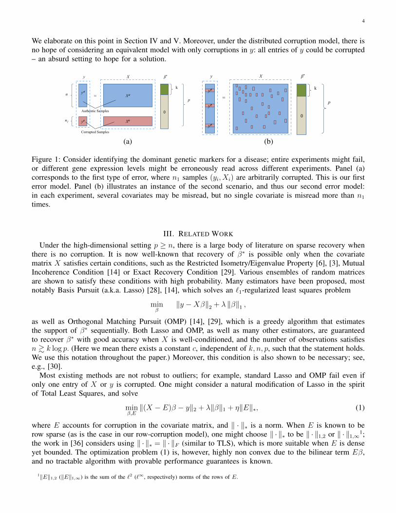
Note that in both models, we impose no assumption whatsoever on the corrupted pairs. They mightbe unbounded, non-stochastic, and even dependent on the authentic samples. They are unconstrainedother than in their cardinality – the number of rows or coefficients corrupted. We illustrate both of thesecorruption models pictorially in Figure 1.

Goal: Given these observations (xi, yi), the goal is to obtain a reliable estimate β of β∗ with correctsupport and bounded error

∥∥∥β − β∗∥∥∥2. A fundamental question, therefore, is to understand in each given

model, given p, n, and k, how many outliers (n1) an estimator can handle.Remark 3. This is a strong notion of robustness. In particular, requiring support recovery is a morestringent requirement than requiring, for example, bounded distance to the true solution, or bounded lossdegradation. It is also worth noting that robustness here is a completely different notion than robustnessin the sense of Robust Optimization (e.g., [2]). There, we seek a solution that minimizes the error weincur when an adversary perturbs our loss function. In contrast, here, here is a true generative model thatobeys the structural assumptions of the problem (namely, sparsity of β∗), but an adversary corrupts thedata that ordinarily provide us with the true input-output behavior of that model.

We emphasize that our setting is fundamentally different from those that only allow corruptions in y,and robust sparse regression techniques that only consider corruption in y are bound to fail in our setting.

4

We elaborate on this point in Section IV and V. Moreover, under the distributed corruption model, there isno hope of considering an equivalent model with only corruptions in y: all entries of y could be corrupted– an absurd setting to hope for a solution.

XO

k

y X β*

yA

=

0

yO

p XA n

n1

Authentic Samples

Corrupted Samples

p

k

y X β*

=

0

yO

yO

yO

(a) (b)

Figure 1: Consider identifying the dominant genetic markers for a disease; entire experiments might fail,or different gene expression levels might be erroneously read across different experiments. Panel (a)corresponds to the first type of error, where n1 samples (yi, Xi) are arbitrarily corrupted. This is our firsterror model. Panel (b) illustrates an instance of the second scenario, and thus our second error model:in each experiment, several covariates may be misread, but no single covariate is misread more than n1

times.

III. RELATED WORK

Under the high-dimensional setting p ≥ n, there is a large body of literature on sparse recovery whenthere is no corruption. It is now well-known that recovery of β∗ is possible only when the covariatematrix X satisfies certain conditions, such as the Restricted Isometry/Eigenvalue Property [6], [3], MutualIncoherence Condition [14] or Exact Recovery Condition [29]. Various ensembles of random matricesare shown to satisfy these conditions with high probability. Many estimators have been proposed, mostnotably Basis Pursuit (a.k.a. Lasso) [28], [14], which solves an `1-regularized least squares problem

minβ

‖y −Xβ‖2 + λ ‖β‖1 ,

as well as Orthogonal Matching Pursuit (OMP) [14], [29], which is a greedy algorithm that estimatesthe support of β∗ sequentially. Both Lasso and OMP, as well as many other estimators, are guaranteedto recover β∗ with good accuracy when X is well-conditioned, and the number of observations satisfiesn & k log p. (Here we mean there exists a constant c, independent of k, n, p, such that the statement holds.We use this notation throughout the paper.) Moreover, this condition is also shown to be necessary; see,e.g., [30].

Most existing methods are not robust to outliers; for example, standard Lasso and OMP fail even ifonly one entry of X or y is corrupted. One might consider a natural modification of Lasso in the spiritof Total Least Squares, and solve

minβ,E‖(X − E)β − y‖2 + λ‖β‖1 + η‖E‖∗, (1)

where E accounts for corruption in the covariate matrix, and ‖ · ‖∗ is a norm. When E is known to berow sparse (as is the case in our row-corruption model), one might choose ‖ · ‖∗ to be ‖ · ‖1,2 or ‖ · ‖1,∞

1;the work in [36] considers using ‖ · ‖∗ = ‖ · ‖F (similar to TLS), which is more suitable when E is denseyet bounded. The optimization problem (1) is, however, highly non convex due to the bilinear term Eβ,and no tractable algorithm with provable performance guarantees is known.

1‖E‖1,2 (‖E‖1,∞) is the sum of the `2 (`∞, respectively) norms of the rows of E.

5

Another modification of Lasso accounts for the corruption in the response via an additional variable z[20], [25], [32], [22]:

minβ,z‖Xβ − y − z‖2 + λ ‖β‖1 + γ ‖z‖1 . (2)

We call this approach Justice Pursuit (JP) after [20]. Unlike the previous approach, the problem (2) isconvex. In fact, it is the natural convexification of the brute force algorithm:

minβ,z

‖Xβ − y − z‖2 (3)

s.t. : ‖β‖0 ≤ k

‖z‖0 ≤ n1,

where ‖u‖0 denotes the number of nonzero entries in u. It is easy to see (and well known) that the so-calledJustice Pursuit relaxation (2) is equivalent to minimizing the Huber loss function plus the `1 regularizer,with an explicit relation between γ and the parameter of the Huber loss function [15]. Formulation (2)has excellent recovery guarantees when only the response variable is corrupted, delivering exact recoveryunder a constant fraction of outliers. However, we show in the next section that a broad class of convexoptimization-based approaches, with (2) as a special case, fail when the covariate X is also corrupted.In the subsequent section, we show that even the original brute force formulation is problematic: whileit can recover from some number n1 of corrupted rows, that number is order-wise worse than what thealgorithm we give can guarantee.

We also note that neither the brute force algorithm above, nor its relaxation, JP, are appropriate for oursecond model for corruption. Indeed, in this setting, modeling via JP would require handling the settingwhere every single entry of the output variable, y, is corrupted, something which certainly cannot be done.

For standard linear regression problems in the classical scaling n p, various robust estimators havebeen proposed, including M -, R-, and S-estimators [18], [24], as well as those based on `1-minimization[19]. Many of these estimators lead to non-convex optimization problems, and even for those that areconvex, it is unclear how they can be used in the high-dimensional scaling with sparse β∗. Anotherdifficulty in applying classical robust methods to our problems arises from the fact that the covariates,xi, also lie in a high-dimensional space, and thus defeat many outlier detection/rejection techniques thatmight otherwise work well in low-dimensions. Again, for our second model of corruption, outlier detectionseems even more hopeless.

IV. FAILURE OF THE CONVEX OPTIMIZATION APPROACH

We consider a broad class of convex optimization-based approaches of the following form:

minβ

f(y −Xβ) (4)

s.t. h(β) ≤ R.

Here R is a radius parameter that can be tuned. Both f(·) and h(·) are convex functions, which can beinterpreted as a loss function (of the residual) and a regularizer (of β), respectively. For example, onemay take f(v) = minz ‖v − z‖2 + γ‖z‖1 and h(β) = ‖β‖1, which recovers the Justice Pursuit (2) byLagrangian duality; note that this f(v) is convex because

‖αv1 + (1− α)v2 − z‖2 + γ‖z‖1 ≤ α(‖v1 − z‖2 + γ‖z‖1) + (1− α)(‖v1 − z‖2 + γ‖z‖1),

by sub-additivity of norms. The function f(·) can also be any other robust convex loss function includingthe Huber loss function.

We assume that f(·) and h(·) obey a very mild condition, which is satisfied by any non-trivial lossfunction and regularizer that we know of. In the sequel we use [z1; z2] to denote the concatenation of twocolumn vectors z1 and z2.

6

Definition 4 (Standard Convex Optimization (SCO) Condition). We say f(·) and h(·) satisfy the SCOCondition if limα→∞ f(αv) =∞ for all v 6= 0, f([v1; v2]) ≥ f([0; v2]) for all v1, v2, and h(·) is invariantunder permutation of coordinates.

We also assume R ≥ h(β∗) because otherwise the formulation is not consistent even when there areno outliers. The following theorem shows that under this assumption, the convex optimization approachfails when both X and y are corrupted. We only show this for our first corruption model, since it is aspecial case of the second distributed model. As illustrated in Figure 1, let A and O be the (unknown)sets of indices corresponding to authentic and corrupted observations, respectively, and XA and XO bethe authentic and corrupted rows of the covariate matrix X = [x1, . . . , xn+n1 ]

>. The vectors yA and yO

are defined similarly. Also let Λ∗ be the support of β∗. With this notation, we have the following.

Theorem 5. Suppose f and h satisfy the SCO Condition. When n1 ≥ 1 and k ≥ 1, the adversary cancorrupt X and y in such a way that for all R with R ≥ h(β∗) the optimal solution does not have thecorrect support.

Proof: Recall that y = [yA; yO] and X = [XA;XO] with yA = XAβ∗+ e, and Λ∗ is the true support.The adversary fixes some set Λ disjoint from the true support Λ∗ with |Λ| = |Λ∗|. It then chooses β andyO such that βΛ = β∗Λ∗ βΛc = 0, and yO = XOβ with XO to be determined later. By assumption wehave h(β) = h(β∗) ≤ R, so β is feasible. Its objective value is f(y −Xβ) = f([yA −XA

Λβ∗Λ∗ ; 0]) ≤ C

for some finite constant C. The adversary further chooses XO such that XOΛ∗ = 0 and XOΛ is large. Anyβ supported on Λ∗ has objective value

f(y −Xβ) = f([yA −XAβ;XO(β − β)]) = f([yA −XAβ;XOΛ β∗Λ∗ ]) ≥ f([0;XOΛ β

∗Λ∗ ]),

which can be made bigger than C under the SCO Condition. Therefore, any solution β with the correctsupport Λ∗ has a higher objective value than β, and thus is not the optimal solution.

Our proof proceeds by using a simple corruption strategy. Certainly, there are natural approaches to dealwith this specific example, e.g., removing entries of X with large values. But discarding such large-valueentries is not enough, as there may exist more sophisticated corruption schemes where simple magnitude-based clipping is ineffective. We illustrate this with a concrete example in the simulation section, whereJustice Pursuit along with large-value-trimming fails to recover the correct support. Indeed, this exampleserves merely to illustrate more generally the inadequacy of a purely convex-optimization-based approach.

More importantly, while the idea of considering an unbounded outlier is not new and has been usedin classical Robust Statistics and more recently in [35], the above theorem highlights the sharp contrastbetween the success of convex optimization (e.g., JP) under corruption in only y, and its complete failurewhen both X and y are corrupted. Corruptions in X not only break the linear relationship between yand X , but also destroy properties of X necessary for existing sparse regression approaches. In the highdimensional setting where support recovery is concerned, there is a fundamental difference between thehardness of the two corruption models.

V. THE NATURAL BRUTE FORCE ALGORITHM

The brute force algorithm (3) can be restated as follows: it looks at all possible n × k submatricesof X and picks the one that gives the smallest regression error w.r.t. the corresponding subvector of y.Formally, let XSΛ denote the submatrix of X corresponding to row indices S and column indices Λ, andlet yS denote the subvector of y corresponding to indices S. The algorithm solves

minθ∈Rk,S,Λ

∥∥yS −XSΛθ∥∥2(5)

s.t. |S| = n,

|Λ| = k.

7

Suppose the optimal solution is S, Λ, θ. Then, the algorithm outputs β with βΛ = θ and βΛc = 0. Notethat this algorithm has exponential complexity in n and k, and Sc can be considered as an operationaldefinition of outliers. We show that even this algorithm has poor performance and cannot handle large n1.

To this end, we consider the simple Gaussian design model, where the entries of XA and e areindependent zero-mean Gaussian random variables with variance 1

nand σe

n, respectively. The 1

nfactor

is simply for normalization and no generality is lost. We consider the setting where σ2e = k and

β∗Λ∗ = [1, . . . , 1]>. If n1 = 0, existing methods (e.g., Lasso and standard OMP), and the brute forcealgorithm as well, can recover the support of β∗ with high probability provided n & k log p. Here andhenceforth, by with high probability (w.h.p.) we mean with probability at least 1 − p−2. However, whenthere are outliers, we have the following negative result.

Theorem 6. Under the above setting, if n & k3 log p and n1 & 3nk+1

, then the adversary can corrupt Xand y in such a way that the brute force algorithm does not output the correct support Λ∗.

The proof is given in Section IX. We believe the condition n & k3 log p is an artifact of our proof andis not necessary. This theorem shows that the brute force algorithm can only handle O

(nk

)outliers. In

the next section, we propose a simple, tractable algorithm that outperforms this brute force algorithm andcan handle O

(n√k

)outliers.

VI. PROPOSED APPROACH: ROBUST MATCHING PURSUIT

The discussion in the last two sections demonstrates that standard techniques for high-dimensionalstatistics and robust statistics are inadequate to handle our problem. As mentioned in the introduction,we believe the key to obtaining an effective robust estimator for high-dimensional data, is simultaneousstructure identification and outlier rejection. In particular, for the sparse recovery problem where theobservations Zi = (xi, yi) reside in a high-dimensional space, it is crucial to utilize the low-dimensionalstructure of β∗ and perform outlier rejection in the “right” low-dimensional space in which β∗ lies. Inthis section, we propose a candidate algorithm, called Robust Matching Pursuit (RoMP), which is basedon this intuition.

Standard MP estimates the support of β∗ sequentially. At each step, it selects the column of X whichhas the largest (in absolute value) inner product with the current residual r, and adds this column to theset of previously selected columns. The algorithm iterates until some stopping criterion is met. If thesparsity level k of β∗ is known, then one may stop MP after k iterations.

To successfully recover the support of β∗, standard MP relies on the fact that for well-conditionedX , the inner product h(j) = 〈r,Xj〉 is close to βj , and thus a large value of h(j) indicates a nonzeroβj . When outliers are present, MP fails because the h(j)’s may be distorted significantly by maliciouslycorrupted xi’s and yi’s. To protect against outliers, it is crucial to obtain a robust estimate of h(j). Thismotivates our robust version of MP.

The proposed Robust Matching Pursuit algorithm (RoMP) is summarized in Algorithms 1 and 2. Similarto standard MP, it selects the columns of X with highest inner products with the residual. There are twomain differences from standard MP. The key difference is that we compute a robust version of innerproduct by trimming large points. Also, there is no iterative procedure – we take the inner productsbetween all the columns of X and the response vector y and selects the top k ones; this leads to a simpleranalysis.

The key idea behind RoMP is that it effectively reduces a high-dimensional robust regression problemto a much easier low-dimensional (2-D) problem, one that is induced by the sparse structure of β∗. Outlierrejection is performed in this low-dimensional space, and the support of β∗ is estimated along the way.Hence, this procedure fulfils our previous intuition of simultaneous structure identification and outlierrejection.

Our algorithm requires two parameters, n1 and k. We discuss how to choose these parameters after wepresent the performance guarantees in the next section.

8

Algorithm 1 Robust Matching Pursuit (RoMP)Input: X, y, k, n1.For j = 1, . . . , p, compute the trimmed inner product (see Algorithm 2):

h(j) = trimmed-inner-product(y,Xj, n1).

Sort |h(j)| and select the k largest ones.Let Λ be the set of selected indices.Set βj = h(j) for j ∈ Λ and 0 otherwise.Output: β

Algorithm 2 Trimmed Inner ProductInput: a ∈ RN , b ∈ RN , n1

Compute qi = aibi, i = 1, . . . , N .Sort |qi| and select the smallest (N − n1) ones.Let Ω be the set of selected indices.Output: h =

∑i∈Ω pi.

VII. PERFORMANCE GUARANTEES FOR ROMPWe are interested in finding conditions for (p, k, n, n1) under which RoMP is guaranteed to recover β∗

with correct support and small error. We consider the following sub-Gaussian design model. Recall thata random variable Z is sub-Gaussian with parameter σ if E[exp(tZ)] ≤ exp(t2σ2/2) for all real t.

Definition 7 (Sub-Gaussian design). Suppose the entries of XA are i.i.d. zero-mean sub-Gaussian variableswith parameter 1√

nand variance 1

n, and the entries of the additive noise are i.i.d. zero-mean sub-Gaussian

variables with parameter σe√n

and with variance σ2e

n.

Note that this general model covers the case of Gaussian, symmetric Bernoulli, and any other distribu-tions with bounded support.

A. Guarantees for the Distributed Corruption ModelThe following theorem characterizes the performance of RoMP, and shows that it can recover the correct

support even when the number of outliers scales with n. In particular, this shows RoMP can tolerate anO(1/

√k) fraction of distributed outliers. Recall that with high probability means with probability at least

1− p−2.

Theorem 8. Under the Sub-Gaussian design model and the distributed corruption model, the followinghold with high probability.

(1) The output of RoMP satisfies the following `2 error bound:∥∥∥β − β∗∥∥∥2

. ‖β∗‖2

√1 +

σ2e

‖β∗‖22

(√k log p

n+n1

√k log p

n

).

(2) If the nonzero entries of β∗ satisfy |β∗j |2 ≥ (‖β∗‖22/n) log p

(1 + σ2

e/ ‖β∗‖22

), then RoMP correctly

identifies the nonzero entries of β∗ provided

n & k log p ·(1 + σ2

e/ ‖β∗‖22

), and

n1

n. 1/

(√k(1 + σ2

e/ ‖β∗‖22

)log p

).

9

The proof of the theorem is given in Section IX. A few remarks are in order.1) We emphasize that knowledge of the exact number of outliers is not needed – n1 can be any

upper bound of the number of outliers, because by definition the adversary can change n1 entriesin each column arbitrarily, and changing less than n1 of them is of course allowed. The theoremholds even if there are less than n1 outliers. Of course, this would result in sub-optimal bounds inthe estimation due to over-conservativeness. In practice, cross-validation could be quite useful here.

2) We wish to note that essentially all robust statistical procedures we are aware of have the samecharacter noted above. This is true even for the simplest algorithms for robustly estimating the mean.If an upper bound is known on the fraction of corrupted points, one computes the analogous trimmedmean. Otherwise, one can simply compute the median, and the result will have controlled error (butwill be suboptimal) as long as the number of corrupted points is less than 50% – something which,as in our case, and every case, is always impossible to know simply from the data.

3) In a similar spirit, the requirement of the knowledge of k can also be relaxed. For example, if weuse some k′ > k instead of k, then under the theorem continues to hold in the sense that RoMPidentifies a superset (with size k′) of the support of β∗, and the `2 error bound holds with k replacedby k′. Standard procedures of estimating the sparsity level (e.g. cross-validation) can also be appliedin our setting.

4) Also note that the term σ2e/ ‖β∗‖

22 has a natural interpretation of signal to noise ratio.

B. Guarantee for the Row Corruption ModelIt follows directly from Theorem 8 that RoMP can handle n1/2 corrupted rows under the same condition.

In fact, a slightly stronger results holds: RoMP can handle n1 corrupted rows. This is the content of thefollow theorem, with its proof given in Section IX.

Corollary 9. Under the Sub-Gaussian design model and the row corruption model with at most n1

corrupted rows, the conclusions of Theorem 8 holds.

Therefore, in particular, our algorithm is orderwise stronger than the Brute Force algorithm, in termsof the number of outliers it can tolerate while still correctly identifying the support.

VIII. EXPERIMENTS

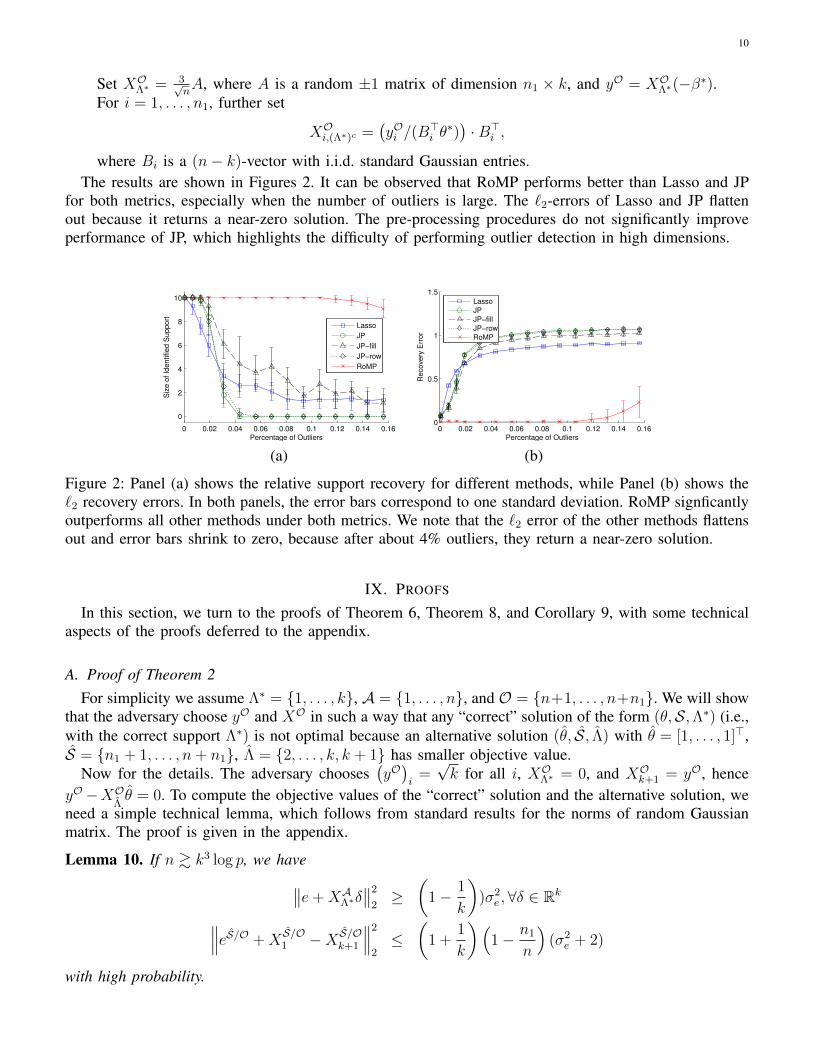
In this section, we report some simulation results for the performance of RoMP (Algorithm 1) onsynthetic data. The performance is measured in terms of support recovery (the number of non-zero locationsof β∗ that are correctly identified), and also relative `2-error (‖β − β∗‖2/‖β∗‖2). The authentic data aregenerated under the sub-Gaussian Design model using Gaussian distribution with p = 4000, n = 1600, k =10 and σe = 2, with the non-zero elements of β∗ being randomly assigned to ±1.

For comparison, we also apply standard Lasso and JP [20], [22] to the same data. For these algorithms,we search for the values of the tradeoff parameters λ, γ that yield the smallest `2-errors, and then estimatethe support using the location of the largest k entries of β. It is also interesting to ask whether a simplemodification of JP would perform well. While not analyzed in any of the papers that discuss JP, weconsider JP with two different pre-processing procedures, both of which aim to detect and correct thecorrupted entries in X directly. The first one, dubbed JP-fill, finds the set E of the largest n1

nportion of

the entries of X , and then scales them to have unit magnitude. The second one, dubbed JP-row, discardsthe n1 rows of X that contain the most entries in E.

The corrupted rows (XO, yO) are generated by the following procedure:Let

θ∗ = arg minθ∈Rp−k:‖θ‖1≤‖β∗‖1

‖yA −XA(Λ∗)>θ‖2.

10

Set XOΛ∗ = 3√nA, where A is a random ±1 matrix of dimension n1 × k, and yO = XOΛ∗(−β∗).

For i = 1, . . . , n1, further set

XOi,(Λ∗)c =(yOi /(B

>i θ∗))·B>i ,

where Bi is a (n− k)-vector with i.i.d. standard Gaussian entries.The results are shown in Figures 2. It can be observed that RoMP performs better than Lasso and JP

for both metrics, especially when the number of outliers is large. The `2-errors of Lasso and JP flattenout because it returns a near-zero solution. The pre-processing procedures do not significantly improveperformance of JP, which highlights the difficulty of performing outlier detection in high dimensions.

0 0.02 0.04 0.06 0.08 0.1 0.12 0.14 0.16

0

2

4

6

8

10

Percentage of Outliers

Siz

e o

f Id

en

tified S

upp

ort

Lasso

JP

JP−fill

JP−row

RoMP

0 0.02 0.04 0.06 0.08 0.1 0.12 0.14 0.160

0.5

1

1.5

Percentage of Outliers

Re

covery

Err

or

Lasso

JP

JP−fill

JP−row

RoMP

(a) (b)

Figure 2: Panel (a) shows the relative support recovery for different methods, while Panel (b) shows the`2 recovery errors. In both panels, the error bars correspond to one standard deviation. RoMP signficantlyoutperforms all other methods under both metrics. We note that the `2 error of the other methods flattensout and error bars shrink to zero, because after about 4% outliers, they return a near-zero solution.

IX. PROOFS

In this section, we turn to the proofs of Theorem 6, Theorem 8, and Corollary 9, with some technicalaspects of the proofs deferred to the appendix.

A. Proof of Theorem 2For simplicity we assume Λ∗ = 1, . . . , k, A = 1, . . . , n, and O = n+1, . . . , n+n1. We will show

that the adversary choose yO and XO in such a way that any “correct” solution of the form (θ,S,Λ∗) (i.e.,with the correct support Λ∗) is not optimal because an alternative solution (θ, S, Λ) with θ = [1, . . . , 1]>,S = n1 + 1, . . . , n+ n1, Λ = 2, . . . , k, k + 1 has smaller objective value.

Now for the details. The adversary chooses(yO)i

=√k for all i, XOΛ∗ = 0, and XOk+1 = yO, hence

yO−XOΛθ = 0. To compute the objective values of the “correct” solution and the alternative solution, we

need a simple technical lemma, which follows from standard results for the norms of random Gaussianmatrix. The proof is given in the appendix.

Lemma 10. If n & k3 log p, we have∥∥e+XAΛ∗δ∥∥2

2≥

(1− 1

k

))σ2

e ,∀δ ∈ Rk

∥∥∥eS/O +XS/O1 −X S/Ok+1

∥∥∥2

2≤

(1 +

1

k

)(1− n1

n

)(σ2

e + 2)

with high probability.

11

Using the above lemma, we can upper-bound the objective value of the alternative solution:∥∥∥yS −X SΛ θ∥∥∥2

2=

∥∥∥yO −XOΛ θ∥∥∥2

2+∥∥∥yS/O −X S/O

Λθ∥∥∥2

2

= 0 +∥∥∥yS/O −X S/OΛ∗ β∗Λ∗ +X

S/O1 −X S/Ok+1

∥∥∥2

2

2

=∥∥∥eS/O +X

S/O1 −X S/Ok+1

∥∥∥2

2

≤(

1 +1

k

)(1− n1

n

)(σ2

e + 2). (6)

To lower-bound the objective value of solutions of the form (θ,S,Λ∗), we distinguish two cases. IfS ∩ O 6= φ, then the objective value is∥∥yS −XSΛ∗θ∥∥2

2≥

∥∥yS∩O −XS∩OΛ∗ θ∥∥2

2

=∥∥yS∩O∥∥2

2

≥ k (7)

If S ∩ O = φ, we have S = A and thus∥∥yS −XSΛ∗θ∥∥2

2=

∥∥yA −XAΛ∗θ∥∥2

2∥∥XAΛ∗β∗Λ∗ + e−XAΛ∗θ∥∥2

2

=∥∥e+XAΛ∗(β

∗ − θ)∥∥2

2

≥(

1− 1

k

)σ2e (8)

where we use the lemma. When n1 >3nk+1

and σ2e = k, we have min

k,(1− 1

k

)σ2e

>(1 + 1

k

) (1− n1

n

)(σ2

e+2). Combining (6) (7) and (8) concludes the proof.

B. Proof of Theorem 3We prove Theorem 3 in this section. We need two technical lemmas. The first lemma bounds the

maximum of independent sub-Gaussian random variables. The proof follows from the definition of sub-Gaussianity and Chernoff bound, and is given in the appendix.

Lemma 11. Suppose Z1, . . . , Zm are m independent sub-Gaussian random variables with parameter σ.Then we have maxi=1,...,m |Zi| ≤ 4σ

√logm+ log p. with high probability.

The second lemma is a standard concentration result for the sum of squares of independent sub-Gaussianrandom variables. It follows directly from Eq. (72) in [23].

Lemma 12. Let Y1, . . . , Yn be n i.i.d. zero-mean sub-Gaussian random variables with parameter 1√n

andvariance at most 1

n. Then we have

|n∑i=1

Y 2i − 1| ≤ c1

√log p

n

with high probability for some absolute constant c1. Moreover, if Z1, . . . , Zn are also i.i.d. zero-mean sub-Gaussian random variables with parameter 1√

nand variance at most 1

n, and independent of Y1, . . . , Yn,

then

|n∑i=1

YiZi| ≤ c2

√log p

n

with high probability for some absolute constant c2.

12

Remark 13. When the above inequality holds, we write∑n

i=1 Y2i ≈ 1±

√log pn

and∑n

i=1 YiZi ≈ ±√

log pn

.w.h.p.

Now consider the trimmed inner product h(j) between the jth column of X and y. Let Aj is the set ofindex i such that Xij and yi are both not corrupted. By assumption |Aj| ≥ n. By putting |Aj| − n cleanindices in Acj , we may assume |Aj| = n without loss of generality. By prescription of Algorithm 2, wecan write h(j) as

h(j) =∑i∈Aj

Xijyi −∑

i∈trimmedinliers

Xijyi +∑

i∈remainingoutliers

Xijyi.

We estimate each term in the above sum.1) Observe that∑

i∈Aj

Xijyi =∑i∈Aj

Xij

(p∑

k=1

Xikβ∗k + e

)=∑i∈Aj

X2ijβ∗j +

∑i∈Aj

Xij

(∑k 6=j

Xikβ∗k + e

).

(a) Because the points in Aj obeys the Sub-Gaussian model, Lemma 12 gives∑

i∈AjX2ijβ∗j ≈

β∗j

(1±

√1n

log p)

w.h.p.

(b) On the other hand, because Xik and Xij are independent when k 6= j, and Zi ,∑

k 6=j Xikβ∗k +e

are i.i.d. sub-Gaussian with parameter and standard deviation at most√(‖β∗‖2

2 + σ2e

)/n, we apply

Lemma 12 to obtain∑

i∈AjXijZi ≈ ± 1√

n

√(‖β∗‖2

2 + σ2e

)log p w.h.p.

2) Again due to independence and sub-Gaussianity of points in Aj , Lemma 11 gives maxi∈Aj|Xij| .√

(log p)/n w.h.p. and maxi∈Aj|yi| .

√(log p/n)

(‖β∗‖2

2 + σ2e

)w.h.p. It follows that w.h.p.∣∣∣∣∣∣∣

∑i∈trimmed

inliers

Xijyi

∣∣∣∣∣∣∣ ≤ n1

(maxi∈A|Xij|

)(maxi∈A|yi|)

. n1 ·√

log p

n·√

log p

n

(‖β∗‖2

2 + σ2e

).

3) By prescription of the trimming procedure, either all outliers are trimmed, or the remaining outliersare no larger than the trimmed inliers. It follows from the last equation that w.h.p.∣∣∣∣∣∣∣

∑i∈remaining

outliers

Xijyi

∣∣∣∣∣∣∣ ≤∑

i∈remainingoutliers

|Xijyi| ≤∑

i∈trimmedinliers

|Xijyi| . n1log p

n·√‖β∗‖2

2 + σ2e .

Combining pieces, we have for all j = 1, . . . , p,∣∣h(j)− β∗j∣∣ . ∣∣β∗j ∣∣√ 2

nlog p+

1√n

√(‖β∗‖2

2 + σ2e

)log p+ n1 ·

log p

n

√(‖β∗‖2

2 + σ2e

). (9)

If RoMP correctly picks an index j in the true support Λ∗, then the error in estimating βj is boundedby the expression above. If RoMP picks some incorrect index j not in Λ∗, then the difference betweenthe corresponding βj and the true β∗j′ that should have been picked is still bounded by the expressionabove (up to constant factors). Therefore, we have∥∥∥β − β∗∥∥∥2

2.∑j∈Λ∗

[∣∣β∗j ∣∣√ 2

nlog p+

1√n

√(‖β∗‖2

2 + σ2e

)log p +n1

log p

n

√(‖β∗‖2

2 + σ2e

)]2

.

13

The first part of the theorem then follows after straightforward algebra manipulation. On the other hand,RoMP picks the correct support as long as |h(j)| > |h(j′)| for all j ∈ Λ∗, j′ ∈ (Λ∗)c. In view of Eq.(9),we require

n & maxj

(‖β∗‖2

2

β2j

)· log p ·

(1 + σ2

e/ ‖β∗‖22

)n1

n.

1√maxj

(‖β∗‖22β2j

)·(1 + σ2

e/ ‖β∗‖22

)log p

One verifies that the above inequalities are satisfied under the conditions in the second part of the theorem.

C. Proof of Corollary 1A careful examination of the proof of Theorem 2 in the last section shows that, when there are n1

corrupted rows, the set Aj still has cardinality at least n, and the proof thus holds under the row corruptionmodel.

X. CONCLUSION

Adversarial corruption seems to be significantly more difficult than corruption independent from theoriginal data, and moreover, corruption in X as well as y appears more challenging than corruption only iny. To the best of our knowledge, no prior existing algorithms have provable performance in this setting, orin the more difficult yet setting of distributed corruption. This paper provides the first results for both thesesettings. Our results outperform Justice Pursuit, as well as the exponential time Brute Force algorithm;more generally we show that no convex optimization based approach improve on the results we provide.Generalizing our results to obtain a sequential OMP-like algorithm, and on the other side, understandingconverse results, are important next steps.

REFERENCES

[1] R. Baraniuk, M. Davenport, R. DeVore, and M. Wakin. A simple proof of the restricted isometry property for random matrices.Constructive Approximation, 28(3):253–263, 2008.

[2] D. Bertsimas, D. B. Brown, and C. Caramanis. Theory and applications of robust optimization. SIAM Review, 2011.[3] P.J. Bickel, Y. Ritov, and A.B. Tsybakov. Simultaneous analysis of lasso and dantzig selector. The Annals of Statistics, 37(4):1705–1732,

2009.[4] E. Candes and T. Tao. The dantzig selector: Statistical estimation when p is much larger than n. The Annals of Statistics, 35(6):2313–

2351, 2007.[5] E.J. Candes, X. Li, Y. Ma, and J. Wright. Robust principal component analysis? Arxiv preprint arXiv:0912.3599, 2009.[6] E.J. Candes and T. Tao. Decoding by linear programming. Information Theory, IEEE Transactions on, 51(12):4203–4215, 2005.[7] V. Chandrasekaran, S. Sanghavi, S. Parrilo, and A. Willsky. Rank-sparsity incoherence for matrix decomposition. SIAM Journal on

Optimization, 21(2):572–596, 2011.[8] S.S. Chen, D.L. Donoho, and M.A. Saunders. Atomic decomposition by basis pursuit. SIAM journal on scientific computing, 20(1):33–

61, 1999.[9] Y. Chen and C. Caramanis. Orthogonal matching pursuit with noisy and missing data: Low and high dimensional results. arXiv preprint

arXiv:1206.0823, 2012.[10] Y. Chen and C. Caramanis. Noisy and missing data regression: Distribution-oblivious support recovery. In International Conference

on Machine Learning, 2013.[11] Yudong Chen, Huan Xu, Constantine Caramanis, and Sujay Sanghavi. Robust matrix completion with corrupted columns. Submitted.

Arxiv Preprint arXiv:1102.2254v1, 2011.[12] M.A. Davenport and M.B. Wakin. Analysis of orthogonal matching pursuit using the restricted isometry property. Information Theory,

IEEE Transactions on, 56(9):4395–4401, 2010.[13] D. L. Donoho. Breakdown properties of multivariate location estimators, qualifying paper, Harvard University, 1982.[14] D.L. Donoho, M. Elad, and V.N. Temlyakov. Stable recovery of sparse overcomplete representations in the presence of noise. Information

Theory, IEEE Transactions on, 52(1):6–18, 2006.[15] J.J. Fuchs. An inverse problem approach to robust regression. In Acoustics, Speech, and Signal Processing, 1999. ICASSP’99.

Proceedings., 1999 IEEE International Conference on, volume 4, pages 1809–1812. IEEE, 1999.[16] F.R. Hampel, E.M. Ronchetti, P.J. Rousseeuw, and W.A. Stahel. Robust statistics: the approach based on influence functions, volume

114. Wiley, 1986.

14

[17] M.A. Herman and T. Strohmer. General deviants: An analysis of perturbations in compressed sensing. Selected Topics in SignalProcessing, IEEE Journal of, 4(2):342–349, 2010.

[18] Peter Huber. Robust Statistics. Wiley, New York, 1981.[19] V. Kekatos and G.B. Giannakis. From sparse signals to sparse residuals for robust sensing. Signal Processing, IEEE Transactions on,

59(7):3355–3368, 2011.[20] J.N. Laska, M.A. Davenport, and R.G. Baraniuk. Exact signal recovery from sparsely corrupted measurements through the pursuit of

justice. In Signals, Systems and Computers, 2009 Conference Record of the Forty-Third Asilomar Conference on, pages 1556–1560.IEEE, 2009.

[21] G. Lerman, M. McCoy, J.A. Tropp, and T. Zhang. Robust computation of linear models, or how to find a needle in a haystack. Arxivpreprint arXiv:1202.4044, 2012.

[22] Xiaodong Li. Compressed sensing and matrix completion with constant proportion of corruptions. Arxiv preprint arXiv:1104.1041,2011.

[23] P.L. Loh and M.J. Wainwright. High-dimensional regression with noisy and missing data: Provable guarantees with non-convexity.Annals of Statistics, 40(3):1637–1664, 2012.

[24] R.A. Maronna, R.D. Martin, and V.J. Yohai. Robust statistics. Wiley, 2006.[25] N.H. Nguyen, T. Tran, et al. Exact recoverability from dense corrupted observations via l_1 minimization. Arxiv preprint

arXiv:1102.1227, 2011.[26] M. Rosenbaum and A.B. Tsybakov. Sparse recovery under matrix uncertainty. The Annals of Statistics, 38(5):2620–2651, 2010.[27] M. Rosenbaum and A.B. Tsybakov. Improved matrix uncertainty selector. arXiv preprint arXiv:1112.4413, 2011.[28] R. Tibshirani. Regression shrinkage and selection via the lasso. Journal of the Royal Statistical Society. Series B (Methodological),

pages 267–288, 1996.[29] J.A. Tropp. Greed is good: Algorithmic results for sparse approximation. Information Theory, IEEE Transactions on, 50(10):2231–2242,

2004.[30] M.J. Wainwright. Information-theoretic limits on sparsity recovery in the high-dimensional and noisy setting. Information Theory,

IEEE Transactions on, 55(12):5728–5741, 2009.[31] M.J. Wainwright. Sharp thresholds for high-dimensional and noisy sparsity recovery using-constrained quadratic programming (lasso).

Information Theory, IEEE Transactions on, 55(5):2183–2202, 2009.[32] J. Wright and Y. Ma. Dense error correction via-minimization. Information Theory, IEEE Transactions on, 56(7):3540–3560, 2010.[33] H. Xu, C. Caramanis, and S. Mannor. Outlier-Robust PCA: The High Dimensional Case. IEEE Transactions on Information Theory,

59(1):546–572, 2013.[34] H. Xu, C. Caramanis, and S. Sanghavi. Robust PCA via outlier pursuit. IEEE Transactions on Information Theory, 58(5):3047–3064,

2012.[35] Y. Yu, O. Aslan, and D. Schuurmans. A polynomial-time form of robust regression. In Advances in Neural Information Processing

Systems 25, pages 2492–2500, 2012.[36] H. Zhu, G. Leus, and G.B. Giannakis. Sparsity-cognizant total least-squares for perturbed compressive sampling. Signal Processing,

IEEE Transactions on, 59(5):2002–2016, 2011.

APPENDIX

Let θ′ =[σe|δ>

]>. We can write∥∥e+XAΛ∗δ

∥∥2

2= ‖Z1θ

′‖22 with Z1 ,

[1σee|XAΛ∗

]. Note that Z1 is an

n×(k+1) matrix with i.i.d. N (0, 1n) entries, whose smallest singular value can be bounded using standard

results. For example, using Lemma 5.1 in [1]with Φ(ω) = Z1, N = k + 1, T = 1, . . . , N, δ = 13k

andc0(δ/2) = 1/288k2, we have

‖Z1θ′‖2

2 ≤(

1 +1

3k

)2 ‖θ′‖2

2 ≤(

1 +1

k

)σ2e ,∀δ

with probability at least1− 2e

1288k2

n−(k+1) ln(36k) ≥ 1− 2p−3

provided n ≥ 576(k + 1)3 ln(36p). This proves the first inequality.Let Z = maxi Zi. By definition of sub-Gaussianity, we have

E[etZ/σ

]= E

[maxietZi/σ

]≤

∑i

E[etZi/σ

]≤ met

2/2

= et2/2+logm

15

It follows from Markov Inequality that

P (Z ≥ σt) = P (etZ/σ ≥ et2

)

≤ e−t2E[etZ/σ

]≤ e−t

2+t2/2+logm

= e−12t2+logm.

By symmetry we haveP (min

iZi ≤ −σt) ≤ e−

12t2+logm,

so a union bound gives

P (maxi|Zi| ≥ σt) ≤ P (max

iZi ≥ σt) + P (min

iZi ≤ −σt)

≤ 2e−12t2+logm.

Taking t = 4√

logm+ log p yields the result.