1-s2.0-0043164894065454-main

7/27/2019 1-s2.0-0043164894065454-main

http://slidepdf.com/reader/full/1-s20-0043164894065454-main 1/18

WEARELSEVIER Wear 180 (1995) 17-34

Generalized fractal analysis and its

surfaces

applications to engineering

Suryaprakash Ganti, Bharat Bhush anComputer M icrotri boIqy and Contamination Laboratory, D epartment of Mechanical Engineerin g, The Ohio State University, Columbus,

OH 43210-1107, USA

Received 9 March 1994; accepted 29 September 1994

Abstract

Fractal analysis previously developed for surface characterization is generalized and an intrinsic length unit (Y n this analysis

has been taken aslateral r esoluti on of the measur ing instrument 7).

This generalized analysis allows the surface characterizationin terms of two fractal parameters-fractal dimension D and amplitude coefficient C, which, in theory, are instrument independent

and unique for each surface. A powerful technique is developed for the simula tion of fractal surface profiles. B ased on the

generation of random surfaces of various D and C values, we note that D primarily relates to relative power of the frequency

contents and C to the amplit ude of all frequencies. A numb er of engineering surfaces-p articulate magne tic tapes, thin-film

rigid disks, steel disks, plastic disks and diamon d films, all of varying roughnesses were measured to validate the generalized

fractal analysis. W e have obtained D and C parameters for each engineering surface from the measurements made using two

instrume nts with significantly different resolutions. The variation in C within each surface is attributed to the simplified

assumption of lateral resolution as the intrinsic length unit. We found that for a given surface with varying roughnesses, D

essentially remains constant and to a first order C varies monotonically with variance of surface heights (u’) for a given

instrument. Simulated u shows similar trends to the measured (T for small scan lengths. Coefficient of friction of all surfaces

has reasonable correspondence with C. Based on this study, the fractal parameter C may better represent the variance for

tribological surfaces.

Keywords: Fractal analysis; Engineering surfaces

1. Introduction

The surface roughness plays an important role in

friction and wear of sliding surfaces. Characterization

of rough ness is a necessary step in their s tudy. The

roughness of a surface is made of an infinite number

of frequencies rangin g from atomic scale to scales

comparable to scan length. Many authors [l-3] have

treated surfaces as random processes. Their roughness

characterization theories consider a surface to be a

stationary process (to be described later) and usestatistical parame ters such as variance of surface heig hts,

surface slope and curvature and the rrns of the peak

heights, peak slopes and peak curvatures for surface

characterization and contact mod elling [4]. If a surface

behaves as a stationary process, variance of the surface

heights should be independent of scan length. However

it has been sh own [5] that these surface parameters

are strongly dependent on the scan length and the

measurement technique and hence are not unique for

a surface. Fig. 1 show s variation of variance of surface

height, slope and curvature for a magnetic tape, magnetic

disk and polished steel (AISI 52 100) disk. We note

that variance generally increases with scan length except

at high values. At large scan lengths it drops because

of a change in the measuring instrument. A dip in the

variance of slopes is observed for sma ll scan lengths.

For the case of magn etic tape, this is due to the different

surface characteristics of the particles comp ared with

the surface at a larger scale. For magnetic disk and

steel, we speculate that the morphology of the grainscauses a dip on a smaller scale. The curvature decreases

with scan length in all cases, as expected. We note

that surfaces behave as nonstationary processes with

generally increasing variance for increasing scan length

[6]. Hence the traditional surface characterization the-

ories are based on a few length scales depending on

the scan length and resolution of the instrument unlike

the large number of frequencies that make up the

surface. In order to characterize rough ness at all scales,

a scale-indepen dent parametrization is required.

0043-1648/95/$09.50 0 1995 Elsevier Science S.A. All rights reserved

SSDI 0043-1648(94)06545-4

7/27/2019 1-s2.0-0043164894065454-main


18 S. Gad, B. Bhushan / Wear 180 (1995) 17-34

0 50 100 150 200 250

Scan length, pm

Fig. 1. Variation of surface parameters a, CT’ nd d’ with scan length

for (a) magnetic tape, (b) magnetic disk and (c) lapped steel disk

measured using an atomic force microscope (AFM) and a noncontact

optical profiler (NOP).

A unique property exhibited by some rough surfaces

is that if a surface is repeatedly magn ified, increasing

details of roughness are observed right down to the

nanoscales. Fig. 2 shows the multi-scale nature of a

lapped steel surface at 50 pm and 4000 pm scan lengths.

The profiles at two scan lengths look very similar except

for the vertical sca le (self-affine). Fractal analysis allow s

the mod elling of multi-scale nature of self-affine sur-

faces.

The fractal n ature of a variety of engineering surfaceshas been show n by Majum dar and Bhushan [7] (also

see [S-lo]); m ountain s, co astlines a nd fractured surfaces

by Mandelbrot et al. [11,12] and polymers by Aldissi

[13]. The fractal approach [7] has the ability to char-

acterize rough ness by scale-indepen dent paramete rs and

hence to predict the surface characteristics at all scan

lengths by making measurements at one scan length.

Majum dar and Bhushan [7] developed the fractal theory

based on the modified Weierstrass-Mandelbrot (W-M )

function

Distance, pm

Distance, pm

Fig. 2. An NOP image at 4000 pm scan length and an AFM image

at 50 Km scan length for a lapped steel surface.

m cos(279Q)z(x) = GD-’ x

(2 -D)n1<0<2 y>l

n=n, y(1)

where y” are the discrete frequency mod es, IZ ~ s the

low cut-off frequency of the profile, D is the fractal

dimen sion of the profile and G is a scaling coefficient.

Accordin g to this analysis, the variance (z’(x)) increase s

with the scan length and hence it represents a non-

stationary process [14]. For an isotropic fractal surface,the study of a section p rovides complete information

about the surface as the fractal dimen sion D of the

profile and that of the surface D, are related as D, = D + 1

[11,15] and as the profile a nd surface spectral densities

are related [2]. Based on Majumdar and Bhushan’s

analysis, such a surface can be characterized using the

parameters D and G (Majumd ar and Bhushan or M-B

model). The power spectrum and the structure function

of the modified W-M function (Eq. (1)) follow power

laws and are given by

Gz(D- 1)

P(w) =05_2D (2a)

S(T)=kG*(=-1)74-=’

(2b)

where k = r(m - 3) sin] (20 - 3w21

2-D

The power law behavior of the power spectrum and

structure function im plies that a corresponding nonsta-

tionary process has stationary increments which is essential

for defining surface roughness (for further discuss ions,

see later in this paper). The p lots of P(w) as a function

of w and S (r) as a function of r in Eq. (2) are stra ight

7/27/2019 1-s2.0-0043164894065454-main


S. Gad, B. Bhushan / Wear 180 (1995) 17-34 19

lines in the log-log plot. Majumdar and Bhushan have

shown that the power function and the structure function

of a variety of surfaces follow a power law behavior

[7,16-201. A lateral shift in the structure and power

function plots wa s observed for mos t of the surfaces

with a change in the lateral resolution of the instrumen t

but their slope remained constant. This shows that D

is unique and is independent of the scan length; however,

G is not unique. The lateral shift cannot be explained

by W-M function if G is considered to be scale in-

dependent. Hence a more basic understanding of these

nonstationary processes w ith power law behavior for

their structure and power functions is essential.

Mean = p = (x(t))

Variance = a2 = (x’(t)) - p*

Autocovariance function =B= (T) = (x ( t) x ( t + T) )

where L is the sample length.

Power spectral density function

iI1 I2

=qo>=;;_ x(t)eiol dt

In this paper we develop a generalized fractal analy sis

for a fractional Brow nian motion (fBm), an example

of a nonstationary process with stationary incremen ts

(NSPSI) which has been shown to be fractal by Man-

delbrot [ll] and all fractal analy ses for characterization

of surface roughness (including M -B model) assume

NSPSI. The new structure function exhibits the powerlaw behavior which is similar to that in the W-M

function except that the new function includes a meas-

uring length un it. The lateral resolu tion of the instru-

ment, a non-infinitesimal quantity, is used as a measuring

length unit (similar to the length unit in the calculation

of fractal dim ension of surfaces using the length-nu mber

relation proposed by Man delbrot) in the analysis . Scale-

indepen dent param eters, that characterize a surface

better then variance and other standard surface pa-

rameters, are obtained . The method developed for the

generation of fractal profiles is explained and an explicit

form for the variance in terms of the new parametrization

given. This is followed by measurements on varioussurfaces to validate our theory a nd to provide a char-

acterization based on a set of scale-indepen dent pa-

rameters. Correlation between variance and coefficient

of friction with measu red fractal parameters for various

surfaces is sought.

Structure function = S(T) = ([x(t) -x(t + 7)]‘) (7)

Relationship between the power and structure func-

tions:

m

S(r) = s (1- eio’)P(w) do

-m

2.1.2. Random processes

Since a surface is treated as a random process, the

types of processes that are relevant to this paper are

defined here.

2. Generalized fractal analysis

A process x(t) is stationary in the strict sense if the

distribution of x(t) is independent of t, and if all the

moments and joint moments are invariant w ith respect

to a translation in t [23 ] . A Bernoulli random process

of an unendin g sequence of flips of a coin is a stationary

process in the strict sense. If prob(X ,= head in the

nth flip) =p, then th e variance of this process isp(1 -p),

which is a constant. This means that the probabilitydistribution function should not depend on the sample

length (preceding or following events). This is not true

for surfaces as the variance of the surface heigh ts is

scale dependent. B=( t ) represents the autocovariance

function for a samp le leng th L and hence has a de-

pendence on L in general. If the autocovariance function

is independent of L , it is represented by B(T) . For a

process x(t) that has a second order moment with a

constant mean value, if

2.1. Basic def in i t ions for random sur jkes B=(T) = (x ( t) x ( t+ 7)) “B(T)

T he height at any point on the surface can beconsidered as a random variable [2]. A random process

consists of an infinite family of random variables. Hence

the roughness can be considered as a random process

[2,4]. In this section, the common statistical param eters

and various types of random processes used in the

fractal analysis are defined.

2.1.1. Statistical parameters

For a random process x(t), the following statistical

parame ters are defined h ere and are used later [21,22,5].

i.e. it is just a function of r and not a function of L ,

then the process is stationary in the weak sense. Considerfor example x( t) =A4( t) where A is a random variable

with (A) =0 and (A ’) =constant. If 4( t)= e’ & , then

B(T) = (A2)eiwr and hence is a stationary process in the

weak sense. If the first and second order moments are

functions of t, then the process x( t) is non-stationary.

Binomial counting process with probability distribution

p(X , = k ) = (“k )pk ( 1 -p)” - k is an example of a nonsta-

tionary process as variance =np( 1 p) and hence de-

pends on the number of trials n. This process includes

all the possib ilities of dependen ce of the neighboring

(3)

(4)

(5 )

(6)

(8)

7/27/2019 1-s2.0-0043164894065454-main


20 S. Ganti, B. Bhushan / Wear 180 (1995) 17-34

events. Surface ro ughn ess being a function of scan

length is an example of nonstationary process.

Cons ider a non-stationary random process x(t). Let

Ap==x (t +k) -x(t). Ad is termed as an increment. If

the increments, Akx, have a distribution which depends

only on k , and not on the sample length or the number

of trials, then the nonstationary process is said to have

stationary increments (in the weak sense). For examplethe Wiener process with the probability distribution

v41

has a variance = C t and hence is nonstationary but the

variance of the incremen ts is proportional to It-to] and

hence has stationary incremen ts. The nonstationary

processes with stationary increments (NSPSI) possess

the property of self-affinity as will be discussed later.

2.2. Select i on o f s t r uc t u r e func t i on in thecha rac ter i za t i on o f su$aces

A Gaussian random process can be defined completely

by its mean and the autocovariance function. In general,

the tilt from a surface is removed and hence its mean

is zero. It is to be noted that the structure function

and the autocovariance function are related by [22]

S(r) = 2]&(O) -&x41 (10)

It is clear tha t S(r) is bound ed by

S(T) <4&.(O)

It can be seen from E q. (10) that, if we know &(T),

we can determine S(r) bu t the converse is not necessarily

true. However, if

(x(t)> = 0

lim BL( 7) = 07-m

then S(r) and B(r) are interchange able and

For almo st all engineering surfaces observed , the

autocovariance function dies dow n for sufficiently large7. Hence for a particular scan length L , as T - + L ,

S(T)- >2J3,(0)=22 where c2 is the variance at that

scan length. This represents the flat portion observed

in the structure functions for almo st all the surfaces.

It has been observed that the structure function can

be calculated from a set of height data w ith greater

accuracy than the autocovariance and the power spectral

density function s [22]. The power function is calculated

by transformin g the discrete heights into the frequency

domain w hich results in an approximation. Structure

function is calculated directly from the height infor-

mation and results in a better approximation. Since

the structure function is always positive, cancellation

errors are also avoided un like the autocovariance func-

tion. We use the structure function in the present

analysis because of its uniqueness and high accuracy.

2.3. Genera l exp ress ion fo r s t r u c t u r e j i u zc t i on o f

n on s t a t i o n a r y p r o ces ses w i t h st a t i o n a l y i n c r emen t s

(NSPS I )

Engin eering surfaces have multi-scale na ture, in-

creasing variance with scan length, power law behavior

for their structure and power function s and have the

property of self-affinity [7]. All these properties can

be found in an NSPSI.

An NSPSI is nonstationary and has increasing variance

[25]. It is non-differentiable everywhere in its dom ain

and hence satisfies the criterion that roughnes s exists

at all scales. For an NSPSI, it has been shown that[22,261

S(7)=C7m O < m < 2 (11)

and m is related to the fractal dimension, D by the

relation [28]

2D=4 -m (12)

For a real, non-differentiable process

S(r) = j+(I - cos w ,) P (o ) du (13)0

Hence the power fun ction for an NSP SI follows

P ( w ) = - &

where

(14)

1cl= m c

s(l-cosx)Km-l dK

0

=r (m + 1) sin(m/2) c

2rr

Hence b oth the structure and power functions follow

power laws.

The processes w hich have the structure function given

by Eq. (1 1) have a special form. Th eir form is invariant

under a group of similarity transforma tions

t * h t x+ y ( h ) x (15a)

S(T) = y* S(hT) (15b)

y = h - “ “ ’ (15c)

7/27/2019 1-s2.0-0043164894065454-main


S. Ganti, B. Bhushan I Wear 180 (1995) 17-34

This property. i s called self-affinity as the scaling is

different in both the horizontal and vertical directions.

It has been sho wn that stationary processes do not

possess this property. Hence a surface can be assumed

to be a NSP SI if it has the properties mention ed earlier.

The W -M function [16] satisfies all the above conditions

and can be treated as NSPSI. However as we have

stated earlier, W-M function does not take into account

the lateral reso lution of the instrum ent and hence the

lateral shift in the structure functions at different scan

lengths.

NSPSI as described earlier does not have an intrinsic

length unit. To overcome the said difficulties a nd to

develop a general expression, the Gaussian process of

Brownian motion and fractional Brownian motion are

considered. Brownian motion (Bm) is shown to be

fractal and the concept of fractional Brow nian motion

(fBm) was introduced by Mandelbrot [ll] as a gen-

eralization of Bm. The well-known Wiener process

represents Bm and is an NSPSI with probability dis-tribution given by

dx@>4to)l =&G&qxp[x(t) -x(~o)12- 4Clt - toI I (16)

The incremen ts x(t)-x(t,) are Gau ssian in nature

and are indepen dent of each other. Wiener process is

a starting point for the derivation of fBm. fBm is a

NSPSI w hich has a characteristic length unit. The

incremen ts of this process are generalized to give fBm

by the modification [26,27]

x(t) -x(tJ _ qt - to]Z-D (17)

where 5 is a Gaussian random value. D= 1.5 gives the

stand ard Bm. Hence for the fBm, the normalized vari-

able for the incremen ts can be written as

40 --Go)y=mG[ t--tolla]2-D

(18)

where (Y s a non-infinitesimal quantity. It is similar to

a meas uring length u nit in the calculation of fractal

dimen sion (similarity dimen sion) for a profile using the

traditional methods [11,25].

Mean = (x(t) -x(t + 7)) = 0

Varianc e of the increments is the structure function

of the fBm and can be obtained as

S(7)=a”(t--to)=C~~-374-- (19)

where 7 is the size of the increment. We have taken

(r as the reso lution of the instrum ent, q. In fact (Y an

be a function of the resolution of the instrument, grain

size and other intrinsic length units of the specimen.

Hence the structure and power functions with lateral

resolution taken into account are given by (Ganti and

Bhushan or G-B m odel)

21

(20)

(21)

where

1

cl= mc

s(1-cosxzy-(~-+lX

0

=r(5-2D)sin[ 42-D)] c

2r r

It is clear that D and C characterize these surfaces

completely and hence provide a machine-independent

parametrization. D relates to the relative power of the

frequency contents and C relates to the amp litude of

all frequencies. The difference between this structure

function and the one obtained from modified W -M

function is that it takes into account the measuringlength unit (in this case the lateral resolution of the

measuring instrument) and hence the lateral shift ob-

served in the structure functions of experimen tal data.

At D = 1.5, there is no effect of n and hence no shift

in the structure function will be observed. At this

condition, structure function is same as that for W-M

function [29].

3. Fractal simulation

To provide a qualitative and quantitative picture ofthe surface profiles at all scan lengths, a simple technique

is developed here to simulate an ideal surface of a

particular D and C and for a given scan length. The

simulation starts from an ideal power spectrum of a

surface. For an ideal surface of fractal parameters D

and C, the power spectrum is a ‘straight line in the

log-log plot. This forms the starting point for the

generation of complex frequencies. A mach ine-built

random number generator is used to generate the

amp litudes of the frequency comp onents.

Let the profile be discretized at N points. To simplify

the calculations and to use the fast Fourier transform

(FIT) we choose N to be a power of 2. Let h i be theheight at the jth node and H k , its Fourier pair. So

according to NSPSI,

Power at frequency f k k j o = c2T :oF_2D (22)

where C, is C~w -3 an d f . is the fundamental

frequency = l/L, L being the length of the sample. By

definition

7/27/2019 1-s2.0-0043164894065454-main


22 S. Ganti, B. Bhushan I Wear 180 (1995) 17-34

IHkl”= CIKw377%)‘-w

We choose initially

(23b)

Re H k = random sign * random[ \/r.(&J

0,

Im H k = random sign *

t l kE 0 , ;

[ )

Consider

H k ’ = $ {H k + H & } (24)

where H& ,represents the complex conjugate of HN - - * .

The power spectrum I H k ’ 1 2 appears as a horizontal

line as shown in Fig. 3.

This method makes sure that the heights we get are

real with no imaginary parts. Now we make Hkr obey

the pow er law by the followin g m odification:

W)

I ’ I

I : II

I

1 ’I

II

9 a ma-@,

Frequency

Fig. 3. Power spectral density function for a simulated fractal profile

Hk’= ( k +1 - i ,2 )f o ] 5 -W H k ’‘ i i <k,N-1 (25b)

Now the power spectrum appears as V-shaped as

shown in Fig. 3. FFT is used to convert these complex

frequencies to real heights . The pseudo rand om g en-eration of the sign for the real and imaginary parts

creates a random phase for the height profile.

Based on the fractal an alysis, it can be seen from

Eq. (21) that the power dies down as w-(5--20). There-

fore, D affects the rate at which the power dies down

and hence dictates the influence of higher frequen cies.

Relative power of high frequencies increases at higher

values of D . C affects the amplitud es of all frequencies

and hence influences the roughness at global level (all

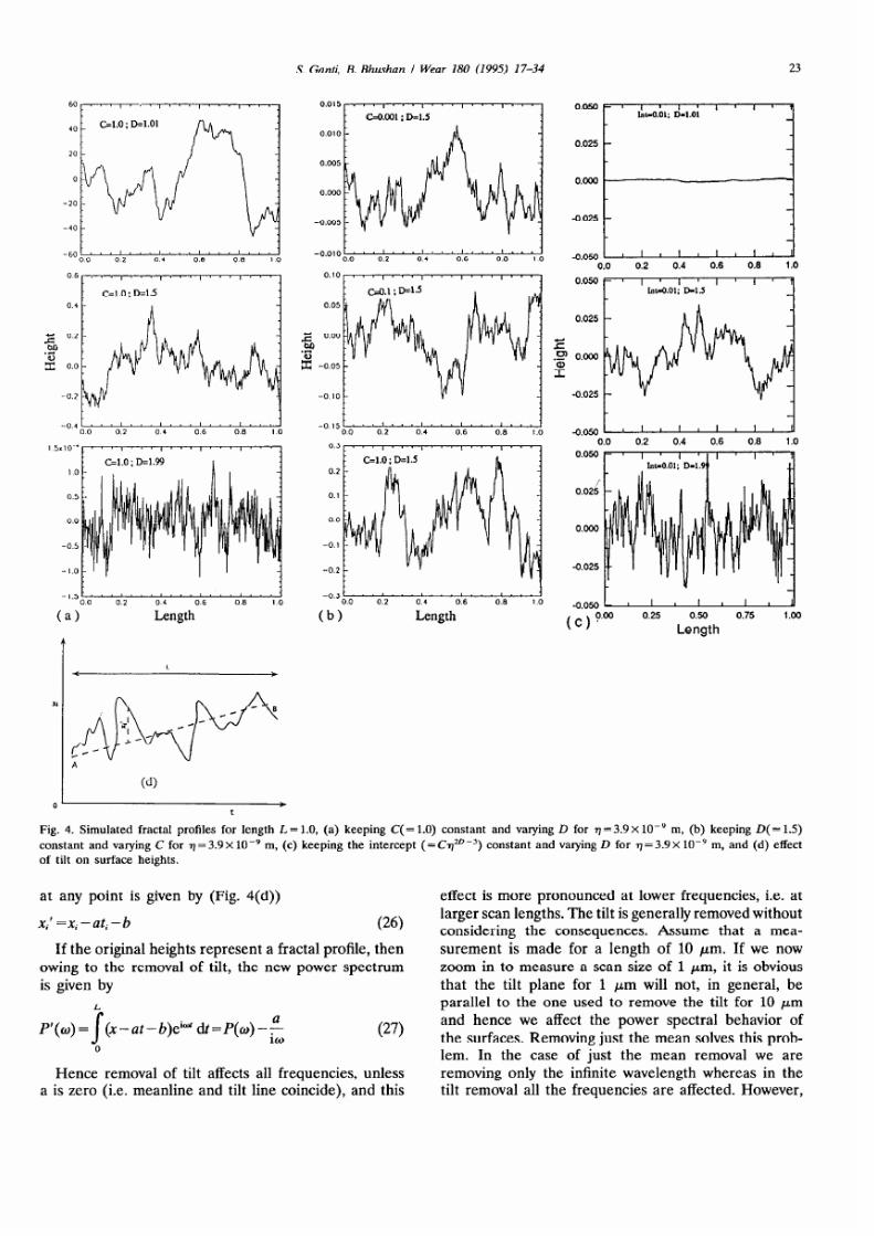
frequencies). Figs. 4(a) and 4(b) show the simulated

profiles for various Cs and D s. The increase in relative

power of higher frequencies with an increase in D can

be seen from Fig. 4(a). Higher values of D representa surface which appears to be rougher with an increase

in the power of high frequency variations. The variation

in the vertical scale arises because of the constant,

2o-3. For constant D , heights (amplitu des of all fre-

luency components) are proportional to CID (Eq. (21))

as can be seen from F ig. 4(b). It is importan t to note

that n can never become zero. In fact it is greater

than a particular value vc, below wh ich the fractal

definition no more ho lds. As 77 > q, and the number

of points of discretization becomes large, the influence

of n decreases and we believe Cqwm 3 approaches a

constant value similar to GDP’ in the modified W-M

function [7]. Hence in Fig. 4(c), the intercept CvD w3

is kept constant. It can be seen that as D increases,

the relative power of higher frequen cies of the surface

increases much more than the amplitude of all fre-

quencies (Fig. 4(a)), if the intercept is kept con stant.

It is important to note that a rough surface does not

necessarily mean higher D , because roughness (am-

plitude of the frequencies) is a function of both D an d

C. An increase in D primarily increases the relative

power of higher frequen cies and an increase in C

primarily increases the amp litude of all the frequencies

1291.

3 .1 . Va r i ance o f t he p ro f i l e

If we consider two surfaces, one in which the tilt is

removed and the other in which only the mean is

removed, it can be mathematically shown that both

these surfaces do not have the same power spectral

behavior unless the mean plane and tilt plane coincide.

Let x=at + b represent the equation of the tilt line AB

where t is along the scan length axis and x is the h eight

at any point. Hence after remov al of the tilt, the height

7/27/2019 1-s2.0-0043164894065454-main


S. Gad, B. Bhushan I Wear 180 (1995) 17-34 23

-1.500’ ’ ’ ’ 10.2 0.6 OS 10

(a) Glgth

0.025

-0.025

0.05

0.025

c’ 0.00

.F!$E

z -0.05.o, o.ooo

2

-0 IO -0.025

0.0 0.2 0 .4 0.6 0.6 1.0

0.050 1 , 8 , 1

I ts-0 .01: D- l .9I

, 8 , 8

-1.0 -0.025

-a,t.““““““‘.“.,i0.0 0.2 0.1 0.6 0,s 1 o

(b) Length

4

-0.050 -

( c ) ?.O” 0.25 0.50 0.75 1 .00

Length

Cd)

0’ a-t

Fig. 4. Sim ulated fractal profiles for length L = 1.0, (a) keeping C( = 1.0) constant and varying D for ~=3.9 X lOmy m, (b) keeping D( = 1.5)

constant and varying C for q= 3.9 X 10d9 m, (c) keeping the intercept (= Cq”)-‘) constant and varying D for q= 3.9 X 10m9 m, and (d) effect

of tilt on surface heights.

at any point is given by (Fig. 4(d))

xi’ =x,-ati-b (26)

If the original heights represent a fractal profile, then

owing to the removal of tilt, the new power spectrum

is given by

P’(w)=]@--at-b)eiY dt=P(w)-k

0

(27)

Hence removal of tilt affects all frequencies, unless

a is zero (i.e. meanlin e and tilt line coincide), and this

effect is more pronoun ced at lower frequencies, i.e. at

larger scan lengths. The tilt is generally removed withou tconsidering the consequences. Assume that a mea-

suremen t is made for a length of 10 pm. If we now

zoom in to measure a scan size of 1 pm, it is obvious

that the tilt plane for 1 pm w ill not, in general, be

parallel to the one use d to remove the tilt for 10 ,um

and hence w e affect the power spectral b ehavior of

the surfaces. Removing just the mean solves this prob-

lem. In the case of just the mean removal we are

removing only the infinite wavelength whereas in the

tilt removal all the frequencies are affected. H owever,

7/27/2019 1-s2.0-0043164894065454-main


24 S. Ganti, B. Bhushnn I Wear 180 (1995) 17-34

on the average th e power sp ectra still follow the power

law but the variance calculations are affected. This

effect is more pronou nced at larger scan lengths as

longer wavelengths have higher power.

The variance is the area un der the curve in the

power spectrum . For a profile of length L and number

of points of discretization N with mean remo ved, the

relation of the standa rd surface param eters to the fractalparameters D and C can be obtained from Eqs. (21),

(25a) and (25b) as

f(N,D)=&+&+&-+...+(N,2;S-ZD

f(N,D) is convergent VD < 2;

g(W)=&+&+-&+...+1

(N/2)3-w

g(N,D) is not convergent VD .

42=2Cqw-3m-w h(N,D)

(27T-w

h ( N ,D ) = +w +& + - & - + ...+1

(N /2 ) ’ -w

h (N ,D ) is not convergent VD .

(28)

(29)

(30)

The increase of the variance with scan length c an

be clearly seen from Eq. (20). In some measuring

instruments 77= L /N and in others it is hardware limited.

For a given measuring instrument, if the number of

points of discretization is constan t,

77aL (77=L/N)

and hence

t i a L (31a)

This result has been observed by Sayles and Thomas

[6]; also see Feder [25]. Similarly we find

d2a; (31b)

(31c)

4. Experimental procedure and data analysis

4.1. Test samp les and measurement techn iqu es

Measurements were made on a variety of sur-

faces - CrO , particulate magn etic tap es, thin-film mag -

netic rigid disks, steel disks (AISI 52100), high density

polyethylene (HDPE) plastic disks, hot filament chem-

ically vapor deposited (HFCVD ) diamond films. Mag-

netic tapes were prepared using a range of calendering

pressures resulting in a range of surface roughnesses

(Tapes A l-A6 in [5]). Magnetic disks were prepared

using as-polished and textured substrates with the same

construction as used for disk Bl in Bhushan [5]. AISI

52100 steel disks were hardened by heat treating at

955 “C for 1 h and oil tempered at 490 “C for 30 min.

The hardness of the hardened disk was about 63-64

HRC. T hese disks were mechanically polished w ithdifferent grades of polishin g paper (ranging from 80

to 600 grit size) followed by fine polishin g on velvet

cloth in the presence of diamond paste (0.25 pm) and

a lubricant. Roughest disks were only lapped with a

200 grit polishing paper. The plastic disks were rough-

ened by sliding against 120 and 250 grit polishing papers

in the presence of water. HF CVD diamond films used

in our study were as deposited and laser polished [30].

Surface roughness measurements are made primarily

by using two different instrum ents, a noncon tact optical

profiler (NOP) and an atomic force microscope (AFM)

at several lateral resolutions and scan lengths ranging

from 1 to 4000 pm [5]. Plastic disk s and diam ond filmswere too rough to be measured using the NOP . Hence

the data were taken only using the AFM.

For friction measurem ent of mag netic tap es, a re-

ciprocating friction apparatus was used. In this ap-

paratus, a 12.7 mm wide tape segment was reciprocated

over a polished Ni-Zn ferrite rod at a nominal tension

of 2.2 N and the coefficient of friction was measured

[5]. For friction m easurem ent of magn etic disks , a

magnetic disk drive was used. An Al,O,-TiC slider was

slid against the disk surface at a nominal load of 0.15

N (5 kPa) and 1 m s- ’ and the coefficient of friction

was measu red [5]. For friction measu rement of steel

and plastic d isks and diamond films, a ball-on-diskreciprocating friction apparatus was used. In this ap-

paratus, a ball with a diameter of 5 mm and a surface

finish of 2-3 nm rms (for a scan length of 250 pm

using the NOP), was slid in a reciprocating mode against

the sample at a reciprocating amplitude of 0.4 mm and

a frequency of 1 Hz [30 ]. For steel disk s, a 521 00 steel

(hardened) ball at 1 N load was used; for plastic disks,

the steel ball at 0.1 N was used; and for diamond films,

the alumina ball at 1 N was used. For p lastic disks,

lower loads were used to avoid ploughing.

7/27/2019 1-s2.0-0043164894065454-main


S. Gunti , B . Bhushan I Wear 180 (1995) 17-34 25

4 .2 . D a ta ana l y s t i

The data were analyzed using the structure and power

functions. For the calculation of structure function,

circular convolution is used over the set of discretized

data so as to keep the number of increments available

for averaging to remain the same. If the profile of

length L is discretized in N points,

h N t j = h j(32)

The power function is calculated by taking the FFT

on the discretized data. If h j an d H k represent the

Fourier pair,

(33a)

(33b)

and hence the power P k at frequency kfo where f. is

the fundam ental frequency is given by

P k = L I H k 1 2 (34)

The power functions along individual profiles showed

superpo sed variation on the general trend of power

law behavior, JezD [16]. Hence both the structure and

power functions along individual profiles are averaged

over all of the p rofiles to get a smoo th variation.

5. Results and discussion

Roughness data for various sam ples are presented

in Tables 1 and 2. Figs. 5-7 show selected surface

profiles for magn etic tape, mag netic disk and steel disk

surfaces. The TJ required for calculation of variance

and fractal parameters was the lateral resolution of

the measuring instrument. For the NOP it was 0.2 pmand 1 pm for 50 pm and 250 pm scan lengths re-

spectively. For AFM , it was scan length divided by the

number of data points (=25 6). Fig. 8 presents the

variance as a function of scan length for all samp les.

We generally note an increase in variance as a function

of scan length a s expected (from Eq . (28)) except for

the lower values obtained from the NOP at large scan

lengths which we cannot explain. The multi-scale be-

havior is reconfirmed from the data presented on the

described surfaces. It is observed that the surface

variance depends on the measurement technique and

the resolution of the instrument. Fig. 9(a) shows plotsof measured (+ and simulated c as a function of scan

length for tapes. If the s imulated (+ is plotted as a

function of measured u at a small scan length (Fig.

9(b)), the correlation is good.

Structure function plots for all sam ples are presented

in Figs. 10-14. It is observed that the structu re function

flattens out towards the end of increment size for each

scan length. W e speculate that it is because of the

following reason s: (1) the presence of minor scratche s

(or lay at the local level) disturbs the in-built char-

acteristic of self-affinity in the surfaces and decreases

the autocorrelation, (2) the removal of tilt from a fractal

Distance, urn

Fig. 5. Surface roughn ess profiles of a smooth magn etic tap e (tape 1) measured using the AFM and the NOP at different scan lengths.

Profiles (a), (b), and (c) were ob tained using the AFM and profile (d) was obtained using the NOP.

7/27/2019 1-s2.0-0043164894065454-main


26

Table 1

S. Gad, B. Bhushan / Wear 180 (1995) 17-34

Sur face parameters for magnetic media

Sample Scan size (PmXpm) g (nm) D C 6-d Simul ated v (nm)

Tape 1

Tape 2

Tape 3

Tape 4

M agnetic disk 1 (radial)

M agnetic disk 2 (radial)

1 (AFM)

10 (AFM)

50 (AFM)

100 (AF M )50 (NOP)

250 (NOP)

4000 (N OP )

1 (AFM)

10 (AFM)

50 (AFM)

100 (AF M )

50 (NOP)

250 (NOP)

1 (AFM)

10 (AFM)

50 (AFM)

100 (AF M )

250 (NOP)

1 (AFM)

10 (AFM)

50 (AFM)

100 (AF M )

250 (NOP)

1 (AFM)

10 (AFM)

50 (AFM)

100 (AF M )

50 (NOP)

250 (NOP)

4000 (NOP)

1 (AFM)

10 (AFM)

50 (AFM)

100 (AF M )

50 (NOP)

250 (NOP)

4000 (N OP )

3.9 1.42 0.13 1.6

18.9 1.21 0.20 10.4

20.2 1.27 0.26 21.0

21.0 1.26 0.16 30.021.6 1.20 0.54 14.45

15.2 1.23 0.02 45.5

22.7 1.30 2.6e-3 156.9

6.3 1.34 0.11 1.9

28.0 1.22 0.54 19.0

33.0 1.27 0.93 35.0

32.0 1.26 0.46 39.2

28.1 1.29 0.85 35.5

23.2 1.29 0.04 75.7

5.6 1.43 0.23 2.2

36.7 1.30 1.32 21.2

51.0 1.24 1.41 53.5

45.0 1.26 0.97 62.9

26.8 1.27 0.05 116.0

8.9 1.44 0.47 2.5

47.1 1.20 1.54 22.7

54.0 1.22 1.74 66.6

58.0 1.24 1.82 83.2

32.4 1.28 0.15 141.0

0.7 1.33 9.77e - 4 0.8

2.1 1.31 7.59e - 3 2.4

4.8 1.26 1.74e-2 5.6

5.6 1.30 1.38e - 2 6.3

3.5 1.27 1.58e-2 4.6

2.4 1.32 2.75e - 4 12.1

3.7 1.29 7.89e - 5 33.1

1.2 1.12 1.51e-2 0.8

8.4 1.39 1.99e-2 2.6

10.0 1.37 1.48e-2 5.8

11.0 1.32 6.91e - 2 9.8

10.0 1.34 l.l le-2 4.6

4.5 1.32 3.80e - 3 13.1

6.2 1.30 6.72e-4 39.0

AF M : atomic force microscope.

N OP: noncontact optical profiler.

surface changes the structure function of the surface,

and (3) the actual number of increments available for

averaging decreases. It is observed that the correlation

between the increments decreases rapidly towards the

end of the increment size and hence S(T) reaches a

value of twice the variance at that scan length. It was

suggested by Oden et al. (20) that the tape surface is

bifractal as the structure function at lower scan lengths

shows a trend suggesting a fractal dimension of 2. We

do not believe this argument as power law behavior

was again o bserved when w e go to higher scan lengths.

The values of D and C calculated from the structure

function (flat portion not included) are presen ted in

Tables 1 and 2. The variation in C within each su rface

is attributed to the simplified assumption of lateral

resolution of the measuring instrument as the intrinsic

length unit. Strong dependence of C on 77 and D can

be observed by an error analysis on the structure

function. We generally note that D does not change

very much for a given sample, however, C increases

monotonically with the variance of surface h eights for

a given measuring instrument. The NOP generally gives

lower values of C then does the AFM. Calculation of

C involves the use of n whose value is assumed to be

equal to the lateral resolution of the instrument.

It is possible for a surface to have different fractal

behavior in different regions, i.e. it might hav e different

fractal dimensions at different lengths (fractal regions).

For the four tapes measured, two distinct fractal regions

are observed-one at a scan length on the particle

7/27/2019 1-s2.0-0043164894065454-main


Table 2

S. Gad, B. Bhushan I Wear 180 (1995) 17-34 27

Surface parameters for engineering surfaces

Sample Scan size (PmXpm) c (nm) D C (nm) Simulated (T (nm)

Steel 1 (radial)

Steel 2 (radial)

Steel 3 (radial)

Plastic 1 (radial)

Plastic 2 (radial)

Plastic 3 (radial)

As-deposited diamond

Polished diamond

1 (AFM)

10 (AFM)

50 (AFM)

100 (AFM)50 (NOP)

250 (NOP)

4000 (NOP)

1 (AFM)

10 (AFM)

50 (AFM)

50 (NOP)

250 (NOP)

1 (AFM)

10 (AFM)

50 (AFM)

250 (NOP)

1 (AFM)

10 (AFM)50 (AFM)

100 (AFM)

1 (AFM)

10 (AFM)

50 (AFM)

100 (AFM)

1 (AFM)

10 (AFM)

50 (AFM)

100 (AFM)

1 (AFM)

10 (AFM)

50 (AFM)

100 (AFM)250 (NOP)

1 (AFM)10 (AFM)

50 (AFM)

100 (AFM)

1.2 1.39 6.90e-3 0. 6

2.9 1.45 1.82e - 2 1.9

4.5 1.45 1.41e-2 3.7

4.5 1.40 l.@e-2 4. 62.4 1.38 2.04e - 3 3.9

3.7 1.39 6.5Oe -4 8. 8

13.2 1.38 8.30e - 4 35.0

1.77 1.45 0.03 4.5

19.2 1.26 0.51 14.4

29.0 1.31 0.76 26.0

23.4 1.24 0.17 26.6

25.3 1.25 0.06 50.6

1.94 1.46 0.03 4. 5

20.7 1.48 0.69 17.1

67.6 1.38 0.85 37.7

79.9 1.37 0.97 78.8

10.2 1.49 0.81 3.6

60.9 1.29 1.32 53.6121.0 1.30 8.51 127.9

144.0 1.25 9.70 139.2

1. 5 1.46 0.02 21.5

107.0 1.41 12.0 61.9

242.0 1.36 16.6 158.9

283.0 1.33 13.5 224.3

20.0 1.42 2.45 11.9

157.0 1.46 4.68 33.6

302.0 1.47 8.51 78.6

442.0 1.47 7.10 125.4

41.0 1.38 8.12 51.3

231.2 1.29 20.4 159.1

482.6 1.25 38.9 348.3

537.8 1.28 47.8 508.8457.1 1.26 11.5 757.7

16.3 1.46 2.73 27.9

155.0 1.33 15.2 84.9

176.0 1.32 24.8 199.8

192.0 1.42 25.7 248.4

AFM: atomic force microscope.

NOP: noncontact optical profiler.

level and the other at higher scan lengths (Fig. 10).

The fractal dimen sion at 1 pm level (on the order of

the particle length) is the same for all the tapes (Table

1). This sugge sts th at the fractal dim ension of the

magn etic particles is about 1.4 (Particle size for thesetapes w as about 1 pm with an aspect ratio of 10.) The

fractal dim ension of the magn etic p article is larger than

that of the tape o n a larger s cale (relative powe r of

higher frequencies is high). All these tapes show the

same behavior in the longitudinal and transverse di-

rections. In fact the fractal d imens ions at large scan

lengths for all the tapes do not differ much from each

other and hence the roughness (a at 50 pm scan length)

is dependent mainly on the value of C. This can be

seen from Fig 15(a)(i).

Thin film magnetic disks both as polished and textured

show a fractal region when the scan length is sufficiently

sma ll (Fig. 11). In the radial direction perpend icular

to the texture, w avy form in the structure function is

observed as the texture is a compo sition of a fewfrequencies which have higher power relative to the

other frequencies. It is observed that for a frequency

higher than the dom inant textured frequency, the fractal

behavior is seen in the direction perpend icular to the

texture. As expected, the as polished disk is isotropic

in nature. The variation of C with variance is shown

in Fig. lS(a)(ii).

Three steel sam ples were hand polished to different

roughnesses. All the steel samples show a fractal be-

havior even to a scan length of 1 pm (Fig. 12). The

7/27/2019 1-s2.0-0043164894065454-main



. 1.00

o= 2.4nm

Distance, pm

Fig. 6. Surface roughness profiles of a smooth m agnetic d isk (magnetic disk 1) measured using the AFM and the NOP at different scan

lengths. Profiles (a), (b), and (c) were obtained using the AFM and profile (d) was obtained using the NOP.

0 = 1.2 nm

ii.C!?

o= 4.5 nm

5

8_50.0

::

Distance, Frn

Fig. 7. Surface rough ness profiles of a smooth steel disk (steel 1) measured using the AFM and the NOP at different scan lengths. Profiles

(a), (b), and (c) were obtained using the AFM and profile (d) was obtained using the NOP.

value of C increases with variance as can be seen from observed in the two directions. In the direction parallel

the Fig. lS(a)(iii). to the texture, the dimen sion is approximately 1.5 and

The sm ooth plastic sample is isotropic and hence hence is a case of Brow nian motion. There is no lateral

the same slope is observed for the structure function shift observed in the structure functions at different

in both directions (Fig. 13). The rough p lastic sample scan lengths as can be explained from the equation.

is textured in the circumferential direction and hence In the direction perpendicu lar to the textured frequency,

two different patterns for the structure function are the dimension observed is much lower than 1.5 and

7/27/2019 1-s2.0-0043164894065454-main



*’ (b )I I I ’ I I I I _

_____e ____- Mag.#jsk-1 -

---o-- Mag.dlsk-2 1

15 -

0

10 -)_-- x.

-t

Hf l . .. .

. .I

5 T_---a-..__ . .

Gl

_,_.p--- ----___----_._

3

.* ---__

0 I I I I I I I I100

80

60

40

20

0

400

300

200

10 0

60:

400

200

(c) ’I ’ I ’ I ’

--_A-------

_____e_____ !=&I+,

--*-- steal-2

I 3- - - staa’-3/ ,Mp-=-.____

.d ’ -_/’

I ’ I ’ I ’ I ’

- 63 ,+

/ _----:-; pw; -

/-e - FwrlG3

I I I t I t I I

I ’ II 1’1’1’ 1

i

Cd __Aof,

I

As dep.diamond

laser p&diamond

I

0I I I I I I I I

50 10 0 150 200 250

Scan length , pm

Fig. 8. Variation of measured u with scan length for (a) magnetic

tapes, (b) magnetic disks, (c) steel disks, (d) plastic disks, and (e)

diamond films.

25

E 75

i 50

5

6 25

0

(b )

20

Scat%ngth6P pm

80 100

I I I I I I I I I 81

20 40 60 80 100

Measured o , nm

Fig. 9. (a) Comparison of simulated and measured (r for tapes at

different scan lengths, and (b) comparison of simulated and measured

(r for tapes at 50 pm and 100 pm scan lengths.

hence a lateral shift is observed as expected. The av erage

variance in the direction parallel to the texture is much

lower than the variance for the overall sample. T hesimu lated profiles give a lower value of the 77 parallel

to the texture which ag rees with the average 71 alculated

in that direction. Fig. lS(a)(iv) show s the variation of

C with variance. Texture introduces low frequency

variations which raises the u value.

Diamond films (HFCVD ) are also observed to be

fractal in nature (Fig. 14). Even though the u values

are very high, the fractal dimen sion is around 1.2 (Table

2) showing that higher roughness does not necessarily

mean higher fractal dimension. Variation of C with

variance is shown in Fig. 15(a)(v). The data in Figs.

lS(a)(ii) and 15(a)(v) are insufficient for a definite

prediction but they seem to conform qualitatively to

the expected results.

The roughness u is dependent on the parameters D

and C as can be seen from E qs. (20) and (21). For

all the samples measured, the value of D did not vary

much and hence the variance shows a good correlation

with C for a given measuring instrument. This can be

seen from Fig . 15(b). The coefficient of friction p is

plotted again st C for each m aterial. It can be seen

that as C increases, friction coefficient w decreases for

tape and magnetic disk samples because the real area

7/27/2019 1-s2.0-0043164894065454-main


S. Gad, B. Bhushan I Wear 180 (1995) 17-34

/fyT=A

A+. .

(

,,-.t10.' 1o- 6 10-4 I o- 1

:

Cd),o-1’ _ o

,,.,,, I ,,,, ,,, d ,,,,A , ,Lryl , ,,,,,,,o-‘P

1o-8 1o- 6 10-4 1o- ’

Fig. 10. Structure function for the roughness data measured at various scan lengths for (a) tape 1, (b) tape 2, (c) tape 3, and (d) tape 4.

For roughness statistics, see Table 1.

Mag. disk- 1sg. disk-l

(a> x,m (b ) x,m

Fig. 11. Structure functions for the roughness data measured at various scan lengths for magnetic disks 1 and 2 in (a) radial direction, and

(b) tangential direction. Texturing was nearly tangential. For roughness statistics, see Table 1.

of contact decreases with an increase in u or C (5). to increase with an increase in C. This might be due

Data are insufficient in Figs. 16(b) and 16(e) for a to the ploughing action as the steel and diamond surfaces

definite prediction. In Figs. 16(c) and 16(e), p seems are hard. Since there is a good correlation between

7/27/2019 1-s2.0-0043164894065454-main



e:b+ .

d.

^10. "

P

Gz

lo - ‘8

0

0 (b)

1o- 6 1o-6 1o- ’ 10-1

,O.‘Oto,/,,, ,,,,,,,,,,,, ,,,,,,,, ,,,,,,, , ,,,,,J

&j1o-6 10-6 10“ lo-’

z,mFig. 12. Structure functions for the roughness d ata measured at

various scan lengths for (a) steel 1, (b) steel 2, and (c) steel 3. For

roughness statistics, see Table 2.

variance and C, the trends observed for p as a function

of C are sam e as for p as a function of u. Since C is

unique for a surface, it is more approp riate to study

friction in terms of the fractal param eter C.

6. Conclusions

Surfaces are modeled as nonstationary processes w ith

stationary incremen ts. These surfaces follow a pow er

law behavior for structure and power functions. The

structure and power functions with lateral resolution

taken into account are given by

S(7) =cTf-3T4-zD

P(0) =$-g

where

1c,= m C

s(1-cosx~-(5-~)dX

0

= I'(5 - 2D)sin[ 42 -D)] c

27 r

The new parameters D and C provide a machine-

independ ent parame trization. D represents the relative

power of the frequencies and C the amplitudes of all

frequencies. Variance of a surface heig hts is related

to D, C and the scan length L .

Based on the measured surfaces, it is observed that

almo st all isotropic engineering surfaces an d textured

surfaces can be represented as nonstationary processes

with stationary increments. Variances of the simulated

profiles show a good correlation with the measured

values. The theory agrees w ell for small scan lengthsbut for larger sc an lengths a departure is observed.

Varian ces are affected by the tilt removal. This effect

is more pronounced at larger scan lengths. This is the

reason for the variations observed for the measu red

values.

In the case of magnetic tapes, steel disks and diamond

films, the isotropic nature in the surface produc es similar

structure functions in the two perpend icular directions

(radial and circumferential in the case of disk s and

longitudinal and transverse in the case of tapes). H ow-

ever, in the case of textured magn etic and plastic disk s,

the anisotropy due to the texture gives rise to different

structure functions and hence different va lues of thefractal parame ters. How ever, when the frequencies

measu red are greater th an the texture frequencies, the

structure functions look similar in these two directions

sugg esting a similar ordered structure in that frequency

range. For each sample observed, the fractal dimension

D remained constan t (except in the particle or the

grain size region) but C increased as the variance is

increased for a given measu ring instrum ent. The vari-

ation in C within each surface is attributed to the

simplified assum ption of lateral resolution as the in-

trinsic length unit. The trend for the coefficient of

friction p as a function of C is similar to that for

variance. Since C in theory, is uniqu e for a surface,

whe reas variance is not, it is more app ropriate to

characterize a surface and friction with C.

Experime ntally, mod erate offset in the structure func-

tion obtained from roughness m easurements made using

different instrum ent resolutions, has been obtained .

Howev er, offset in the structure functions obtained

using the present G-B model with lateral resolution

as the intrinsic length unit is found to be significant.

Add itional work is needed to better define the intrinsic

length unit.

7/27/2019 1-s2.0-0043164894065454-main



Plastic - 1

1

(a> 7,m

10-‘1

10-I’

IO-”

lo-"

IO-”

lo-"

lo-’ 10-c 10.’ 10-z

10-6

10-1'10-a 10-6 1o- 4 lo-’

10-I’

10-15

Fig. 13. Structure functions for the roughness data measured at various scan lengths for plastic disks 1, 2 and 3 in (a) radial direction, and

(b) tangential direction. Texturing in the rough samples was nearly circumferential. For roughness statistics, see Table 2.

IO-”

10.’ 10-c 1o-4 10-Z I o-8 10-4 10-z

4,m

Fig. 14. Structure functions for the roughness data measured at various scan lengths for (a) as deposited diamond, and (b) polished diamond

films. For roughness statistics, see Table 2.

7/27/2019 1-s2.0-0043164894065454-main


S. Ganti, B. Bhushan I Wear 180 (1995) 17-34 33

0.6 I

- (4

0. 4 - 0

0

??0.2

(1-

0.0 I

0 1 20.6 I

- ( b)

0.4 -

0.2 - • J

0

E1

v-

0.0 ’ I I

0.000.6

F

(1

0 0.012 0.025

(c) 0

0.4

0.2Ix

F

0 50 10020 I

(i v) 0

0.0

0.6'

0.4

0.2

lol. ?? +-+---It I1

0 200 40080, I I

(VII)

40

i 1I

t0. 0 L

o.6mOL-- -- -J

0 250 500

(a)0, nm

0.4

t

60

C. nm

Fig. 16. Variation of the friction coefficient p with C at a scan length

of 50 pm for (a) magn etic tapes, (b) magnetic disks, (c) steel disks,

(d) plastic disks, and (e) diamond films.

Acknowledgements

(b) c,nm

This research was sponsored in parts by the De-

partment of the Navy/Office of the Chief of Naval

Research (Contract No . N00014-93 -l-0067), Advanced

Research Projects Agency/National Storage Industry

Consortium (Grant No. MD A 972-93-l-0009) and the

Ohio State University Fellowship (SG). We thank Dr.

Fig. 15. (a) Variation of C with c at a scan length 50 pm (Tables

1 and 2) for (i) magnetic tapes, (ii) magnetic disks, (iii) steel disks,

(iv) plastic disks, and (v) diamond films. (b) Variation of C with w

at a scan length of 50 pm (Tables 1 and 2) for ail the measured

samples.

7/27/2019 1-s2.0-0043164894065454-main


34 S. Ganti,

Vilas Koinkar for the AFM measurements

B.K. Gupta for the friction measurements.

Appendix A: Nomenclature

B. Bhushan ! Wear 180 (1995) 17-34

and Dr.

Im Hk

L

n1

PC4

fYw>

Re HkS(r)

-40

44

autocovariance function

amplitude coefficient

fractal dimension

fundamental frequency = l/L

scaling coefficient in W -M function

height at the jth node of the discretized profile

Fourier m ode corresponding to the frequency

kf0imaginary part of Hk

scan length of the profile

lower cut-off frequency of the measu red profile

probability distribution function

power spectral density function

real part of Hkstructure function

random process

height profile of the simulated profile

Greek letters

length parameter in fBm

discrete frequencies in W-M function

mean of the random process

lateral resolution of the instrum ent

frequency

increment in the structure function

variance of heights

variance of slopes

variance of curvatures

References

11 1

12 1

[31

[41

[51

[61

MS. Longuet-Higgins, Statistical properties of an isotropic

random surface, Phil os. Trans. R. Sot. L ondon, Ser. A, 250

(1957) 1.57-174.

P.R. Nayak, Random process model of rough surfaces, J. Lube.

Technol., 93 (1971) 39& 407.

T.R. Thomas, Rough Swjiices, Longman, New York, 1982.

J.A. Greenwood and J.B.P. Williamson, Contact of nominally

flat surfaces, Proc. R. Sot. Lon don, Ser. A, 295 (1966) 30& 319.

B. Bhushan, Tr ibol ogy and Mechanics of Magnetic Storage Devices,

Springer, New York, 1990.

R.S. Sayles and T.R. Thomas, Surface topography as a non-

stationary random process, Natire (London), 271(1978) 4311134.

[71

I81

[91

[lOI

1111

[121

[131

1141

[151

(161

[171

tl81

[191

[201

[211

[221

1231

v41

v51

[261

[271

[281

v91

[301

A. Majumdar and B. Bhushan, Role of fractal geometry in

roughness characterization and contact mechanics of surfaces,

ASME J. Tri boZ., 112 (1990) 205-216.

J.J. Gagnepain and C. Roques-Carries, Fractal approach to

two-dimensional and three-dimensional surface roughness,

Wear, 109 (1986) 119-126.

F.F. Ling, Fractals, engineering surfaces and tribology, Wear,

136 (1990) 141-156.

G.Y. Zhou, M.C. Leu and S.X. Dong, Measurement andassessment of topography of machined surfaces, in ES. Geskin

and S.V. Samarasekara (eds.), Mi crosmtctural Evolution in Metal

Processing, ASME, New York, 1990, pp. 89-100.

B.B. Mandelbrot, TheFractalGeomehyofNahtre, W.H. Freeman,

New York, 1983.

B.B. Mandelbrot, D.E. Passoja and A.J. Paullay, Fractal char-

acter of fracture surfaces of metals, Namre, 308 (1984) 721-722.

M. AIdissi, Fractals in conducting polymers, Adv. M ater., 4 (5)

(1992) 368-369.

M.V. Berry and Z.V. Lewis, On the Weierstrass-Mandelbrot

fractal function, Proc. R. Sot. L ondon, Ser. A, 370 (1980) 459-484.

K.J. Falconer, Dimensions- their determination and properties,

in J. Belair and S. Dubuc (eds.), Fr actal Geomehy and Anal ysis,

NATO AS1 Series, Kluwer, Dordrecht, 1989, pp. 221-254.

A. Majumdar and C.L. Tien, Fractal characterization and

simulation of rough surfaces, Wear, 136 (1990) 313-327.

A. Majumdar and B. Bhushan, Fractal model of elastic-plastic

contact between rough surfaces, ASME J. TriboZ., 113 (1991)

l-11.

A. Majumdar, B. Bhushan and C.L. Tien, Role of fractal

geometry in tribology, Adv. I nfo. Storage Syst., 1 (1991) 231-265.

B. Bhushan and A. Majumdar, Elastic-plastic contact model

for bifractal surfaces, Wear, 153 (1992) 53-64.

PI. Oden, A. Majumdar, B. Bhushan, A. Padmanabhan and

J.J. Graham, AFM imaging, roughness analysis and contact

mechanics of magnetic tape and head surfaces, ASME J. Tri bal.,

114 (1992) 666-674.

W.B. Davenport, Jr., ProbabiI ityandRandomPr ocesses, McGraw-

Hill, New York, 1970.

A.M. Yaglom, Correlati on i%eov of Stationary and Related

Random Functions I -Basic Results, Springer, New York, 1987.A. Papoulis, Probabil ity, Ran dom Vari ables and Stochastic Pr o-

cesses, McGraw-Hill, New York, 1965.

T. Hida, Brownian Motion, Springer, New York. 1980.

J. Feder, Fractak, Plenum, New York, 1988.

W. Rumelin, Simulation of fractional Brownian motion, in H.O.

Peitgen, J.M. Henriques and L.F. Penedo (eds.), Proc. 1st. IF IP

Conf: on Fr actals in the Fu ndamental and Appli ed Sciences, 1991,

pp. 379-393.

R.F. Voss, Random fractals: Characterization and measurement,

in R. Pynn and A. Skjeltorp (eds.), Scaling Phenomena in

Dirordered Systems, NATO AS1 series, KIuwer, Dordrecht, 1985,

pp. 1-12.

D.L. Turcotte, Fr actal and Chaos in Geology an d Geophysics,

Cambridge University Press, New York, 1992.

S. Ganti, Generalized fractal analysis and its applications to

engineering surfaces, M.S. nesis, Department of Mechanical

Engineering, The Ohio State University, Columbus, OH, No-

vember 1993.

B. Bhushan, V.V. Subramaniam, A. Malshe, B.K. Gupta and

J. Ruan, Tribological properties of polished diamond films, .I.

Appl. Phys., 74 (1993) 41744180.

1-s2.0-0043164894065454-main

Documents