Transportation Research Part B 45 (2011) 1177–1189

Contents lists available at ScienceDirect

Transportation Research Part B

journal homepage: www.elsevier .com/ locate/ t rb

Robust optimization for emergency logistics planning: Risk mitigationin humanitarian relief supply chains

Aharon Ben-Tal a, Byung Do Chung b, Supreet Reddy Mandala b, Tao Yao b,⇑a Faculty of Industrial Engineering and Management, MINERVA Optimization Center, Technion – Israel Institute of Technology, Technion City, Haifa 32000, Israelb The Harold & Inge Marcus Department of Industrial and Manufacturing Engineering, Pennsylvania State University, University Park, PA 16802, USA

a r t i c l e i n f o

Keywords:Robust optimization

Dynamic traffic assignmentDemand uncertaintyEmergency logistics

0191-2615/$ - see front matter � 2010 Elsevier Ltddoi:10.1016/j.trb.2010.09.002

⇑ Corresponding author.E-mail addresses: abental@ie.technion.ac.il (A. Be

a b s t r a c t

This paper proposes a methodology to generate a robust logistics plan that can mitigatedemand uncertainty in humanitarian relief supply chains. More specifically, we applyrobust optimization (RO) for dynamically assigning emergency response and evacuationtraffic flow problems with time dependent demand uncertainty. This paper studies a CellTransmission Model (CTM) based system optimum dynamic traffic assignment model.We adopt a min–max criterion and apply an extension of the RO method adjusted todynamic optimization problems, an affinely adjustable robust counterpart (AARC)approach. Simulation experiments show that the AARC solution provides excellent resultswhen compared to deterministic solution and sampling based stochastic programmingsolution. General insights of RO and transportation that may have wider applicability inhumanitarian relief supply chains are provided.

� 2010 Elsevier Ltd. All rights reserved.

1. Introduction

Over the past three decades, the number of reported disasters have risen threefold. Roughly, 5 billion people have beenaffected by disasters with an estimated damages of about 1.28 trillion dollars (Guha-Sapir et al., 2004). Although most ofthese disasters could not have been avoided, significant improvements in death counts and reported property losses couldhave been made by efficient distribution of supplies. The supplies here could mean personnel, medicine and food which arecritical in emergency situations. The supply chains involved in providing emergency services in the wake of a disaster arereferred to as humanitarian relief supply chains. Humanitarian relief supply chains are formed within short time period aftera disaster with the government and the NGO’s being the major drivers of the supply chain. Clearly, emergency logistics is animportant component of humanitarian relief supply chains.

Most literature in emergency logistics focuses on generating transportation plans for rapid dissemination of medical sup-plies inbound to the disaster hit region (Sheu, 2007; Ozdamar et al., 2004; Lodree and Taskin, 2008). There is, however, an-other aspect of emergency logistics which is often ignored – outbound logistics. The outbound logistics considers a situationwhere people and emergency supplies (e.g. medical facilities and services for special need evacuees) need to be sent from aparticular location affected by disaster within a given time horizon.

In the outbound emergency logistics, the demand of traffic flows is usually highly uncertain and depends on a number offactors including the nature of disaster (natural/man-made) and time of impact. This uncertainty in the demand causes dis-ruptions in emergency logistics and hence disruptions in humanitarian relief supply chains leading to severe sub-optimalityor even infeasibility which may ultimately lead to loss of life and property. In order to mitigate the risk of uncertain demand,

. All rights reserved.

n-Tal), buc139@psu.edu (B.D. Chung), sxm529@psu.edu (S.R. Mandala), taoyao@psu.edu (T. Yao).

1178 A. Ben-Tal et al. / Transportation Research Part B 45 (2011) 1177–1189

we study the problem of generating evacuation transportation plans which are robust to uncertainty in outgoing demand.More specifically, we solve a dynamic (multi-period) emergency response and evacuation traffic assignment problem withuncertain demand at source nodes.

Researchers and practitioners in the field of transportation are concerned with multi-period management problems withan inherent time dependent information uncertainty. Traditional dynamic optimization approaches for dealing with uncer-tainty (e.g. stochastic and dynamic programming) usually require the probability distribution for the underlying uncertaindata to obtain expected objectives. However, in many cases, it may be very difficult to accurately identify the distributionrequired to solve a problem. Especially, this is more likely true when we are considering an evacuation transportation prob-lem due to the inherent complexity and uncertainty. In addition, the robust solution guaranteeing the feasible evacuationplan is important since infeasible solutions may cause the potential loss of life and property in extreme events.

We explore the potential of robust optimization (RO) as a general computational approach to manage uncertainty, fea-sibility, and tractability for complex transportation problems. RO approach has been originally developed to deal with staticproblems formulated as linear programming (LP) or conic-quadratic problems (CQP), using crude uncertainty with hard con-straints. It means that uncertainty is assumed to reside in an appropriate set and RO guarantees the feasibility of the solutionwithin the prescribed uncertainty set by adopting a min–max approach. The RO technique has been successfully applied insome complex and large scale engineering design and optimization problems similar as robust control in control theory(Ben-Tal and Nemirovski, 1999, 2002).

The original RO approach considers static problems. The underlying assumption of RO is ‘‘here and now” decisions, and alldecision variables need to be determined before any uncertain data are realized. This is not typical in many transportationmanagement problems that have the multi-period nature. In multi-period transportation problems such as dynamic trafficassignment, ‘‘wait and see” decisions are made, which means some decision variables are ‘‘adjustable” and affected by part ofthe realized data. Recognizing the need to account for such dynamics, Ben-Tal et al. (2004) have extended the RO approachand developed an affinely adjustable robust counterpart (AARC) approach to consider ‘‘wait and see” decisions.

To demonstrate the use of AARC to emergency transportation management settings, in this paper we consider a systemoptimum dynamic traffic assignment (SO-DTA) problem. The main contributions of this paper are summarized as follows:

� This paper develops a robust optimization framework for system optimum dynamic traffic assignment problems. Theframework incorporates a linear programming (LP) formulation based on the Cell Transmission Model (CTM) (Daganzo,1993, 1995; Ziliaskopoulos, 2000) and the AARC approach by considering dynamical adjustments to realizations of uncer-tainty with appropriate uncertainty sets. The framework is converted to LP and hence computationally tractable.� This paper applies the proposed robust optimization framework to an emergency response and logistics planning prob-

lem. Numerical examples are provided to illustrate the value of the robust optimization in the context of emergency logis-tics and demonstrate the computational viability of the developed framework. Simulation experiments show that theAARC solution provides excellent results when compared to with the solutions of deterministic LP and Monte Carlo sam-pling based stochastic programming.� This paper obtains some general insights that may have wider applicability for transportation managers: (1) A robust

solution may improve both feasibility and performance when infeasibility costs are significant. Intuitively, the usual nom-inal optimal solution may be not far from the robust solution, but the usual optimal solution can perform much worse inthe worst case. (2) An integration of RO and transportation modeling will improve the generation, communication, andpotential use of uncertainty data in logistics transportation management. The intuition for this insight is twofold. First, inmany applications in transportation, the set-based uncertainty (used by RO) is the most appropriate notion of data uncer-tainty. Second, computational tractability (resulting from this set-based uncertainty and dynamic traffic flow modeling inLP formulations) lead to efficient solutions for logistics transportation management under uncertainty.

The structure of the paper is as follows. In Section 2, we provide a literature review. Section 3 presents a deterministicLP model for the CTM based SO-DTA problem. In Section 4, AARC is formulated by considering appropriate demand uncer-tainty sets. We study applications in evacuation transportation and provide experiment results for two emergency logisticsplanning examples in Section 5. Section 6 concludes and discusses future work.

2. Literature review

The DTA problem describes a traffic system with time-varying flow and has been studied substantially since the seminarwork of Merchant and Nemhauser (1978a,b). The main research can be classified into four categories: mathematical pro-gramming, optimal control, variational inequality, and simulation-based approach (see Peeta and Ziliaskopoulos (2001),Friesz and Bernstein (2000) for a review).

Daganzo (1993), Daganzo (1995) proposed the CTM model, consisting of a set of linear difference equations, to develop atheoretical framework to simulate network traffic. It was assumed that the best route from origin to destination are alreadyknown to the travellers. Ziliaskopoulos (2000) relaxed this assumption by formulating a single destination SO-DTA problemas a linear program with the decision variables being the route choices. Recently, the deterministic CTM based DTA modelhas been applied to evacuation management (e.g., Tuydes (2005), Chiu et al. (2007), Xie et al. (2010)). For example, Chiu et al.

A. Ben-Tal et al. / Transportation Research Part B 45 (2011) 1177–1189 1179

(2007) proposed a network transformation and demand modeling technique for solving an evacuation traffic assignmentplanning problem using the CTM based single destination SO-DTA model.

Recognizing that deterministic demand or network characteristics are unrealistic in some settings, another wave of re-search on DTA is modeling of stochastic properties and developing robust solutions. Waller et al. (2001), Waller andZiliaskopoulos (2006) addressed the impact of demand uncertainty and the importance of robust solution. Peeta and Zhou(1999) used Monte Carlo simulation to compute a robust initial solution for a real-time online traffic management system.Chance constraint programming for the SO-DTA problem is analyzed by Waller and Ziliaskopoulos (2006). Yazici and Ozbay(2007) introduced probabilistic capacity constraint and solved the CTM based SO-DTA problem for a hurricane evacuationproblem. Karoonsoontawong and Waller (2007) proposed a DTA based network design problem formulated as a two stagestochastic programming and a scenario-based robust optimization (Mulvey et al., 1995). Ukkusuri and Waller (2008) pro-posed a two stage stochastic programming with recourse model to account for demand uncertainty.

Recently, robust optimization has witnessed a significant growth (Ben-Tal and Nemirovski, 1998, 1999, 2000; El Ghaouiet al., 1997, 2003; Bertsimas and Sim, 2003, 2004). For a summary of the state of art in RO, please refer to Ben-Tal et al.(2009), Bertsimas et al. (2007) and references therein. RO has been proposed to apply in network and transportation systems(Bertsimas and Perakis (2005), Ordóñez and Zhao (2007), Atamturk and Zhang (2007), Mudchanatongsuk et al. (2008), Ereraet al. (2009), Yin et al. (2008), Yin et al. (2009) to name a few). Related to our work, Atamturk and Zhang (2007) propose arobust optimization approach for two stage network flow and design. Erera et al. (2009) develop a two-stage robust optimi-zation approach for repositioning empty transportation resources. Both of the studies are in the spirit of Ben-Tal et al. (2004)where the second stage variables are determined as recourse or recovery actions while maintaining feasibility after theuncertain data is realized.

3. CTM for the DTA problem

In this section, we summarize and reformulate the prior work on the deterministic linear program (DLP) based on thetraditional CTM model (Ziliaskopoulos, 2000). The CTM, named by Daganzo (1993, 1995), models freeway traffic flow usingsimple difference equations. It approximates the kinematic wave model under the assumption of a piecewise linear relation-ship between flow and density on the link. More formally, the following equation shows the relationship between trafficflow, q, and density on a link, k, in a traffic network.

q ¼minðvk; qmax;wðkmax � kÞÞ;

where v is free flow velocity, kmax is maximum possible density, w is backward wave speed and qmax is maximum allowableflow on the link.

The LP based CTM model of Ziliaskopoulos (2000) is a simplification of the original CTM model. In the CTM model, a seg-ment of a freeway is decomposed into cells based on the free flow velocity and length of discrete time step. By this division,vehicles can move only to adjacent cells in unit time. The connectors between cells are dummy arcs indicating the directionof flow between cells. The demand of the CTM model represents the vehicular trips for each OD pair. In other words, eachdemand has its own origin and destination node in the network. The demand for each OD pair is assumed to be known at thebeginning and used as input data of the CTM model. However, in our model, demand at the source node is uncertain.

We provide the reformulation of the deterministic LP based CTM model. The model includes the characteristics of time-space dependent cost and an adjacent matrix. In the traditional CTM research, it is assumed that the coefficient of cost is aconstant value within the time-space network. However, in this paper, the coefficient is assumed to be dependent on timehorizon and demand nodes. It is a more common situation and is necessary to study emergency logistics management. Anadjacency matrix A = [aij] is defined for representing the connectivity of the cells. The value of aij is equal to 1 if cell i is con-nected to cell j, otherwise aij = 0.

Based on the notations in Table 1, we present the deterministic linear programming (DLP) model:

minx;y

Xt2I

Xi2CnCs

cti x

ti ðM-DLPÞ ð1Þ

s:t:

xti � xt�1

i �Xk2C

akiyt�1ki þ

Xj2C

aijyt�1ij P dt�1

i ; 8 i 2 C; t 2 I ð2ÞXk2C

akiytki 6 Qt

i ; 8 i 2 C; t 2 I ð3ÞXk2C

akiytki þ dt

i xti 6 dt

i Nti ; 8 i 2 C; t 2 I ð4Þ

Xj2C

aijytij 6 Q t

i ; 8 i 2 C; t 2 I ð5ÞXj2C

aijytij � xt

i 6 0; 8 i 2 C; t 2 I ð6Þ

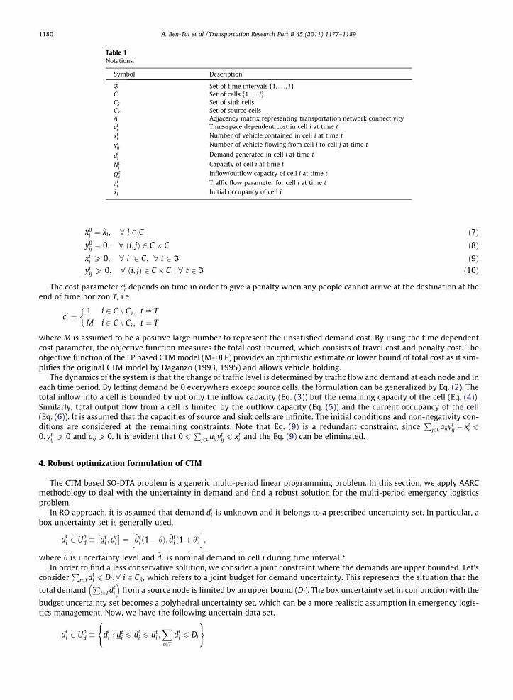
Table 1Notations.

Symbol Description

I Set of time intervals {1, . . . ,T}C Set of cells {1 . . . , I}CS Set of sink cellsCR Set of source cellsA Adjacency matrix representing transportation network connectivityct

i Time-space dependent cost in cell i at time t

xti Number of vehicle contained in cell i at time t

ytij Number of vehicle flowing from cell i to cell j at time t

dti

Demand generated in cell i at time t

Nti

Capacity of cell i at time t

Qti

Inflow/outflow capacity of cell i at time t

dti

Traffic flow parameter for cell i at time t

x̂i Initial occupancy of cell i

1180 A. Ben-Tal et al. / Transportation Research Part B 45 (2011) 1177–1189

x0i ¼ x̂i; 8 i 2 C ð7Þ

y0ij ¼ 0; 8 ði; jÞ 2 C � C ð8Þ

xti P 0; 8 i 2 C; 8 t 2 I ð9Þ

ytij P 0; 8 ði; jÞ 2 C � C; 8 t 2 I ð10Þ

The cost parameter cti depends on time in order to give a penalty when any people cannot arrive at the destination at the

end of time horizon T, i.e.

cti ¼

1 i 2 C n Cs; t – T

M i 2 C n Cs; t ¼ T

�

where M is assumed to be a positive large number to represent the unsatisfied demand cost. By using the time dependentcost parameter, the objective function measures the total cost incurred, which consists of travel cost and penalty cost. Theobjective function of the LP based CTM model (M-DLP) provides an optimistic estimate or lower bound of total cost as it sim-plifies the original CTM model by Daganzo (1993, 1995) and allows vehicle holding.

The dynamics of the system is that the change of traffic level is determined by traffic flow and demand at each node and ineach time period. By letting demand be 0 everywhere except source cells, the formulation can be generalized by Eq. (2). Thetotal inflow into a cell is bounded by not only the inflow capacity (Eq. (3)) but the remaining capacity of the cell (Eq. (4)).Similarly, total output flow from a cell is limited by the outflow capacity (Eq. (5)) and the current occupancy of the cell(Eq. (6)). It is assumed that the capacities of source and sink cells are infinite. The initial conditions and non-negativity con-ditions are considered at the remaining constraints. Note that Eq. (9) is a redundant constraint, since

Pj2Caijyt

ij � xti 6

0; ytij P 0 and aij P 0. It is evident that 0 6

Pj2Caijyt

ij 6 xti and the Eq. (9) can be eliminated.

4. Robust optimization formulation of CTM

The CTM based SO-DTA problem is a generic multi-period linear programming problem. In this section, we apply AARCmethodology to deal with the uncertainty in demand and find a robust solution for the multi-period emergency logisticsproblem.

In RO approach, it is assumed that demand dti is unknown and it belongs to a prescribed uncertainty set. In particular, a

box uncertainty set is generally used.

dti 2 Ub

d � dti ;

�dti

� �¼ ~dt

i ð1� hÞ; ~dti ð1þ hÞ

h i;

where h is uncertainty level and ~dti is nominal demand in cell i during time interval t.

In order to find a less conservative solution, we consider a joint constraint where the demands are upper bounded. Let’sconsider

Pt2T dt

i 6 Di;8 i 2 CR, which refers to a joint budget for demand uncertainty. This represents the situation that the

total demandP

t2T dti

� �from a source node is limited by an upper bound (Di). The box uncertainty set in conjunction with the

budget uncertainty set becomes a polyhedral uncertainty set, which can be a more realistic assumption in emergency logis-tics management. Now, we have the following uncertain data set.

dti 2 Up

d � dti : dt

i 6 dti 6

�dti ;Xt2T

dti 6 Di

( )

A. Ben-Tal et al. / Transportation Research Part B 45 (2011) 1177–1189 1181

Next, a specific form of linear decision rules is assumed to convert M-DLP to AARC formulation. The linear rules are usedto derive a computationally tractable problem by approximating the robust solution. We note that the solution from AARC isoptimal in worst case from the predetermined uncertainty set. However, there is no guarantee that the robust solution isclose to optimal in the other cases since the relationship between uncertain parameters and decision variables may notbe linear. Specifically, the adjustable control variables, yt

ij, can be represented as an affine function of previously observeddemand values, i.e., yt

ij ¼ p�1ijt þ

Ps2CR

Ps2It

pssijtd

ss , where p�1

ijt and pssijt are non-adjustable variables and It = {0,. . .,t � 1}.

Along with the affine rule of control variables, the state variables also becomes a affine function of the previously realizeddata, xt

i ¼ g�1it þ

Ps2CR

Ps2It

gssit ds

s , by the linear structure of CTM model.By substituting the state and control variables, we have the following AARC formulation:

minr;p�1 ;p;g�1 ;g

z ðM � AARCÞ

s:t:

Xt2I

Xi2C

cti g�1

it þXs2CR

Xs2It

gssit ds

s

!6 z; 8 dt

i 2 Ud

g�1it þ

Xs2CR

Xs2It

gssit ds

s

!� g�1

it�1 þXs2CR

Xs2It�1

gssit�1ds

s

!�Xk2C

aki p�1kit�1 þ

Xs2CR

Xs2It�1

psskit�1ds

s

!

þXj2C

aij p�1ijt�1 þ

Xs2CR

Xs2It�1

pssijt�1ds

s

!P dt�1

i ; 8 i 2 C; t 2 I

Xk2C

aki p�1kit þ

Xs2CR

Xs2It

psskitd

ss

!6 Qt

i ; 8 dti 2 Ud; i 2 C; t 2 I

Xk2C

aki p�1kit þ

Xs2CR

Xs2It

psskitd

ss

!þ dt

i ðg�1it þ

Xs2CR

Xs2It

gssit ds

s Þ 6 dti N

ti ; 8 dt

i 2 Ud; i 2 C; t 2 I

Xj2C

aij p�1ijt þ

Xs2CR

Xs2It

pssijtd

ss

!6 Q t

i ; 8 dti 2 Ud; i 2 C; t 2 I

Xj2C

aij p�1ijt þ

Xs2CR

Xs2It

pssijtd

ss

!� ðg�1

it þXs2CR

Xs2It

gssit ds

s Þ 6 0; 8 dti 2 Ud; i 2 C; t 2 I

g�1i0 ¼ x̂i; 8 i 2 C

p�1ij0 ¼ 0; 8 ði; jÞ 2 C � C

p�1ijt þ

Xs2CR

Xs2It

pssijtd

ss P 0; 8 ði; jÞ 2 C � C; t 2 I; dt

i 2 Ud

ð11Þ

The formulation (M-AARC) is intractable since it is a semi-infinite program, and it can be reformulated as a tractable opti-mization problem as shown in Theorem 1. The minimum objective value z, denoted as z�AARC , is a guaranteed upper boundvalue for all realization of uncertain data under the assumption of linear dependency. The objective value, z�AARC , also canbe interpreted as the optimistic estimate of total travel cost in worst case, which can be lower than the optimistic estimatefrom robust counterpart(RC), z�RC as AARC has a larger robust feasible region (Ben-Tal et al., 2004). The decision variables ofAARC are not adjustable control and state variables (yt

ij and xti , respectively), but a set of coefficient of affine function of the

control variables including p�1ijt ; pss

ijt ; g�1it and gss

it . It means that the solution of AARC is the linear decision rule. Specific val-ues of yt

ij and xti are calculated after the realization of the demand at time t � 1.

Theorem 1. Given polyhedral uncertainty set, Upd, the affinely adjustable robust counterpart of the CTM based SO-DTA problem

becomes the following linear programming problem and thus computationally tractable. Note that k is a set of dual variables andthe numerical indexes are used for notational simplicity.

minz;g;p;k

z ðM-AARC1Þ

s:t: Xs2I

Xs2CR

�dss k

11ss � ds

s k12ss

� �þXs2CR

Dsk13s 6 z�

Xt2I

Xi2CnCs

ctig�1it

k11ss � k12

ss þ k13s ¼

Xt¼fsþ1...Tg

Xi2CnCs

ctig

ssit ; 8 s ¼ f0; . . . T � 1g; s 2 CR

k11ss � k12

ss þ k13s ¼ 0; 8 s ¼ fTg; s 2 CR

k11ss ; k

12ss ; k

13s P 0; 8 s ¼ fTg; s 2 CR

1182 A. Ben-Tal et al. / Transportation Research Part B 45 (2011) 1177–1189

Xs2I

Xs2CR

�dss k

21itss � ds

s k22itss

� �þXs2CR

Dsk23its 6 g�1

it � g�1it�1 �

Xk2C

akip�1kit�1 þ

Xj2C

aijp�1ijt�1; 8 i 2 C; t 2 I

k21itss � k22

itss þ k23its ¼ Ifs¼t�1;s¼ig � gss

it þ ðgssit�1 þ

Xk2C

akipsskit�1 �

Xj2C

aijpssijt�1ÞIfs<t�1g;

8 s ¼ f0 . . . t � 1g; s 2 CR; i 2 C; t 2 I

k21itss � k22

itss þ k23its ¼ 0; 8 s ¼ ft . . . Tg; s 2 CR; i 2 C; t 2 I

k21itss; k

22itss; k

23its P 0; 8 s ¼ ft . . . Tg; s 2 CR; i 2 C; t 2 IX

s2I

Xs2CR

�dss k

31itss � ds

s k32itss

� �þXs2CR

Dsk33its 6 Q t

i �Xk2C

akip�1kit ; 8 i 2 C; t 2 I

k31itss � k32

itss þ k33its ¼

Xk2C

akipsskit ; 8s ¼ f0 . . . t � 1g; s 2 CR; i 2 C; t 2 I

k31itss � k32

itss þ k33its ¼ 0; 8 s ¼ ft . . . Tg; s 2 CR; i 2 C; t 2 I

k31itss; k

32itss; k

33its P 0; 8 s ¼ ft . . . Tg; s 2 CR; i 2 C; t 2 IX

s2I

Xs2CR

ð�dss k

41itss � ds

s k42itssÞ þ

Xs2CR

Dsk43its 6 dt

i ðNti � g�1

it Þ �Xk2C

akip�1kit ; 8 i 2 C; t 2 I

k41itss; k

42itss; k

43its P 0; 8 i 2 C; t 2 IX

s2I

Xs2CR

�dss k

51itss � ds

s k52itss

� �þXs2CR

Dsk53its 6 Q t

i �Xj2C

aijp�1ijt ; 8 i 2 C; t 2 I

k51itss � k52

itss þ k53its ¼

Xj2C

aijpssijt ; 8 s ¼ f0 . . . t � 1g; s 2 CR; i 2 C; t 2 I

k51itss � k52

itss þ k53its ¼ 0; 8 s ¼ ft . . . Tg; s 2 CR; i 2 C; t 2 I

k51itss; k

52itss; k

53its P 0; 8 s ¼ ft . . . Tg; s 2 CR; i 2 C; t 2 IX

s2I

Xs2CR

ð�dss k

61itss � ds

s k62itssÞ þ

Xs2CR

Dsk63its 6 g�1

it �Xj2C

aijp�1ijt ; 8 i 2 C; t 2 I

k61itss � k62

itss þ k63its ¼

Xj2C

aijpssijt � gss

it ; 8 s ¼ f0 . . . t � 1g; s 2 CR; i 2 C; t 2 I

k61itss � k62

itss þ k63its ¼ 0; 8 s ¼ ft . . . Tg; s 2 CR; i 2 C; t 2 I

k61itss; k

62itss; k

63its P 0 8 s ¼ ft . . . Tg; s 2 CR; i 2 C; t 2 IX

s2I

Xs2CR

ð�dss k

71ijtss � ds

s k72ijtssÞ þ

Xs2CR

Dsk73ijts 6 p�1

ijt ; 8 i; jð Þ 2 C � C; t 2 I

k71ijtss � k72

ijtss þ k73ijts ¼ �pss

ijt; 8 s ¼ f0 . . . t � 1g; s 2 CR; ði; jÞ 2 C � C; t 2 I

k71ijtss � k72

ijtss þ k73ijts ¼ 0; 8 s ¼ ft . . . Tg; s 2 CR; ði; jÞ 2 C � C; t 2 I

k71ijtss; k

72ijtss; k

73ijts P 0; 8 s ¼ ft . . . Tg; s 2 CR; i; jð Þ 2 C � C; t 2 I

g�1i0 ¼ x̂i; 8 i 2 C

p�1ki0 ¼ 0; 8 ði; jÞ 2 C � C ð12Þ

Proof. By using the following relationship, we can reformulate each constraint affected by uncertain data as an equivalentLP problem.

X

s2It

asi ds

i 6 v 8 dti 2 Ud ¼ dt

i < dti <

�dti ;Xt2T

dti 6 Di

( )

() maxds

i

Xs2It

asi ds

i

!6 v

Without loss of generality, the polyhedral uncertainty set is represented as Ad 6 b and maxdsi

Ps2It

asi ds

i

� �is written as (P). By

applying strong duality property, we can derive an equivalent constraint with dual problem (D) on the left hand side(Bertsimas and Sim, 2004).

max ad 6 v ðPÞ () min bk 6 v ðDÞs:t s:t

Ad 6 b ATk ¼ ad P 0 k P 0

A. Ben-Tal et al. / Transportation Research Part B 45 (2011) 1177–1189 1183

Therefore, there exists k satisfying bk 6 v,AT k = a and k P 0 and the equivalent AARC of the CTM based SO-DTA becomestractable. h

5. Emergency logistics management

Emergency management is one of the best application areas for applying robust optimization due to the uncertainty ofhuman beings and disaster. Robust solution, especially AARC solution, can play an important role for emergency logisticsplanning for several reasons. First of all, the role of hard constraint is emphasized since the penalty cost for an infeasiblesolution is loss of life or property. Next, it is very difficult to estimate or forecast the demand model in the to-be-affectedareas due to unexpected human behavior and nature of disaster. Finally, we can take advantage of updated or realized dataon demand by employing AARC solution. When we solve M-AARC1, the optimal coefficients of the Linear Decision Rule (LDR)are computed offline. Going online, the actual decision variables (flows) are determined for period t by inserting the revealeduncertainties from previous periods in the LDR. A fully online version of the method can be also implemented. In such ver-sion, at period t only the t-period design variables are activated. The horizon is then rolled forward and the problem is re-solved after adjusting the state variables revealed in previous periods.

In this section, an emergency logistics planning problem is considered and the meaning of demand uncertainty sets isexplained. Then, we present a summary of experiments to test the performance of the AARC approach. The AARC solutionis benchmarked against an ideal solution with complete future information, deterministic LP, and sampling based stochasticprogramming. Two test networks are chosen from Chiu et al. (2007) and Yazici and Ozbay (2007) for the numerical analysis.

5.1. Demand modeling

In an emergency logistics problem, a general approach to model time-varying evacuee demand is captured by the follow-ing steps: the first step of demand modeling is calculation of total demand. Next, demand arrival or vehicle departure rate isdetermined for describing a dynamic environment. For example, S-shape curve can be used for representing cumulativepercentage of demand arrival. In most studies, it is assumed that the parameters (e.g. slope) of S-curve are unknown butdeterministic value. Since the parameters can be estimated with empirical data or simulation results, different researchshowed different values (Radwan et al., 1985; Lindell, 2008). However, in real world, both total number of demand anddeparture rate are uncertain. By considering box uncertainty or polyhedral uncertainty set, we can overcome the limitationof deterministic S-curve and cover infinite number of S-curve including fast, medium and slow response. Fig. 1 showsthe S-curve with upper and lower bound defined by box uncertainty. In Fig. 2, polyhedral uncertainty set (box uncertaintyand budget uncertainty) is shown and the upper bound of S-curve is limited by total demand.

5.2. Small network example

In the first numerical experiment, a small network configuration is drawn in Fig. 3 to verify the performance of AARC fromthe illustrative example of Chiu et al. (2007). The network consists of 14 nodes including three source nodes (1, 5, and 9) andone super sink cell (14).

The data of the transportation network is adopted from Chiu et al. (2007) except demand data since deterministicdemand was used in the original model. Also, we assume that the penalty cost (M) for unmet demand is 100. Tables 2and 3 show time invariant data and time dependent data, respectively. In the example, the flow capacity of node 3 is timedependent and changes from time 1 to 6.

As mentioned before, we consider uncertain multi-period demand. In particular, the following mathematical formulationof S-curve (Radwan et al., 1985) is adopted for demand loading.

Fig. 1. S-curve: box uncertainty.

Fig. 2. S-curve: polyhedral uncertainty.

Fig. 3. CTM example (Chiu et al., 2007).

Table 2Time invariant cell properties.

Cell

1 2 3 4 5 6 7 8 9 10 11 12 13 14

Ni 8 20 20 20 8 20 20 20 8 20 20 20 20 8Qi 12 12 * 12 12 12 12 12 12 12 12 12 12 12x̂i 0 0 0 0 0 0 0 0 0 0 0 0 0 0

* See Table 3 for time-dependent data.

Table 3Time dependent data.

Time 0 1 2 3 4 5 6 7 8 9 10

Qt3

12 6 6 0 0 0 12 12 12 12 12

1184 A. Ben-Tal et al. / Transportation Research Part B 45 (2011) 1177–1189

PðtÞ ¼ 1=ð1þ expð�aðt � bÞÞÞ; ð13Þ

where P(t) is the cumulative distribution with a = 1, the slope of curve, and b = 3, the median departure time. In both box andpolyhedral uncertainty set, nominal demand at time t is calculated by multiplying (P(t) � P(t � 1)) with expected total de-mand. Also, the joint budget of demand uncertainty is assumed one and half times of the sum of expected total demand.

5.2.1. AARC vs. DLPBased on the nominal data, uncertain demand in a polyhedral set is generated and tested. The uncertainty level h is in-

creased from 2.5% to 30%. First, objective values are calculated and emergency logistics plans are generated using M-DLP andM-AARC. Next, given the uncertainty level and evacuation plan, simulated (or realized) objective value from Eq. (1) is com-puted by generating random demand in the specified uncertainty set. Average values, standard deviation and worst casesolution of 1000 simulated objective values are used to compare the traffic assignment solutions.

Our first object of experiments is comparison of AARC and DLP under a polyhedral uncertainty set. Objective values ofrobust optimization approaches, which measure the worst case solution of the vehicle control plan, are computed and

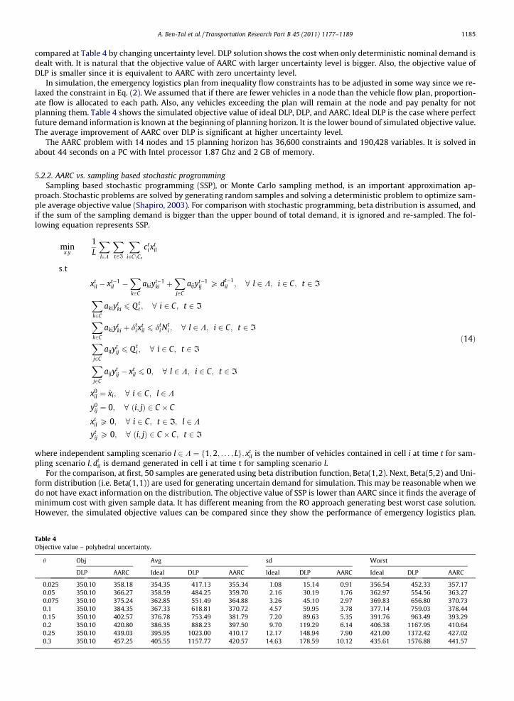
A. Ben-Tal et al. / Transportation Research Part B 45 (2011) 1177–1189 1185

compared at Table 4 by changing uncertainty level. DLP solution shows the cost when only deterministic nominal demand isdealt with. It is natural that the objective value of AARC with larger uncertainty level is bigger. Also, the objective value ofDLP is smaller since it is equivalent to AARC with zero uncertainty level.

In simulation, the emergency logistics plan from inequality flow constraints has to be adjusted in some way since we re-laxed the constraint in Eq. (2). We assumed that if there are fewer vehicles in a node than the vehicle flow plan, proportion-ate flow is allocated to each path. Also, any vehicles exceeding the plan will remain at the node and pay penalty for notplanning them. Table 4 shows the simulated objective value of ideal DLP, DLP, and AARC. Ideal DLP is the case where perfectfuture demand information is known at the beginning of planning horizon. It is the lower bound of simulated objective value.The average improvement of AARC over DLP is significant at higher uncertainty level.

The AARC problem with 14 nodes and 15 planning horizon has 36,600 constraints and 190,428 variables. It is solved inabout 44 seconds on a PC with Intel processor 1.87 Ghz and 2 GB of memory.

5.2.2. AARC vs. sampling based stochastic programmingSampling based stochastic programming (SSP), or Monte Carlo sampling method, is an important approximation ap-

proach. Stochastic problems are solved by generating random samples and solving a deterministic problem to optimize sam-ple average objective value (Shapiro, 2003). For comparison with stochastic programming, beta distribution is assumed, andif the sum of the sampling demand is bigger than the upper bound of total demand, it is ignored and re-sampled. The fol-lowing equation represents SSP.

Table 4Objectiv

h

0.020.050.070.10.150.20.250.3

minx;y

1L

Xl2K

Xt2I

Xi2CnCs

cti x

til

s:t

xtil � xt�1

il �Xk2C

akiyt�1ki þ

Xj2C

aijyt�1ij P dt�1

il ; 8 l 2 K; i 2 C; t 2 I

Xk2C

akiytki 6 Q t

i ; 8 i 2 C; t 2 I

Xk2C

akiytki þ dt

i xtil 6 dt

i Nti ; 8 l 2 K; i 2 C; t 2 I

Xj2C

aijytij 6 Q t

i ; 8 i 2 C; t 2 I

Xj2C

aijytij � xt

il 6 0; 8 l 2 K; i 2 C; t 2 I

x0il ¼ x̂i; 8 i 2 C; l 2 K

y0ij ¼ 0; 8 ði; jÞ 2 C � C

xtil P 0; 8 i 2 C; t 2 I; l 2 K

ytij P 0; 8 i; jð Þ 2 C � C; t 2 I

ð14Þ

where independent sampling scenario l 2 K ¼ f1;2; . . . ; Lg; xtil is the number of vehicles contained in cell i at time t for sam-

pling scenario l; dtil is demand generated in cell i at time t for sampling scenario l.

For the comparison, at first, 50 samples are generated using beta distribution function, Beta(1,2). Next, Beta(5,2) and Uni-form distribution (i.e. Beta(1,1)) are used for generating uncertain demand for simulation. This may be reasonable when wedo not have exact information on the distribution. The objective value of SSP is lower than AARC since it finds the average ofminimum cost with given sample data. It has different meaning from the RO approach generating best worst case solution.However, the simulated objective values can be compared since they show the performance of emergency logistics plan.

e value – polyhedral uncertainty.

Obj Avg sd Worst

DLP AARC Ideal DLP AARC Ideal DLP AARC Ideal DLP AARC

5 350.10 358.18 354.35 417.13 355.34 1.08 15.14 0.91 356.54 452.33 357.17350.10 366.27 358.59 484.25 359.70 2.16 30.19 1.76 362.97 554.56 363.27

5 350.10 375.24 362.85 551.49 364.88 3.26 45.10 2.97 369.83 656.80 370.73350.10 384.35 367.33 618.81 370.72 4.57 59.95 3.78 377.14 759.03 378.44350.10 402.57 376.78 753.49 381.79 7.20 89.63 5.35 391.76 963.49 393.29350.10 420.80 386.35 888.23 397.50 9.70 119.29 6.14 406.38 1167.95 410.64350.10 439.03 395.95 1023.00 410.17 12.17 148.94 7.90 421.00 1372.42 427.02350.10 457.25 405.55 1157.77 420.57 14.63 178.59 10.12 435.61 1576.88 441.57

Table 5AARC vs. SSP when h changes. (Beta(5, 2), L = 50, M = 100.)

h Obj Avg Gap sd Worst

AARC SSP AARC SSP AARC (%) SSP (%) AARC SSP AARC SSP

0.025 358.18 350.50 355.34 368.84 0.28 4 0.91 9.02 357.17 392.490.05 366.27 350.91 359.70 387.57 0.31 8 1.76 18.04 363.27 434.880.075 375.24 351.31 364.88 406.31 0.56 12 2.97 27.06 370.73 477.270.1 384.35 351.71 370.72 425.04 0.92 16 3.78 36.08 378.44 519.660.15 402.80 352.58 381.79 463.30 1.33 23 5.35 54.30 393.29 605.50.2 420.80 353.82 397.50 501.69 2.89 30 6.14 72.44 410.64 691.370.25 439.03 355.59 410.17 540.09 3.95 36 7.90 90.59 427.02 777.270.3 457.25 357.74 420.57 578.50 3.70 43 10.12 108.72 441.57 863.15

1186 A. Ben-Tal et al. / Transportation Research Part B 45 (2011) 1177–1189

When Beta(5,2) is used for simulation, we can see that AARC is better than SSP in terms of the average of the simulatedobjective value in Table 5. The gap between AARC and the ideal solution is very small even with higher uncertainty, e.g.it is less than 4% when the uncertain level is 30%! In contrast for SSP, the gap is increased drastically. As shown in Table6, the average values of the simulated objective value from AARC and SSP are comparable with the random demand fromBeta(1,1).

Under both demand scenarios, AARC provides more stable and robust solution than SSP in the aspect of standard devia-tion and worst case solution. In all cases,the worst case costs of SSP exceed the worst case value of AARC. Moreover, the AARCsolution guarantees the feasibility and provides a guaranteed upper bound on the optimal cost. The SSP solution does notguarantee neither of the above.

Next, we test and summarize the effect of penalty value on the performance of each approach. Table 7 shows that as thevalue of M changes, AARC always provides more stable and robust solution than SSP in the aspect of standard deviation andworst case solution, and provides an evacuation solution that leads to small gap from the ideal solution and can meet all thedemand.

5.3. Cape may county network example

We select another network from Yazici and Ozbay (2007) to increase the size of the problem. Official evacuation routes ofCape May county, New Jersey are considered in Fig. 4, which is composed of 27 nodes including three origin nodes (1, 2, and3) and one super destination node (27). All data except the uncertain demand set are adopted from Yazici and Ozbay (2007)and listed at Table 8. For departure time distribution function, Eq. (13) is used with a = 1 and b = 6. Also, the penalty cost(M)for unmet demand is set to be 100.

Tables 9 and 10 show similar results as the pervious small example. AARC approach improves the transportation solutioncompared to the deterministic model. Also, we can observe that AARC solution provides better results than SSP in terms ofthe worse case solution as well as solution stability.

Table 6AARC vs. SSP when h changes. (Beta(1, 1), L = 50, M = 100.)

h Obj Avg Gap sd Worst

AARC SSP AARC SSP AARC (%) SSP (%) AARC SSP AARC SSP

0.025 358.18 350.20 350.86 352.51 0.41 0.88 2.16 6.13 356.04 357.970.05 366.27 350.30 350.68 354.93 0.55 1.77 4.15 12.26 361.62 401.840.075 375.24 350.40 350.29 357.34 0.63 2.65 6.39 18.40 367.70 427.710.1 384.35 350.50 360.15 359.75 3.66 3.54 7.12 24.53 377.49 453.590.15 402.80 350.74 362.09 364.78 4.61 5.38 10.39 36.99 389.53 505.900.2 420.80 351.34 364.82 370.16 5.75 7.30 14.43 48.78 403.76 560.140.25 439.03 352.80 376.34 375.96 9.37 9.26 15.80 60.93 419.08 618.250.3 457.25 354.63 380.24 381.92 10.71 11.20 20.33 73.06 433.76 677.22

Table 7AARC vs. SSP when M changes. (Beta(5, 2), L = 50, h = 0.1.)

obj avg gap sd worst

M AARC SSP AARC SSP AARC (%) SSP (%) AARC SSP AARC SSP

25 384.35 345.04 370.48 435.43 0.86 18.54 3.91 19.88 379.35 474.4650 384.35 347.63 370.27 474.35 0.80 29.17 4.22 31.82 379.13 539.2875 384.35 349.46 371.06 470.81 1.02 28.18 3.87 36.19 379.61 552.61

100 384.35 350.50 373.69 430.37 1.73 17.16 3.34 37.03 380.42 524.02

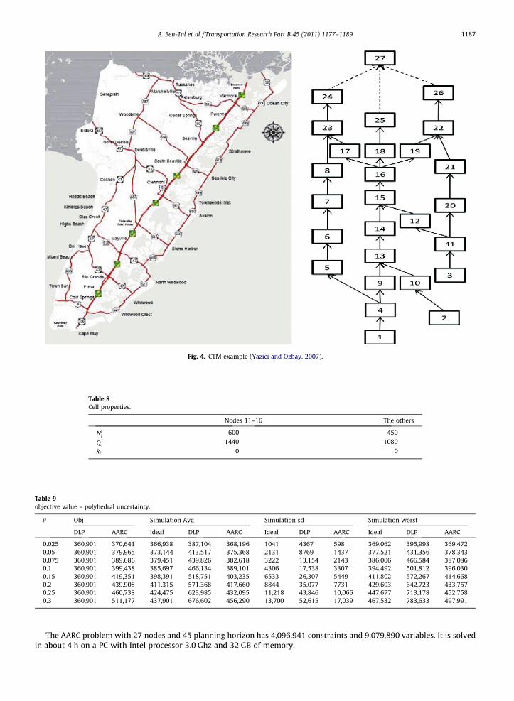
Fig. 4. CTM example (Yazici and Ozbay, 2007).

Table 8Cell properties.

Nodes 11–16 The others

Nti

600 450

Qti

1440 1080

x̂i 0 0

Table 9objective value – polyhedral uncertainty.

h Obj Simulation Avg Simulation sd Simulation worst

DLP AARC Ideal DLP AARC Ideal DLP AARC Ideal DLP AARC

0.025 360,901 370,641 366,938 387,104 368,196 1041 4367 598 369,062 395,998 369,4720.05 360,901 379,965 373,144 413,517 375,368 2131 8769 1437 377,521 431,356 378,3430.075 360,901 389,686 379,451 439,826 382,618 3222 13,154 2143 386,006 466,584 387,0860.1 360,901 399,438 385,697 466,134 389,101 4306 17,538 3307 394,492 501,812 396,0300.15 360,901 419,351 398,391 518,751 403,235 6533 26,307 5449 411,802 572,267 414,6680.2 360,901 439,908 411,315 571,368 417,660 8844 35,077 7731 429,603 642,723 433,7570.25 360,901 460,738 424,475 623,985 432,095 11,218 43,846 10,066 447,677 713,178 452,7580.3 360,901 511,177 437,901 676,602 456,290 13,700 52,615 17,039 467,532 783,633 497,991

A. Ben-Tal et al. / Transportation Research Part B 45 (2011) 1177–1189 1187

The AARC problem with 27 nodes and 45 planning horizon has 4,096,941 constraints and 9,079,890 variables. It is solvedin about 4 h on a PC with Intel processor 3.0 Ghz and 32 GB of memory.

Table 10AARC vs. SSP when h changes. (Beta(5, 2), L = 50, M = 100.)

h Obj Avg Gap sd Worst

AARC SSP AARC SSP AARC (%) SSP (%) AARC SSP AARC SSP

0.025 370,641 356,996 368,196 387,661 0.34 6 598 4363 369,472 396,5620.05 379,965 353,143 375,368 414,563 0.60 11 1437 8761 378,343 432,4360.075 389,686 349,344 382,618 441,409 0.84 16 2143 13,141 387,086 468,2180.1 399,438 345,584 389,101 468,254 0.88 21 3307 17,522 396,030 503,9990.15 419,351 338,247 403,235 521,959 1.22 31 5449 26,282 414,668 575,5780.2 439,908 331,121 417,660 575,665 1.54 40 7731 35,043 433,757 647,1510.25 460,738 324,304 432,095 629,294 1.79 48 10,066 43,805 452,758 718,6510.3 511,177 317,763 456,290 682,927 4.20 56 17,039 52,565 497,991 709,139

1188 A. Ben-Tal et al. / Transportation Research Part B 45 (2011) 1177–1189

6. Conclusion and future work

This paper applied the RO methodology to the CTM based SO-DTA model under demand uncertainty. In particular, AARCwas formulated for dealing with a multi-period transportation problem to find an robust and uncertainty immunized solu-tion, which is especially important in an emergency logistics problem. Two S-shaped curves with upper and lower boundwas introduced by considering uncertainty sets, which are appropriate for modeling uncertain demand. With the linear deci-sion rule for an approximated solution and the appropriate reformulation technique, AARC becomes a linear programmingproblem and hence computationally tractable. The objective value obtained is guaranteed upper bound within a prescribeduncertainty set. Although the AARC solution does not guarantee optimality, we find that the AARC approach leads to highquality solutions compared to the deterministic problem and the sampling based stochastic problem.

However, we do not argue that AARC approach always outperforms the stochastic programming. The proposed AARCmethod is favorable when either reliable information on probability distribution of uncertain parameter is not availableor decision makers want to find a strongly guaranteed performance without facing infeasible solution even in extreme case.In those cases, RO can outperform the traditional stochastic programming approach. Also, the purpose of RO is quite differentfrom sensitivity analysis with variation of parameters. RO finds uncertainty immunized solution for pre-described uncer-tainty set, while sensitivity analysis is a post-optimization tool to test the stability or perturbation of optimal solution(Ben-Tal and Nemirovski, 2000).

Our work has focused on the CTM based SO-DTA problem by using affine control rule for uncertain demand. The reasonfor using the linear decision rule is to derive computational tractable problem. However, theoretically, we do not know howthe approximation makes the robust solution be deviated from the optimal solution. The approximation approach is usedbased on the belief that it is important to provide a solvable problem in emergency logistics field (Shapiro and Nemirovski(2005), Remark 2). The scope of future work could be extended to consider control beyond linear decision rule and to explorelarge scale examples. Moreover, robust optimization approach can be applied to different uncertainty sources (e.g. capacityuncertainty or cost uncertainty) and alternative transportation problems like dynamic network design.

There are other issues raised from this paper. One of these issues is that LP based CTM model allows vehicle holding,which may be unrealistic. RO approach can be applied to alternative deterministic mathematical formulations (e.g. Nie(2010)) to overcome this issue. Extension to considering unbounded uncertainty set with globalized robust optimization(Ben-Tal et al., 2006) is another interesting research direction.

Acknowledgment

This work was partially supported by the grant awards CMMI-0824640 and CMMI-0900040 from the National ScienceFoundation and the Marcus – Technion/PSU Partnership Program.

References

Atamturk, A., Zhang, M., 2007. Two-stage robust network flow and design under demand uncertainty. Operations Research – Baltimore 55 (4), 662–673.Ben-Tal, A., Boyd, S., Nemirovski, A., 2006. Extending scope of robust optimization: comprehensive robust counterparts of uncertain problems.

Mathematical Programming 107 (1), 63–89.Ben-Tal, A., El Ghaoui, L., Nemirovski, A., 2009. Robust Optimization. Princeton University Press.Ben-Tal, A., Goryashko, A., Guslitzer, E., Nemirovski, A., 2004. Adjustable robust solutions of uncertain linear programs. Mathematical Programming 99 (2),

351–376.Ben-Tal, A., Nemirovski, A., 1998. Robust convex optimization. Mathematics of Operations Research 23 (4), 769–805.Ben-Tal, A., Nemirovski, A., 1999. Robust solutions of uncertain linear programs. Operations Research Letters 25 (1), 1–14.Ben-Tal, A., Nemirovski, A., 2000. Robust solutions of linear programming problems contaminated with uncertain data. Mathematical Programming 88 (3),

411–424.Ben-Tal, A., Nemirovski, A., 2002. Robust optimization – methodology and applications. Mathematical Programming 92 (3), 453–480.Bertsimas, D., Brown, D.B., Caramanis, C., 2007. Theory and Applications of Robust Optimization. Submitted. users.ece.utexas.edu/cmcaram/pubs/

RobustOptimizationLV.pdf.Bertsimas, D., Perakis, G., 2005. Robust and adaptive optimization: a tractable approach to optimization under uncertainty. NSF/CMMI/OR 0556106.Bertsimas, D., Sim, M., 2003. Robust discrete optimization and network flows. Mathematical Programming 98 (1), 49–71.

A. Ben-Tal et al. / Transportation Research Part B 45 (2011) 1177–1189 1189

Bertsimas, D., Sim, M., 2004. The price of robustness. Operations Research 52 (1), 35–53.Chiu, Y.C., Zheng, H., Villalobos, J., Gautam, B., 2007. Modeling no-notice mass evacuation using a dynamic traffic flow optimization model. IIE Transactions

39 (1), 83–94.Daganzo, C.F., 1993. The cell transmission model. Part I: a simple dynamic representation of highway traffic. Transportation Research B 28 (2), 269–287.Daganzo, C.F., 1995. The cell transmission model, part II: network traffic. Transportation Research Part B 29 (2), 79–93.El Ghaoui, L., Oks, M., Oustry, F., 2003. Worst-case value-at-risk and robust portfolio optimization: a conic programming approach. Operations Research 51

(4), 543–556.El Ghaoui, L., Oustry, F., AitRami, M., 1997. A cone complementarity linearization algorithm for static output-feedback and related problems. IEEE

Transactions on Automatic Control 42 (8), 1171–1176.Erera, A.L., Morales, J.C., Savelsbergh, M., 2009. Robust optimization for empty repositioning problems. Operations Research 57 (2), 468–483.Friesz, T.L., Bernstein, D., 2000. Handbook of transport modelling. Analytical dynamic traffic assignment models. Pergamon. pp. 181–195.Guha-Sapir, D., Debarati, G.S., Hargitt, D., Hoyois, P., Below, R., Brechet, D., 2004. Thirty Years of Natural Disasters 1974–2003: The Numbers. Presses Univ. de

Louvain.Karoonsoontawong, A., Waller, S.T., 2007. Robust dynamic continuous network design problem. Transportation Research Record: Journal of the

Transportation Research Board 2029 (-1), 58–71.Lindell, M.K., 2008. EMBLEM2: an empirically based large scale evacuation time estimate model. Transportation Research Part A 42, 140–154.Lodree Jr., E.J., Taskin, S., 2008. An insurance risk management framework for disaster relief and supply chain disruption inventory planning. Journal of the

Operational Research Society 59 (5), 674–684.Merchant, D.K., Nemhauser, G.L., 1978a. A model and an algorithm for the dynamic traffic assignment problems. Transportation Science 12 (3), 183.Merchant, D.K., Nemhauser, G.L., 1978b. Optimality conditions for a dynamic traffic assignment model. Transportation Science 12 (3), 200.Mudchanatongsuk, S., Ordonez, F., Liu, J., 2008. Robust solutions for network design under transportation cost and demand uncertainty. Journal of the

Operational Research Society 59 (5), 652–662.Mulvey, J.M., Vanderbei, R.J., Zenios, S.A., 1995. Robust optimization of large-scale systems. Operations Research 43 (2), 264–281.Nie, Y., 2010. A Cell-based Merchant–Nemhauser Model for the System Optimum Dynamic Traffic Assignment Problem. Transportation Research Board 89th

Annual Meeting.Ordóñez, F., Zhao, J., 2007. Robust capacity expansion of network flows. Networks 50 (2), 136–145.Ozdamar, L., Ekinci, E., Kucukyazici, B., 2004. Emergency logistics planning in natural disasters. Annals of Operations Research 129 (1), 217–245.Peeta, S., Zhou, C., 1999. Robustness of the off-line a priori stochastic dynamic traffic assignment solution for on-line operations. Transportation Research

Part C 7 (5), 281–303.Peeta, S., Ziliaskopoulos, A.K., 2001. Foundations of dynamic traffic assignment: the past, the present and the future. Networks and Spatial Economics 1 (3),

233–265.Radwan, A.E., Hobeika, A.G., Sivasailam, D., 1985. A computer simulation model for rural network evacuation under natural disasters. ITE Journal 55 (9), 25–

30.Shapiro, A., 2003. Monte Carlo sampling methods. Handbooks in Operations Research and Management Science 10, 353–426.Shapiro, A., Nemirovski, A., 2005. On Complexity of Stochastic Programming Problems. Springer.Sheu, J.B., 2007. An emergency logistics distribution approach for quick response to urgent relief demand in disasters. Transportation Research Part E 43 (6),

687–709.Tuydes, H., 2005. Network Traffic Management under Disaster Conditions. Ph.D. Thesis, Northwestern University, Evanston, IL.Ukkusuri, S.V., Waller, S.T., 2008. Linear programming models for the user and system optimal dynamic network design problem: formulations,

comparisons and extensions. Networks and Spatial Economics 8 (4), 383–406.Waller, S.T., Schofer, J.L., Ziliaskopoulos, A.K., 2001. Evaluation with traffic assignment under demand uncertainty. Transportation Research Record: Journal

of the Transportation Research Board 1771, 69–74.Waller, S.T., Ziliaskopoulos, A.K., 2006. A chance-constrained based stochastic dynamic traffic assignment model: analysis, formulation and solution

algorithms. Transportation Research Part C 14 (6), 418–427.Xie, C., Lin, D.Y., Travis Waller, S., 2010. A dynamic evacuation network optimization problem with lane reversal and crossing elimination strategies.

Transportation Research Part E 46 (3), 295–316.Yazici, M.A., Ozbay, K., 2007. Impact of probabilistic road capacity constraints on the spatial distribution of hurricane evacuation shelter capacities.

Transportation Research Record: Journal of the Transportation Research Board 2022, 55–62.Yin, Y., Lawphongpanich, S., Lou, Y., 2008. Estimating investment requirement for maintaining and improving highway systems. Transportation Research

Part C 16 (2), 199–211.Yin, Y., Madanat, S.M., Lu, X.Y., 2009. Robust improvement schemes for road networks under demand uncertainty. European Journal of Operational Research

198 (2), 470–479.Ziliaskopoulos, A.K., 2000. A linear programming model for the single destination system optimum dynamic traffic assignment problem. Transportation

Science 34 (1), 37–49.