1 sace stage 1 mathematics statistics linking mathematics with relevant teaching and learning...
TRANSCRIPT
1
SACE Stage 1 Mathematics STATISTICS
LINKING MATHEMATICS WITH RELEVANT TEACHING AND LEARNING PRACTICES IN
THE SENIOR YEARS
Session 1

2
Statistical thinking will one day be as necessary a qualification for efficient citizenship as the
ability to read and write.
--H.G. Wells

3
What is Statistics?
Statistics is the art of solving problems or answering questions that require the collection and analysis of data.

4
What are these workshops?
These workshops present a small number of investigations and activities using statistical methods prescribed in the syllabus.
The purpose is to illustrate the motivation and development of statistical reasoning through its application in problem solving.
5
What they are not
These workshops are not a refresher course on elementary statistics. It is assumed that teachers can access
basic knowledge of the necessary techniques.
There is no discussion of formulas. There are few example calculations. There are no step by step computer or
calculator instruction.
6
What they are not
However, the data are available separately and participants are encouraged to reproduce the calculations between the sessions and experiment with their own analysis.
Some source material is also provided.

7
What they are not
They do not exhaustively cover the syllabus.
It is again assumed that the participants will be able make themselves familiar with this material.

8
What they are not
They are not a practice run for classroom teaching.
They are not detailed lesson plans. In contrast to the classroom, the
routine technical aspects of the subject are not addressed.
Those aspects will, of course, occupy a significant amount of classroom time.
9
Outcomes
At the end of the sessions, it is anticipated the participants will come away with: An appreciation of the elegance and
power of statistical ideas. An appreciation of the role of data
analytic investigation as a vehicle for the development of statistical reasoning and methods.

10
Outcomes
At the end of the sessions, it is anticipated the participants will come away with: A better understanding of what makes
an appropriate investigation. The confidence to implement teaching
programs based on the problem solving approach.

11
Problems to investigate
The Road Accident problem.
The Titanic question.

12
Entering the problem zone
Improving our accident record.
Focus on the recognition of students
prior knowledge.
Video presentation and so on.
13
The road traffic problem
It is widely known that stopping distance of a vehicle increases dramatically with speed.
This can be checked using high school level physics and has been proved experimentally.
For this reason we can be sure that excessive speed increases the risk of accident.
The question of interest is:
By how much?

14
The road traffic problem
If speed is an important factor in a significant number of accidents then there is justification for increased spending on: Driver education. Advertising campaigns. Policing speed laws.
It also justifies the use of speed cameras as life savers rather than revenue raisers.
15
The road traffic problem
If speed is not an important factor then spending could be directed to:
Better roads. Combating drink driving. Vehicle inspections.

16
The Research Question
Were cars involved in serious crashes travelling faster than
other cars?

17
What might we do to answer this question?
Groups suggest an appropriate way to investigate the road accident
problem.

18
The Study
Serious crashes that occurred on rural roads in a 150 km radius of Adelaide were studied.
Alcohol was determined not to be a factor.
The vehicles were travelling at ‘free speed’.

19
Free Speed
Free speed means that the vehicles were travelling without obstruction: They were not trying to overtake another
vehicle. They were not trying to enter a road or
merge with traffic. If they were at an intersection, they had
right of way.

20
Accident Vehicle Speeds
For each ‘free speed’ crash the researchers: Attended the accident scene.
Obtained measurements of tyre marks and point of impact etc.
Used computerized accident reconstruction techniques to estimate the speed of the accident vehicle at the time of the crash.
21
Control Vehicles
For each ‘free speed’ crash the researchers: Returned to the crash scene some days
after the accident.
Chose the same day of week as the actual accident.
Chose the same hour of the day.
Chose a day with similar weather and lighting conditions.

22
Control Vehicles
Identified 10 vehicles travelling at the free speed and measured their speeds using a hand-held radar.
Were careful to conceal themselves from the view of the motorists they were observing.
These vehicles are called the control vehicles.
23
The Accident Data
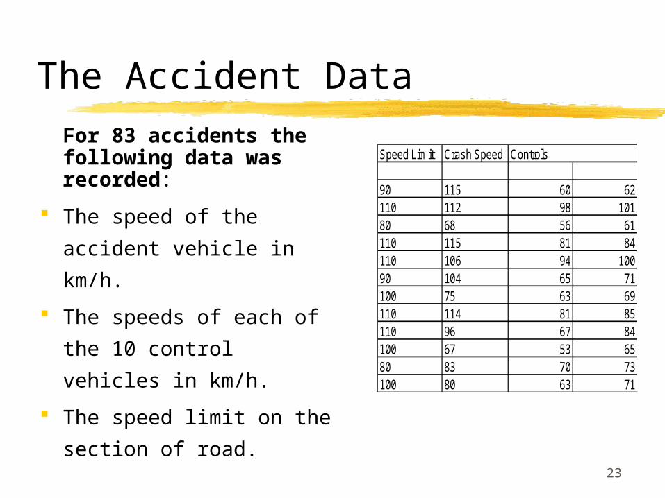
For 83 accidents the following data was recorded:
The speed of the
accident vehicle in km/h.
The speeds of each of
the 10 control vehicles
in km/h.
The speed limit on the
section of road.
Speed Limit Crash Speed
90 115 60 62110 112 98 10180 68 56 61110 115 81 84110 106 94 10090 104 65 71100 75 63 69110 114 81 85110 96 67 84100 67 53 6580 83 70 73100 80 63 71
Controls
24
How might we use this data to answer the question?
Groups consider appropriate ways to investigate the road accident
problem.
25
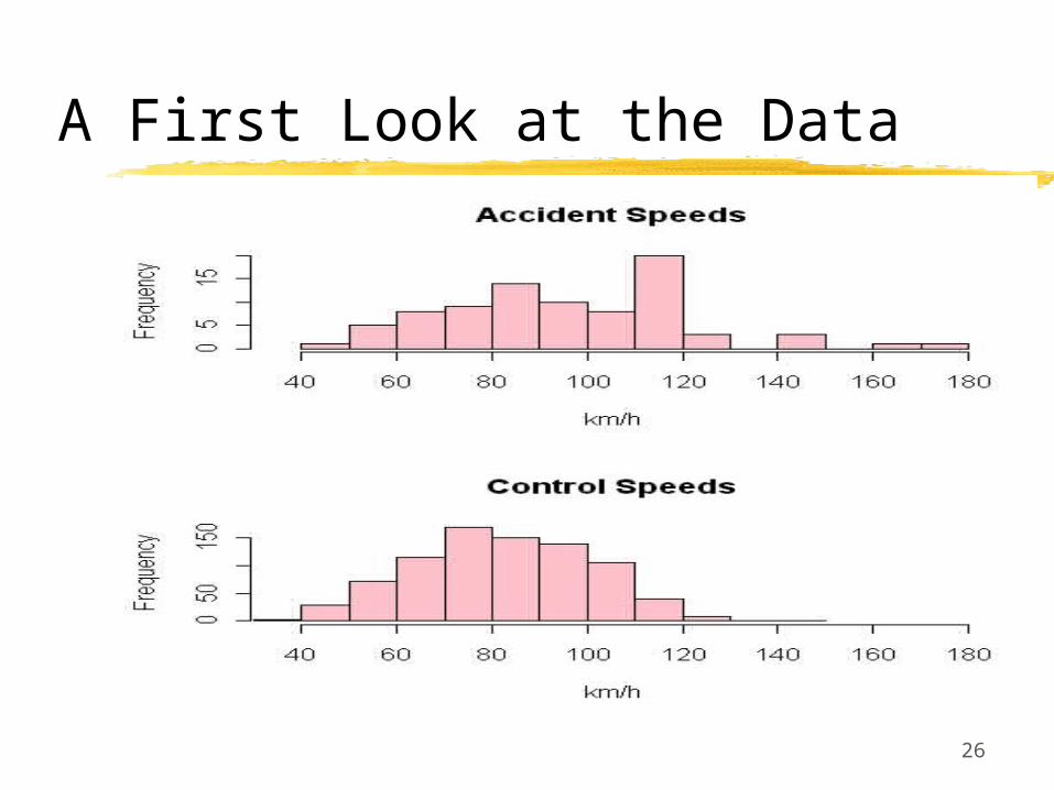
A First Look at the Data
We want to compare the speeds of the 83 accident vehicles to the 830 controls.
Since speed is a quantitative variable, it is appropriate to consider histograms.
We use separate histograms with the same horizontal scale.
26
A First Look at the Data

27
Summary Statistics
Mean Standard Deviation
Accidents
95.7 24.8
Controls 82.6 18.2LQ Median UQ
Accidents
78.5 94.0 112.0
Controls 70.0 82.0 97.0

28
First Conclusions
On average the accident vehicles were travelling 13.1kmk/h faster than the control vehicles.
A small number of the accidents were travelling very fast. (five were going above 140km/hour)
No control vehicles were recorded above 140km/hour.
The accident vehicles had also a peak at 110-119 km/hour.
No such peak was present in the control speeds.

29
The 110-119 km/h Peak
Explanation 1
The researchers were biased toward guessing
near the speed limit when the reconstruction was
difficult. The researchers were sure that this was
not the case.
Explanation 2The drivers misunderstood the “no limit” sign to mean 110km/h instead of 100km/h.

30
Investigating the Peak
Explanation 2 can be investigated by tabulating the speed limits for these vehicles. The majority of these where recorded in 100 km/hour zones
We must compare this to the overall distribution of speed limits
This shows roughly the same percentage amongst all cases, so there is no real evidence for this explanation
110-119 km/hr
Limit 80 90 100 110
CountPercent
14.8%
14.8%
1152.4%
838.1%
All Cases
Limit 80 90 100 110
CountPercent
1720.5%
22.4%
4351.8%
2125.3%

31
Conclusion
Apart from a small number of very high speeds and the unexplained peak between 110-119km/h there appears to be no major differences between the distributions of speed for accidents and controls .

32
Reflections
Have we answered the original research question?
Are we satisfied with this answer?
Groups to consider these points and offer suggestions for further analysis.

33
Entering a new problem zone
An historic adventure.
Focus on the recognition of students prior
knowledge.
Video presentation and so on.

34
Titanic Study
The tragic maiden voyage of the Titanic has captured the interest of many people and it is now our turn to investigate some of the issues related to the voyage.
The question of interest is:
Did all passengers on the Titanic have an equal chance of surviving?

35
Consider the question
Groups to discuss how they might investigate the question.
36
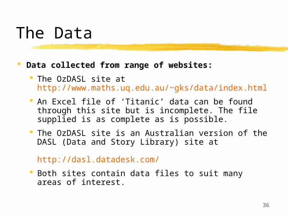
The Data
Data collected from range of websites:
The OzDASL site at http://www.maths.uq.edu.au/~gks/data/index.html
An Excel file of ‘Titanic’ data can be found through this site but is incomplete. The file supplied is as complete as is possible.
The OzDASL site is an Australian version of the DASL (Data and Story Library) site at http://dasl.datadesk.com/
Both sites contain data files to suit many areas of interest.
37
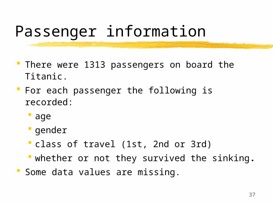
Passenger information
There were 1313 passengers on board the Titanic.
For each passenger the following is recorded: age gender class of travel (1st, 2nd or 3rd) whether or not they survived the sinking.
Some data values are missing.
38
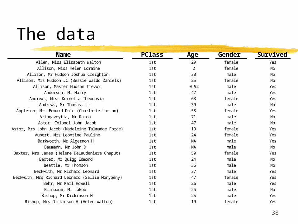
The dataName PClass Age Gender Survived
Allen, Miss Elisabeth Walton 1st 29 female YesAllison, Miss Helen Loraine 1st 2 female No
Allison, Mr Hudson Joshua Creighton 1st 30 male NoAllison, Mrs Hudson JC (Bessie Waldo Daniels) 1st 25 female No
Allison, Master Hudson Trevor 1st 0.92 male YesAnderson, Mr Harry 1st 47 male Yes
Andrews, Miss Kornelia Theodosia 1st 63 female YesAndrews, Mr Thomas, jr 1st 39 male No
Appleton, Mrs Edward Dale (Charlotte Lamson) 1st 58 female YesArtagaveytia, Mr Ramon 1st 71 male No
Astor, Colonel John Jacob 1st 47 male NoAstor, Mrs John Jacob (Madeleine Talmadge Force) 1st 19 female Yes
Aubert, Mrs Leontine Pauline 1st 24 female YesBarkworth, Mr Algernon H 1st NA male Yes
Baumann, Mr John D 1st NA male NoBaxter, Mrs James (Helene DeLaudeniere Chaput) 1st 50 female Yes
Baxter, Mr Quigg Edmond 1st 24 male NoBeattie, Mr Thomson 1st 36 male No
Beckwith, Mr Richard Leonard 1st 37 male YesBeckwith, Mrs Richard Leonard (Sallie Monypeny) 1st 47 female Yes
Behr, Mr Karl Howell 1st 26 male YesBirnbaum, Mr Jakob 1st 25 male No
Bishop, Mr Dickinson H 1st 25 male YesBishop, Mrs Dickinson H (Helen Walton) 1st 19 female Yes

39
How might the data be analysed?
Groups to discuss how they might proceed in order to reach an answer to the
question posed.

40
A first look at the Data
If we want to examine any relationships amongst survivors, then we need to consider the population of passengers on board the Titanic.
Gender, class of travel and survival are categorical variables and the relationship between them can be examined by charts and tables.

41
A summary of the data
Class count %1st 322 24.52nd 280 21.33rd 711 54.2
Gender count %female 462 35.2male 851 64.8
Survival Status count %yes 450 34.3no 863 65.7

42
Comments
From the tabular information we can see that There were more male passengers
than female. The majority of passengers travelled
third class. About one third of the passengers
survived.

43
Comments
While this summary provided a good description of our population, and is an important step, it does not answer our question, more information can be obtained if cross tabulation is used.
44
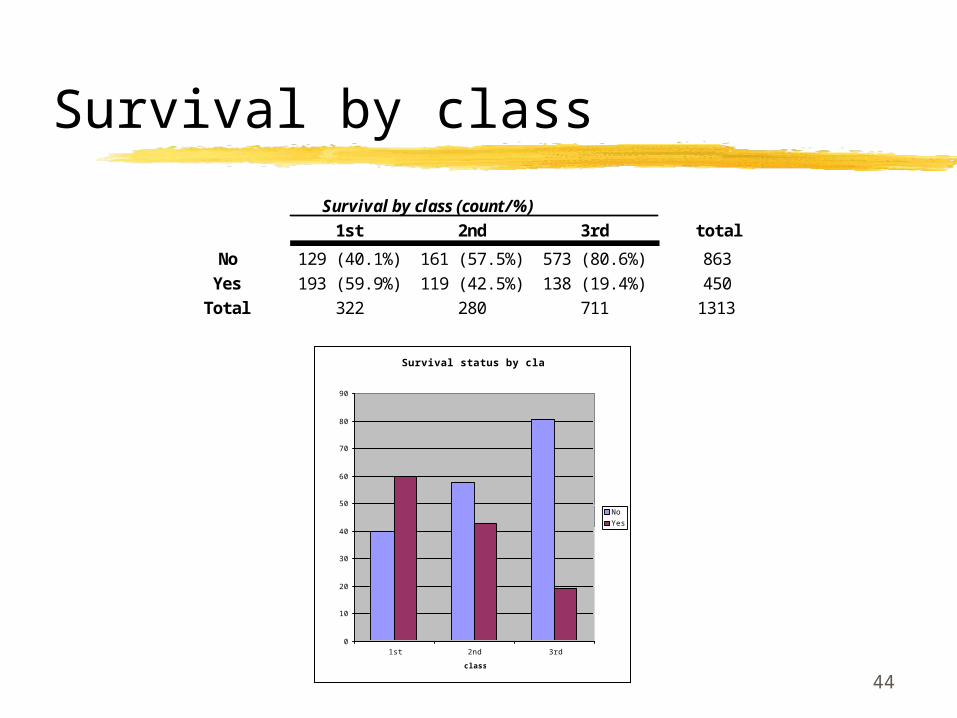
Survival by class
Survival by class (count/%)1st 2nd 3rd total
No 129 (40.1%) 161 (57.5%) 573 (80.6%) 863Yes 193 (59.9%) 119 (42.5%) 138 (19.4%) 450
Total 322 280 711 1313
Survival status by class
0
10
20
30
40
50
60
70
80
90
1st 2nd 3rd
class
perc
en
tag
e
No
Yes
45
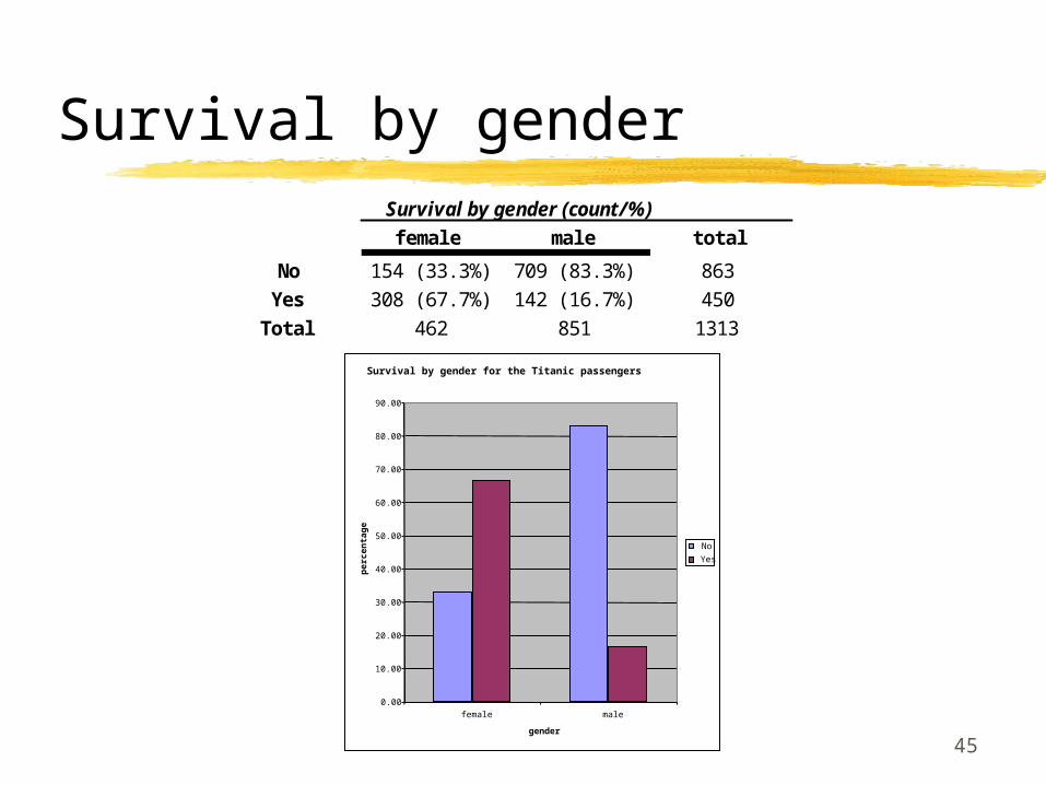
Survival by gender
Survival by gender for the Titanic passengers
0.00
10.00
20.00
30.00
40.00
50.00
60.00
70.00
80.00
90.00
female male
gender
perc
en
tag
e
No
Yes
Survival by gender (count/%)female male total
No 154 (33.3%) 709 (83.3%) 863Yes 308 (67.7%) 142 (16.7%) 450
Total 462 851 1313

46
Observations when two variables are considered
The class with the largest percentage of survivors is first class whereas third class has the smallest percentage of survivors.
The percentage of females surviving is much larger than the percentage of males.

47
Reflections on the observations
Do these observations answer our question?
Are we satisfied with this answer?
Groups reflect and offer suggestions.
48
Gender by class
Offers a way to investigate the gender balance in classes.
Offers a pathway for further analysis.

49
Gender by class
Gender by class (count/%)1st 2nd 3rd total
female 143 (44.4%) 107 (38.2%) 212 (29.8%) 462male 179 (55.6%) 173 (61.8%) 499 (70.2%) 851Total 322 280 711 1313
Gender by class
0.00
10.00
20.00
30.00
40.00
50.00
60.00
70.00
80.00
1st 2nd 3rd
class
perc
en
tag
e
female
male
50
Comments when two variables are considered.
The number of males in third class is more than double the number of females.
Any more comments ?

51
Stratifying still further
Finally we consider the relations amongst the variables when class and survival status are considered separately for males and females.
52
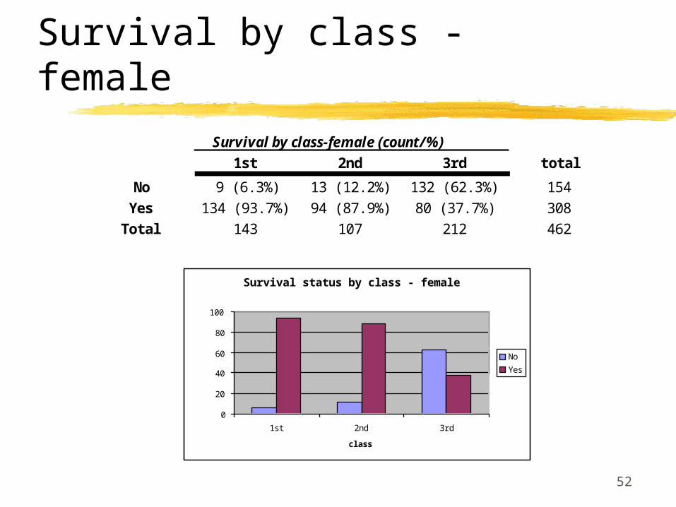
Survival by class - female
Survival by class-female (count/%)1st 2nd 3rd total
No 9 (6.3%) 13 (12.2%) 132 (62.3%) 154Yes 134 (93.7%) 94 (87.9%) 80 (37.7%) 308
Total 143 107 212 462
Survival status by class - female
0
20
40
60
80
100
1st 2nd 3rd
class
perc
enta
ge
No
Yes

53
Survival by class - male
Survival Status by class - male
0
20
40
60
80
100
1st 2nd 3rd
class
perc
enta
ge
No
Yes
Survival by class-male (count/%)1st 2nd 3rd total
No 120 (67.0%) 148 (85.6%) 441 (88.4%) 709Yes 59 (33.0%) 25 (14.5%) 58 (11.6%) 142
Total 179 173 499 851

54
Conclusions using the summary tables
Clearly there are substantial differences so if we return to the question of interest:
“Did all passengers on the Titanic have a fair chance of surviving?”
The tables and charts provide a clear answer - NO!
However, would you rather be a male travelling first class or a female travelling third class?
Is there more worth thinking about?

55
Comparing and contrasting the data structures and tools
Groups compare and contrast the tools and approaches used for the two problems considered thus far.
56
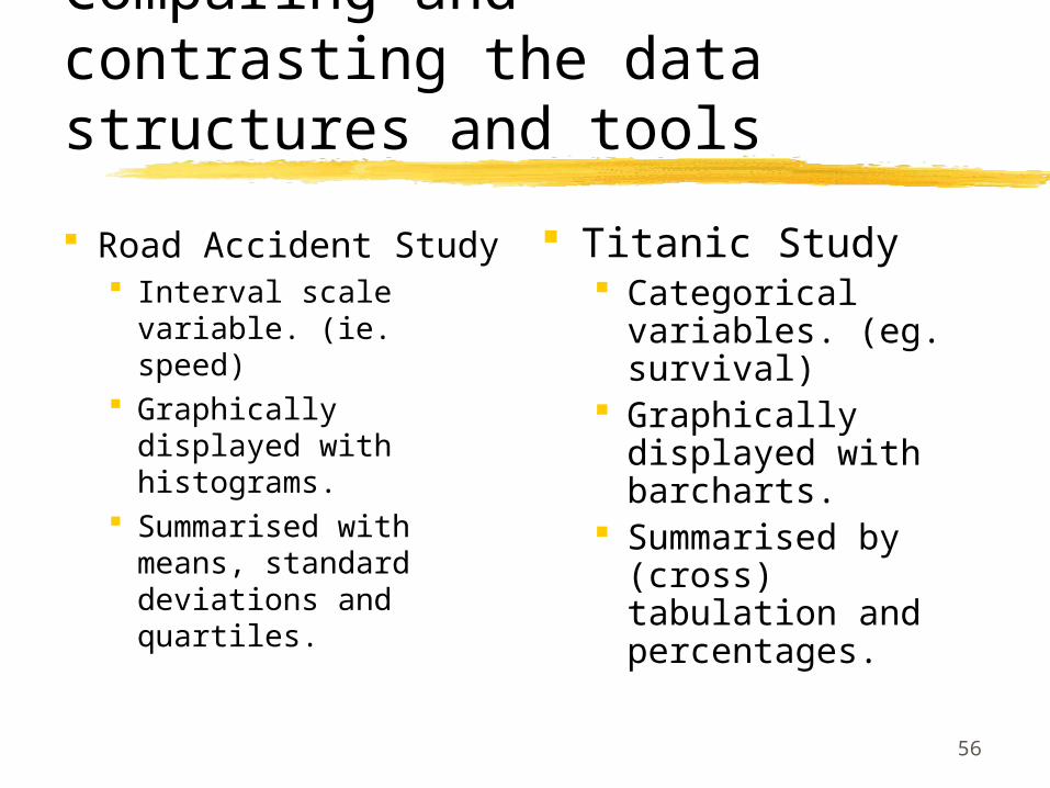
Comparing and contrasting the data structures and tools
Road Accident Study Interval scale
variable. (ie. speed) Graphically
displayed with histograms.
Summarised with means, standard deviations and quartiles.
Titanic Study Categorical
variables. (eg. survival)
Graphically displayed with barcharts.
Summarised by (cross) tabulation and percentages.
57
Choosing the correct graph
If a single variable is to be displayed the key step is to recognise the type of variable
For interval variables we can use histograms,box plots, stem and leaf plots
For categorical variables we can use bar charts.
58
Interval Variables
Histograms Need moderate to large amount of data effective for comparing 2-3 groups
Stem & Leaf Plots Suitable for small - moderate data sets (hand-
production) Effective for comparing 2-3 groups
Boxplots Needs moderate to large amount of data Effective for comparing several groups
59
Categorical Data
Bar Charts Effective for comparing small numbers
of groups and categories Avoid 3-d effects
Pie Charts Not useful for data analysis
Cross-Tabulations Can be very effective for small numbers
of groups and categories

60
Pedagogical reflections
People learn best when initially immersed in a problem similar to one where they will apply the learning.
The problem presented should be interesting and worthwhile, not contrived. Real situations and data are preferable. There must be a question to be
answered. The statistical methods to be learned
must be central in obtaining an answer.

61
Pedagogical reflections
Students should participate in the problem solving process The problems should be such that
students can suggest ways to proceed at key points in the solution’s development
The problems should be structured so that the most intuitive way to proceed leads to the theory that is to be learned

62
Pedagogical reflections
When the solution to the original problem is produced: The problem solving process should be
summarised. The statistical theory and methods should be
summarised and generalised. The key attributes of the problem that make
the methods applicable should be highlighted. Can be reinforced by comparing and
contrasting different problems and techniques.

63
Pedagogical reflections
These workshops are intended to illustrate the role of problem solving in teaching.
This is, of course, only one aspect of teaching.
Many of the micro-issues have not been discussed.

64
Pedagogical reflections
In the classroom a reasonable proportion of time will need to be spent on the micro-issues, such as: Entering and organising data. Obtaining suitable graphs. Obtaining suitable summary statistics. Understanding the formulation of various
statistics.

65
Pedagogical reflections
The role of the problem is to ensure that students see statistics as a coherent methodology for answering questions from data rather than a disparate collection of numerical techniques.

66
An approach to the pedagogy
Start with the general idea of the problem. Use the prior knowledge of the students to focus
in on the problem to be solved. Allow the student to begin solving - until they get
stuck. Leave the problem and do some learning. Go back to the problem at an appropriate time. Cycle in and out of the problem as needed.

67
An approach to the pedagogy
Make the problem visible in the classroom somehow and ensure that when the students learn the more routine material you encourage them to see links from that material to the problem.