1 shortest path calculations in graphs prof. s. m. lee department of computer science
TRANSCRIPT

1
Shortest Path Shortest Path CalculationsCalculations
ininGraphsGraphs
Prof. S. M. LeeDepartment of Computer Science

2
Topic Overview
Review of Graphs
Unweighted Shortest Path Problem
Positive Weighted Shortest Path Problem

3
Review of graphs
A graph represents relationship among items.
A graph consists of a set of vertices and a set of edges that connect the vertices.
G = (V, E)G = (V, E)

4
Review of graphs (cont.) V: the set of vertices (or nodes) E: the set of pairs of edges that
connect the vertices
V2 V3
V0 V1
Vertex
Edge

5
Example:
computing the fastest route through mass transportation
computing the fastest way for routing electronic mail through a network of computers

6
Optimization Problem
Input: X Output: Y subject to: an objective
function f(Y) is optimized in all possible Y's satisfying constraints^^^^^^^^^^^^^ feasible solutions
The greedy method regards an optimization problem as finding a sequence of decisions that optimizes the objective function.

7
Selection Function ------------------ To measure "how promising" each candidate for a decision leads to an optimal solution
Greedy Method ------------- At each stage of decision, choose a candidate which has the largest value of the selection function.

8

9

10
Who discovered the shortest pathWho discovered the shortest path algorithm?algorithm?
• Edsger Wybe Dijkstra was born 1930.• He began programming computers in the early 1950s at the University of Leiden.• Dijkstra has been one of the most forceful proponents of programming as a scientific discipline.• He has made fundamental contributions to the areas of operating systems, including deadlock avoidance; programming languages including the notion of structured programming and algorithm.

11

12

13

14

15

16

17

18

19

20

21
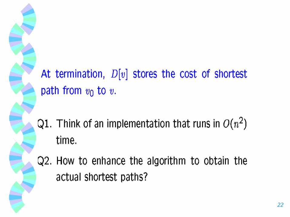
22

23
Traces the Dijkstra’s shortestTraces the Dijkstra’s shortest path algorithmpath algorithm
0 1 2
3 4
8 2
1
9
4 3
2
1
7
A weighted directed graph

24
Traces the Dijkstra’s shortestTraces the Dijkstra’s shortest path algorithmpath algorithm
0 1 2 3 40
1
2
3
4
8 9 4
1
2 3
2 7
1
(Adjacency matrix)

25
Traces the Dijkstra’s shortestTraces the Dijkstra’s shortest path algorithmpath algorithm
Step1: S initially contains vertex 0, and W is initially the first row of the
graph’s adjacency matrix, shown in the previous slides.

26
Traces the Dijkstra’s shortestTraces the Dijkstra’s shortest path algorithmpath algorithmStep 2: W[4] = 4 is the smallest value in W,
ignoring W[0] because 0 is in S. Thus, v = 4, so add 4 to S. For vertices not in S, that is, for u = 1, 2, and 3, check whether it is shorter to
go from 0 to 4 and then along an edge to u instead of directly from 0 to u along an edge. For vertices 1 and 3, it is not shorter to include vertex 4
in the path.

27
Traces the Dijkstra’s shortestTraces the Dijkstra’s shortest path algorithmpath algorithm
Step 2 (continue): However, for vertex 2 notice that W[2] = > W[4] +
A[4][2] = 4 + 1 = 5. Therefore, replace W[2] with 5. You can also verify this conclusion by examining the graph directly.

28
Traces the Dijkstra’s shortestTraces the Dijkstra’s shortest path algorithmpath algorithm
Step2: The path 0 - 4 - 2 is shorter than 0 - 2.
0 2
4
4 1

29
Traces the Dijkstra’s shortestTraces the Dijkstra’s shortest path algorithmpath algorithmStep 3: W[2] = 5 is the smallest value in W,
ignoring W[0] and W[4] because 0 and 4 are in S. Thus, v = 2, so add 2 to S. For vertices not in S, that is for u = 1 and 3, check whether it is shorter to go to u along as edge. Notion that W[1] = 8 > W[2] + A[2][1] = 5 +2 = 7. Therefore, replace W[1] with 7.

30
Traces the Dijkstra’s shortestTraces the Dijkstra’s shortest path algorithmpath algorithm
Step 3: The path 0 - 4 - 2 - 1 is shorter that 0 - 1.
0 12
4
8 2
4 1

31
Traces the Dijkstra’s shortestTraces the Dijkstra’s shortest path algorithmpath algorithm
Step 3 (continue): The path 0 - 4 - 2 - 3 is shorter than 0 - 3.
0
3 4
243
19

32
Traces the Dijkstra’s shortestTraces the Dijkstra’s shortest path algorithmpath algorithm
Step 4: W[1] = 7 is the smallest value in W, ignoring W[0], W[2], and W[4] because 0, 2 and 4 are in S. Thus, v = 1, so add 1 to S. For vertex 3, which is the only
vertex not in S, notion that W[3] = 8 < W[1] + A[1][3] = 7 + . Therefore, leave W[3] as it is.
33
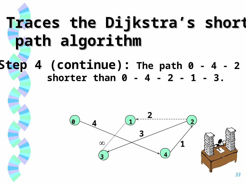
Traces the Dijkstra’s shortestTraces the Dijkstra’s shortest path algorithmpath algorithm
Step 4 (continue): The path 0 - 4 - 2 - 3 is shorter than 0 - 4 - 2 - 1 - 3.
0 1 2
3 4
42
31

34
Traces the Dijkstra’s shortestTraces the Dijkstra’s shortest path algorithmpath algorithm
Step 5 : The only remaining vertex not in S is 3, so add it to S and stop.

35
Traces the Dijkstra’s shortestTraces the Dijkstra’s shortest path algorithmpath algorithmStep V S W[0] W[1] W[2] W[3] W[4]1 - 0 0 8 9 1
2 4 0, 4 0 8 5 9 43 2 0,4,2 0 7 5 8 44 1 0,4,2,1 0 7 5 8 45 3 0,4,2,1,3 0 7 5 8 4
36
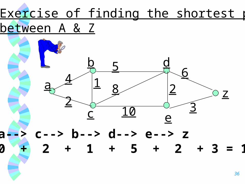
Exercise of finding the shortest pathbetween A & Z
a
b
c
d
e
z4
2
15
8
10
62
3
a--> c--> b--> d--> e--> z0 + 2 + 1 + 5 + 2 + 3 = 13

37
Theory We will use Dijkstra’s algorithm to solve
the weighted shortest path problem.
We can also use the same algorithm to solve the unweighted shortest path problem by considering its edges’ weights as 1.
Under this algorithm, we use breadth-first search to process vertices in layers: the closest to the start are evaluated first.

38
Unweighted Shortest Path Problem To find the shortest path (measured by number of edges)
from a designed vertex S to every vertex.
V2
V5 V6
V4V3
V1V0 • We will use the breadth-first search to process vertices in layers.
• We will use a tool called eyeball to travel from vertex to vertex.
• We will use V2 as the starting vertex S.
Eyeball at V2
initially
S

39
Unweighted Shortest Path Problem
•We define Di be the length of the shortest path from S to i.
So, DS = 0
and we set Di = initially for all i S
If v is the vertex that the eyeball is currently on, then, for all w that are adjacent to v,
we set Dw = Dv + 1 if Dw = Since the eyeball is currently on V2 , we set:
DV0 = 0 + 1 = 1 & DV5 = 0 + 1 = 1
V2
V5 V6
V4V3
V1V0
0
S

40
Unweighted Shortest Path Problem
Then, we move the eyeball to V0 . From V0 , we can find vertices whose shortest path from S is exactly 2, they are V1 and V3 .
V2
V5 V6
V4V3
V1V0
0
1
1
V2
V5 V6
V4V3
V1V0
0
1 2
2
1 S

41
Unweighted Shortest Path Problem
After we have processed all of V0’s adjacent vertices (V1 & V3), we move the eyeball to V5 which has the same distance from vertex S as V0 does.
Since V5 does not have any out-edge, we move the eyeball to V1 whose length is larger than V5 by 1.
V2
V5 V6
V4V3
V1V0
0
1 2
2
1
V2
V5 V6
V4V3
V1V0
0
1 2
32
1 S

42
Unweighted Shortest Path Problem
From V1 , we can find vertices whose shortest path from S is exactly 3, it is V4 . There is also an edge from V1 to V3 . However, we do not change DV3 since V3 had already been processed.
After we have processed all of V1’s adjacent vertices (V4), we move the eyeball to V3 and set DV6 to 3.
V2
V5 V6
V4V3
V1V0
0
1 2
32
1
V2
V5 V6
V4V3
V1V0
0
1 2
32
1 3S
43
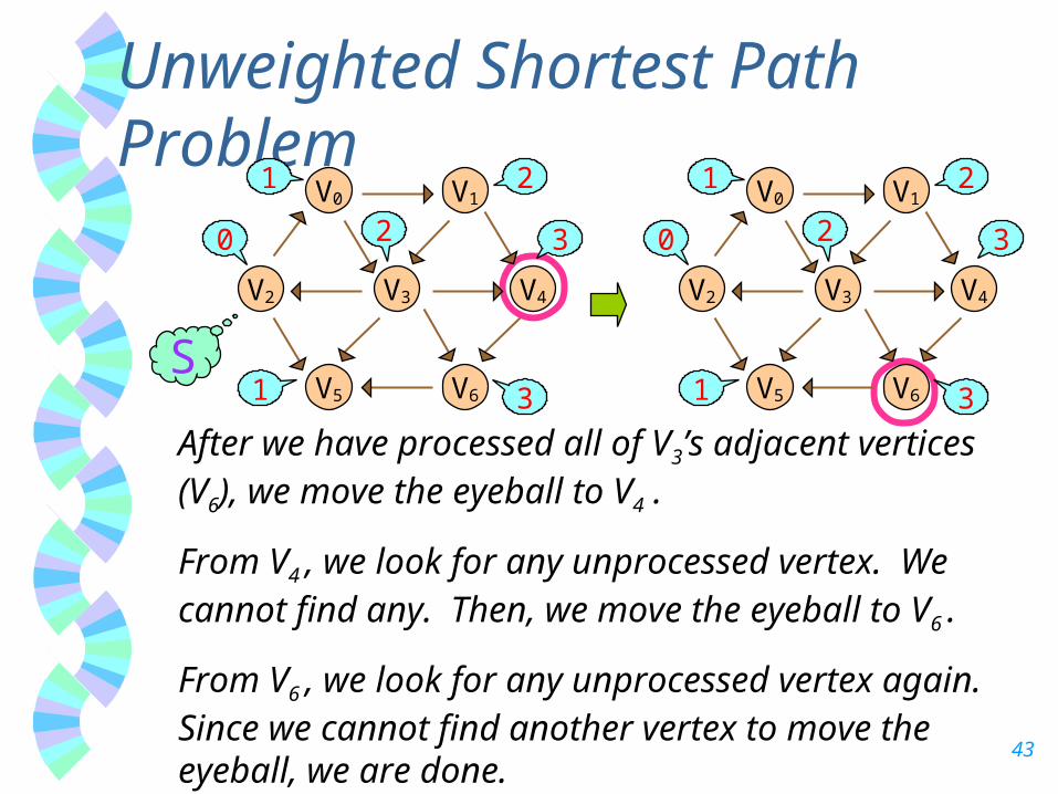
Unweighted Shortest Path Problem
After we have processed all of V3’s adjacent vertices (V6), we move the eyeball to V4 .
From V4 , we look for any unprocessed vertex. We cannot find any. Then, we move the eyeball to V6 .
From V6 , we look for any unprocessed vertex again. Since we cannot find another vertex to move the eyeball, we are done.
V2
V5 V6
V4V3
V1V0
0
1 2
32
1 3
V2
V5 V6
V4V3
V1V0
0
1 2
32
1 3S

44
Positive WeightedShortest Path Problem
First, we start from V0 and consider it as vertex S.
Then, we define Di be the length of the shortest path from S to i. So, DS = 0 and
we set Di = initially for all i S
V2
V5 V6
V4V3
V1
V00
S
4 1
2
310
1
4
2 2
85 6
FrontRearPriorityQueue
Moreover, we use a priority queue to store the vertices needed to be visited next. Every time the Di changes, its vertex will be put into the priority queue.

45
Positive WeightedShortest Path Problem
From V0 , we can find the adjacent vertices V3 and V1
. We put them into the priority queue and update their lengths (Di ) from to 1 and 2 respectively.
Every time Di changes to a smaller number, we put the vertex into the priority queue.
V00
V2
V5 V6
V4V3
V1
2
1
4 1
2
310
1
4
2 2
85 6
V1 V3
FrontRearPriorityQueue
S

46
Positive WeightedShortest Path Problem
Then, we move the eyeball to V3 according to the priority queue. From V3 , we can find the adjacent vertices V4 , V2 , V6 , and V5 . We put them into the priority queue and update their lengths (Di ).
V2
V5 V6
V4V3
V1
2
1
V00
S
4 1
2
310
1
4
2 2
85 6
V00
V2
V5 V6
V4V3
V1
3
2
31
9 5
4 1
2
310
1
4
2 2
85 6
V1 V3
FrontRearPriorityQueue
V5 V2V6 V4 V1
FrontRearPriorityQueue
47
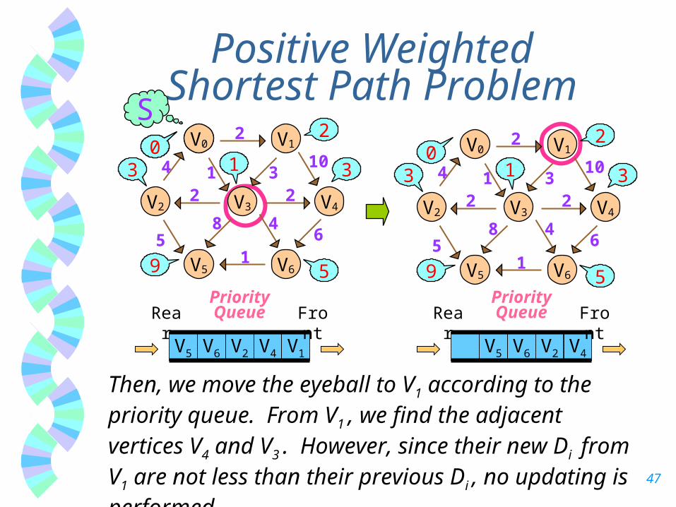
Positive WeightedShortest Path Problem
Then, we move the eyeball to V1 according to the priority queue. From V1 , we find the adjacent vertices V4 and V3 . However, since their new Di from V1 are not less than their previous Di , no updating is performed.
V00
V2
V5 V6
V4V3
V1
3
2
31
9 5
4 1
2
310
1
4
2 2
85 6
V00
SV00
V2
V5 V6
V4V3
V1
3
2
31
9 5
4 1
2
310
1
4
2 2
85 6
V5 V2V6 V4 V1
FrontRearPriorityQueue
V6V5 V2 V4
FrontRearPriorityQueue

48
V6V5 V2 V4
FrontRearPriorityQueue
Positive WeightedShortest Path Problem
After that, we move the eyeball to V4 . From V4 , we find the adjacent vertices V6 . However, since its new Di (9) from V4 is not less than their previous Di (5), no updating is performed.
V00
V2
V5 V6
V4V3
V1
3
2
31
9 5
4 1
2
310
1
4
2 2
85 6
V00
SV00
V2
V5 V6
V4V3
V1
3
2
31
9 5
4 1
2
310
1
4
2 2
85 6
V5 V6 V2
FrontRearPriorityQueue
49
V5 V6 V2
FrontRearPriorityQueue
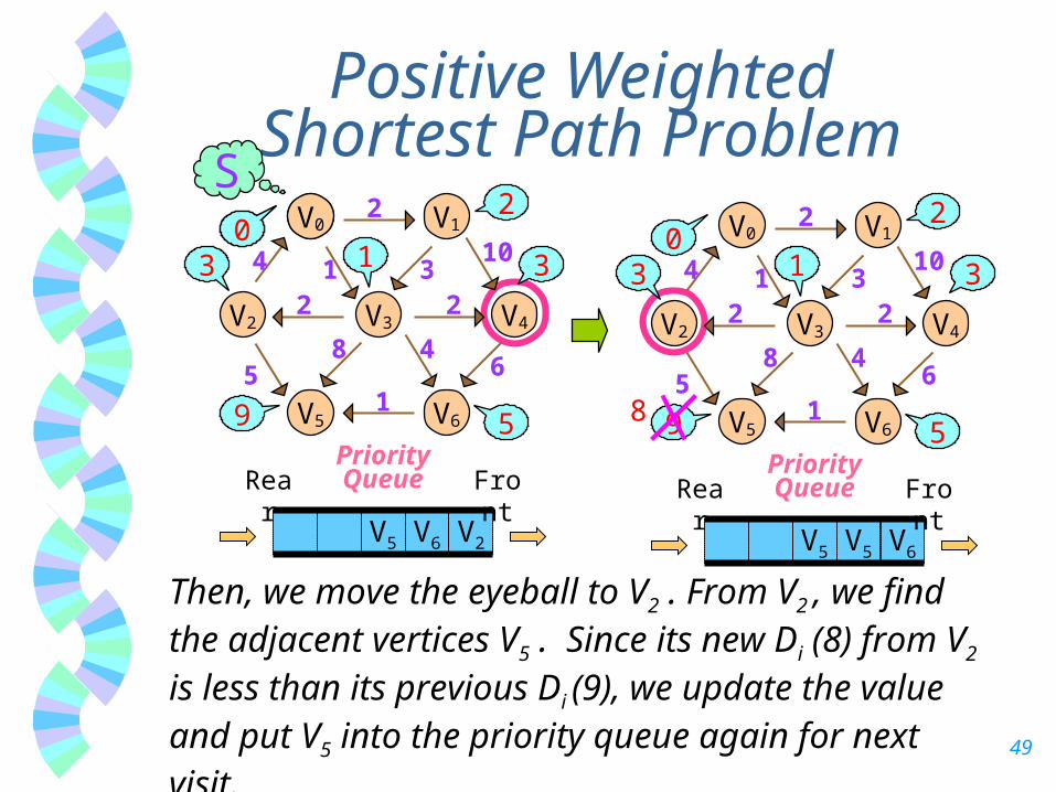
Positive WeightedShortest Path Problem
Then, we move the eyeball to V2 . From V2 , we find the adjacent vertices V5 . Since its new Di (8) from V2 is less than its previous Di (9), we update the value and put V5 into the priority queue again for next visit.
V00
V2
V5 V6
V4V3
V1
3
2
31
9 5
4 1
2
310
1
4
2 2
85 6
V00
S
V5 V5 V6
FrontRearPriorityQueue
V00
V2
V5 V6
V4V3
V1
3
2
31
9 5
4 1
2
310
1
4
2 2
85 6
8

50
V5 V5 V6
FrontRearPriorityQueue
Positive WeightedShortest Path Problem
Then, we move the eyeball to V6 . From V6 , we find the adjacent vertices V5 . Since its new Di (6) from V6 is less than its previous Di (8), we update the value and put V5 into the priority queue again for next visit.
V00
V2
V5 V6
V4V3
V1
3
2
31
9 5
4 1
2
310
1
4
2 2
85 6
8
V00
S
V5 V5 V5
FrontRearPriorityQueue
V00
V2
V5 V6
V4V3
V1
3
2
31
9 5
4 1
2
310
1
4
2 2
85 6
86

51
V5 V5 V5
FrontRearPriorityQueue
Positive WeightedShortest Path Problem
Finally, we move the eyeball to V5 . There is no out-edge in V5 , so we cannot find any adjacent vertices. Therefore, the eyeball is relocated to V5 two more time until the priority queue is cleared. Then, we are done.
V00
V2
V5 V6
V4V3
V1
3
2
31
9 5
4 1
2
310
1
4
2 2
85 6
86
V00
S
FrontRearPriorityQueue
V00
V2
V5 V6
V4V3
V1
3
2
31
9 5
4 1
2
310
1
4
2 2
85 6
86

52

53

54
55

56
57

58

59

60
Various Graph Problems-------------------------
Maximum Network Flow O(e n log n)
Bipartite Matching O(n^{5/2})
Planarity O(n)
Graph Isomorphism
Graph Coloring
Maximum Clique
Maximum Independent Set