1 statistical terminology and descriptive...

QMIN (2006-02-07) Statistical Terminology - 1.1

1 Statistical Terminology and Descriptive StatisticsLike many sciences, statistics involves jargon. Learning the terminology can be

challenging because the definition of one term often assumes some working knowledgeof other terms, not all of which can be defined at the same time. For example, to explaina boxplot, one must already know the meaning of a mean, median, a quartile, and anoutlier.

In this chapter, we introduce some of the key terms in statistics, and in the processoverview what is termed descriptive statistics. In some cases, only the definitions aregiven, leaving a more complete explanation of the phenomena to a later section of thetext. This approach can create some confusion for the student, but we feel that it is bestto obtain at least a partial appreciation for the language first instead of reiterating aconcept and then providing it with a different name.

After developing some mathematical tools, we reconsider the data set and thenbriefly discuss the concept of a distribution. We then define of parametric andnonparametric statistics and give a brief introduction to the two major phases of statisticalprocesses—estimation and inference. We end by explaining descriptive statistics.

1.1 Statistical and Mathematical ToolsWith the two exceptions notes below, all the mathematics needed to understand

most of this text may be found in a high school or lower college division algebra course.A rudimentary knowledge of calculus is helpful to understand fully some of theadvanced—but optional—sections. The two exceptions to this rule are the summationoperator and the product operator.

1.1.1 The Summation OperatorThe summation operation is designated by a symbol resembling the Greek upper

case letter sigma (Σ). The generic form of the summation operator is

€

algebraic expressionalgebraic index= start value

end value

∑ ,

and the operator means take the sum of the results of the algebraic expression that followsit. For example,

€

Xi = X1 +i=1

4

∑ X2 + X3 + X4

and

€

(Xi − X ) = (X2 − X ) +i= 2

4

∑ (X3 − X ) + (X4 − X ) .

Be careful of mathematical operators in summation notation. Operators placedbefore the summation sign denote that the summation occurs first and then themathematical operation is performed. For example,

€

log Yi = log(Y1 +Y2 +Y3)i=1

3

∑ .


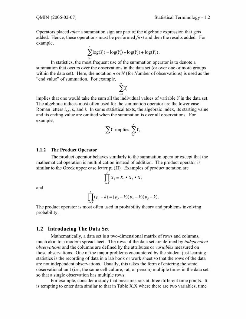
Operators placed after a summation sign are part of the algebraic expression that getsadded. Hence, these operations must be performed first and then the results added. Forexample,

€

log(Yi) = log(Y1) +i=1

3

∑ log(Y2) + log(Y3).

In statistics, the most frequent use of the summation operator is to denote asummation that occurs over the observations in the data set (or over one or more groupswithin the data set). Here, the notation n or N (for Number of observations) is used as the“end value” of summation. For example,

€

Yii=1

N

∑implies that one would take the sum all the individual values of variable Y in the data set.The algebraic indices most often used for the summation operator are the lower caseRoman letters i, j, k, and l. In some statistical texts, the algebraic index, its starting valueand its ending value are omitted when the summation is over all observations. Forexample,

€

Y∑ implies

€

Yii=1

N

∑ .

1.1.2 The Product OperatorThe product operator behaves similarly to the summation operator except that the

mathematical operation is multiplication instead of addition. The product operator issimilar to the Greek upper case letter pi (Π). Examples of product notation are

€

Xi = X1 • X2 • X3i=1

3

∏and

€

(pi − k)i= 3

5

∏ = (p3 − k)(p4 − k)(p5 − k) .

The product operator is most often used in probability theory and problems involvingprobability.

1.2 Introducing The Data SetMathematically, a data set is a two-dimensional matrix of rows and columns,

much akin to a modern spreadsheet. The rows of the data set are defined by independentobservations and the columns are defined by the attributes or variables measured onthose observations. One of the major problems encountered by the student just learningstatistics is the recording of data in a lab book or work sheet so that the rows of the dataare not independent observations. Usually, this takes the form of entering the sameobservational unit (i.e., the same cell culture, rat, or person) multiple times in the data setso that a single observation has multiple rows.

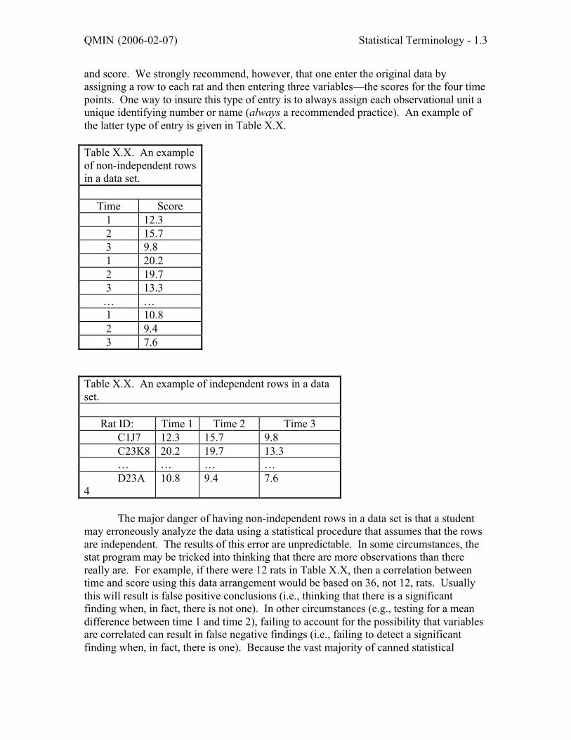
For example, consider a study that measures rats at three different time points. Itis tempting to enter data similar to that in Table X.X where there are two variables, time


and score. We strongly recommend, however, that one enter the original data byassigning a row to each rat and then entering three variables—the scores for the four timepoints. One way to insure this type of entry is to always assign each observational unit aunique identifying number or name (always a recommended practice). An example ofthe latter type of entry is given in Table X.X.

Table X.X. An exampleof non-independent rowsin a data set.

Time Score1 12.32 15.73 9.81 20.22 19.73 13.3

… …1 10.82 9.43 7.6

Table X.X. An example of independent rows in a dataset.

Rat ID: Time 1 Time 2 Time 3C1J7 12.3 15.7 9.8C23K8 20.2 19.7 13.3… … … …D23A

410.8 9.4 7.6

The major danger of having non-independent rows in a data set is that a studentmay erroneously analyze the data using a statistical procedure that assumes that the rowsare independent. The results of this error are unpredictable. In some circumstances, thestat program may be tricked into thinking that there are more observations than therereally are. For example, if there were 12 rats in Table X.X, then a correlation betweentime and score using this data arrangement would be based on 36, not 12, rats. Usuallythis will result is false positive conclusions (i.e., thinking that there is a significantfinding when, in fact, there is not one). In other circumstances (e.g., testing for a meandifference between time 1 and time 2), failing to account for the possibility that variablesare correlated can result in false negative findings (i.e., failing to detect a significantfinding when, in fact, there is one). Because the vast majority of canned statistical


procedures make the assumption of independent rows, errors are most easily avoided byensuring that data entry conforms to the rules for Table X.X and not for Table X.X1.

1.2.1 An Example Data SetHere, we present a real data set that will be used in other sections of this chapter

to illustrate statistical terminology and descriptive statistics. Table X.X gives a listing ofdata based on Bowers et al. (19xx) that examined the effect of the protein kinase C-gamma gene on anxiety in mice. These mice in this study all have the same geneticbackground but differ in genotypes for the PKC-g gene. Transgenic methods were usedto knock out the gene and then cross breeding used to produce three genotypes—thosecompletely deficient in PKC-g (the “--“ genotype in Table 1), the heterozygote with oneknockout allele and one normal allele (the “+-“ genotype), and the homozygote with twonormal alleles (the “++” genotype). The other variable in the data set is called“openarm.” It measures the percent of total time in an elevated plus-maze spent in theopen (versus the closed) arm of the maze. A low percent of time in the open arm isassociated with high levels of anxiety. Note that the actual data set has one and only oneobservation per row, giving a matrix of 45 rows and two columns. The data in Table X.Xare organized differently only to save space.

Table X.X

Genotype Openarm Genotype Openarm Genotype Openarm- - 15.8 + - 5.2 + + 10.6- - 16.5 + - 8.7 + + 6.4- - 37.7 + - 0.0 + + 2.7- - 28.7 + - 22.2 + + 11.8- - 5.8 + - 5.5 + + 0.4- - 13.7 + - 8.4 + + 13.9- - 19.2 + - 17.2 + + 0.0- - 2.5 + - 11.9 + + 16.5- - 14.4 + - 7.6 + + 9.2- - 25.7 + - 10.4 + + 14.5- - 26.9 + - 7.7 + + 11.1- - 21.7 + - 13.4 + + 3.5- - 15.2 + - 2.2 + + 8.0- - 26.5 + - 9.5 + + 20.7- - 20.5 + - 0.0 + + 0.0

1 Having said this, we offer a caveat. Some computer procedures (mostly graphical onesbut also a few statistical ones) are most easily used when data are arranged as non-independent observations. In such cases, we recommend entering the data as independentobservations but then creating a temporary data set that rearranges the data for suchprocedures.


Variable openarm is measured on a ratio scale. Because the total testing time wasthe same for each animal, a mouse that spend 20% of the time in the open arm spenttwice as time there than a mouse with a score of 10.0. Because this variable is a percent,it is bounded.

Variable genotype is nominal, but this is not the best way to deal with thisvariable. Once again, ask whether one could present results for the three groups in anyorder. If the answer is “yes,” then the variable can be treated as categorical. Allgeneticists, however, would present results for the heterozygotye (genotype “+-“)between the results for the two homozygotes. Hence, instead of treating genotype ascategorical, it would be better to create a new variable that would reflect the ordering ofthe data. There are several ways of doing this—use the ordinal number of 1, 2, and 3 torespectively denote genotypes “- -“, “+ -“ and “++”, create a variable for the number of “-“ alleles, or one for the number of “+” alleles.

1.2.2 The Distribution of ScoresMuch statistical terminology talks of a distribution of scores. We deal with this

topic more fully later in X.X Graphing Data, but here introduce the concept of ahistogram to provide a brief overview of a distribution.

There are two types of distributions. The first is the empirical distribution thatgives a figure and/or summary statistics for the observed data at hand. The second is atheoretical distribution or a mathematical model of the way in which the data areassumed to be distributed in an ideal population. A classic example of a theoreticaldistribution is the normal curve. We will have much more to say about theoreticaldistributions later—we just want to introduce the terminology here.

The easiest way to examine an empirical distribution is through graphicalmethods. Figure X.X illustrates a histogram of the variable openarm in the pkc data. In ahistogram, one groups the data into intervals of equal size. In Figure X.X. there are eightintervals, the midpoint of each being presented in the labels of the horizontal axis. Forexample, the first interval consists of scores between –2.5 to 2.499992 (with a midpoint of0), the second from 2.5 to 7.49999 with a midpoint of 5, and so on.

The vertical axis gives the number of observations with scores that fall into theinterval. For example, in the pkc data, six observations fell into the interval of –2.5 to2.5, seven into the interval between 2.5 and 7.5, and so on. In some computer programs,the vertical axis may also be expressed in terms of the percentage or the proportion ofobservations that fall into an interval.

2 Strictly speaking, a number just less than 2.5.


1.2.2.1 Attributes of DistributionsStatisticians speak of several major attributes of distributions. The first of these is

location, or the score(s) around which the distribution is centered. The second is spreador the variability or diversity of scores around the location. The third is symmetry or theextent to which the right-hand side of a distribution is a mirror image of the left-handside. The fourth is peakedness or the extent to which a distribution, given its spread, isflat versus peaked. We discuss these later under descriptive statistics, but in order tounderstand descriptive stats, it is first necessary to digress into an explanation ofparametric and nonparametric statistics.

1.3 Parametric and Nonparametric Statistics:

1.3.1 Populations, Parameters, Samples, and StatisticsLater, we will provide in-depth treatment of the concept of parametric statistics

and probability theory. In this section, we merely provide definitions that will be usefulin the interim. The branch of statistics known as parametric statistics deals withmathematical equations that apply to a population. The population may be humans,schizophrenics, rats, an inbred strain of mice, or aged nematodes. The equations mayinclude those assumed to represent a distribution of scores (e.g., a normal curve) or thoseused to predict one or more variables from knowledge of other variables (e.g., regression,dealt with in Chapter XX).

A parameter is defined as an unknown in a mathematical equation that applies toa population. For example, the mathematical equation for a normal curve contains twounknowns—the mean of the curve and the standard deviation of the curve. It iscustomary to use Greek letters to denote parameters. The most frequently encounteredparameters and their customary symbols are the mean (µ), the standard deviation (σ)along with its cousin, the variance (σ2), and the correlation coefficient (ρ).

With rare exception, it is not possible to study all members of a population.Hence, most empirical research begins by selecting a small number of observations (e.g.,mice or cell lines) from the population, then gathers data on these observations, andfinally uses mathematical inference to generalize to the population. The small number ofobservations is termed a sample. Most samples are random samples in the sense that theobservations are randomly selected from all potential observations in the population. Inother cases, observations are selected from the population because they meet somepredefined criterion(a). These may be called nonrandom or selected samples.

Within parametric statistics, a statistic is defined a mathematical estimate of apopulation parameter derived from sample data. For example, one could calculate themean reaction time in a sample of schizophrenics and use that number as an estimate ofthe mean reaction time for the population of schizophrenics. Statistics are usuallydenoted by Roman letters—e.g., the mean (

€

X ), the standard deviation (s) and variance(s2), and the correlation coefficient (r or R). A second type of notation for a statistic is touse the Greek letter for the population parameter with a “hat” (^) over it. For example,

€

ˆ µ denotes an estimate of the population mean and

€

ˆ σ 2 denotes a statistic that estimates thepopulation variance.


Because statistics are estimates of unknown population parameters, a great deal ofparametric statistics deals with error or the discrepancy between an observed statistic andthe population parameter. At this point, the astute student may ask—rightfully—how onecan deal with error when the numerical value of the population parameter is unknown.The answer is that statisticians do not deal with error directly. Instead, they havedeveloped a number of mathematical models based on probability theory and then usethese models to make probabilistic statements about error.

As a result, parametric statistics involves a level of abstraction one step beyondthe calculation of, say, mean reaction time in 12 schizophrenics. To understand this levelof abstraction, one must realize that an observed statistic is regarded as being sampledfrom a population of potential observed statistics. A simple thought experiment canassist us in understanding these rather obscure concepts.

Suppose that we sampled 12 schizophrenics, calculated their mean on a reactiontime paradigm, wrote down that mean on a piece of paper, and then dropped the paperinto a big hat. Now repeat this process on a second sample of 12 schizophrenics. Finally,continue repeating the exercise until we have something approaching an infinite numberof pieces of paper, each with its own sample mean, in that (very, very) big hat. Themeans in the hat can be treated as a “population of means” and the mean observed in anysingle reaction-time study of 12 schizophrenics can be regarded as randomly reachinginto that big hat and picking one piece of paper.

The concept of error in parametric statistics deals with the variability of themeans in the hat. If there is low variability, then there will probably be little discrepancybetween the mean of the single piece of paper that we selected and the overall mean of allthe means in the hat (i.e., the population parameter). If there is high variability, thenthere will probably be a greater discrepancy between the selected mean and the overallmean. Later, we will learn how a famous mathematical theorem—the central limittheorem—is used to estimate the variability of means in the hat. For the present time,realize that the mathematics of probability theory can be used to provide probabilisticstatements about the discrepancy between an observed statistic and its unknownpopulation parameter value. Hence, in parametric statistics, the concept of “population”and “sample” applies not only to observations in the physical world (something that israther easily understood) but also to statistics (a concept that takes some getting used to).

1.3.2 Nonparametric StatisticsParametric statistics start with a mathematical model of a population, estimate

statistics from a sample of the population, and then make inferences based on probabilitytheory and the values of the observed statistics. Nonparametric statistics, in contrast, donot begin with a mathematical model of how a variable is distributed in the population.They do, however, use probability theory to arrive at inferences about hypotheses.

The differences between parametric and nonparametric statistics are most easilyseen in a simple example—do men and women differ in height? The approach used inparametric statistics would be to gather a sample of men and a sample of women,compute the mean height of the men and the mean height of the women, and then useprobability theory to determine the likelihood of these two means being randomly


sampled from a single hat of means versus two different hats of means—one for men andthe other for women.

One nonparametric solution to this problem would involve the following. Line upall the subjects—men and women together—according to height, from smallest to largest.Now walk down this line until one reaches the point that separates the smallest 50% fromthe tallest 50%. Finally, count the number of men in the bottom 50% and the number ofmen in the top 50%. Do the same for the ladies. If there are no differences in height, thenthere should be just as many men in the “small group” as there are in the “tall group” andthe number of women in the two groups should also be equal. Probability theory canthen be used to test whether the observed numbers differ from the theoretical 50-50 splitimplied by this hypothesis.

There has been considerable debate over the relative merits of parametric versusnonparametric statistics. The consensus answer is that is depends upon the problem athand. For most of the problems treated in this book, however, statisticians favor theparametric approach because it is more powerful. That is, they are more likely thannonparametric statistics to reject a hypothesis when in fact that hypothesis is false.

1.4 Descriptive StatisticsDescriptive statistics are numbers that “describe” a distribution. Given that

distributions have the four attributes of location, spread, symmetry, and peakedness, thereare statistics (or sets of statistics) that describe each of these.

1.4.1 Measures of LocationMeasures of location, also called measures of central tendency, answer the

following question: around which number are the scores located? The three traditionalmeasures of location are the mode, the median, and the mean.

1.4.1.1 The ModeThe mode is the most frequent score in the set. In the pkc data, the most frequent

score for variable openarm is 0. This illustrates one problem with the mode—eventhough it is the most frequent value, it need not be a number around which the rest of thescores are clustered. The only time the mode is used in statistics is to verbally describe adistribution of scores. A distribution with a single peak is called unimodel and one withtwo peaks is termed bimodal. Sometimes the terms major mode and minor mode are usedto refer to, respectively, the larger and smaller peak in a bimodal distribution.

1.4.1.2 The MedianThe median is defined as the “middle score.” It is the observed score (or an

extrapolation of observed scores) that splits the distribution in half so that 50% of theremaining scores are less than that value and 50% of the remaining scores exceed thatvalue. The simplest way to compute the median is to sort the data from smallest tolargest value. If there are N observations and N is odd, then the median is the score of


observation (N + 1)/2. For example, if there are 13 observations, then the median is thescore of the 7th sorted observation. If N is even, then the median is the usually defined asthe average score of the two middle observations. For example, if N = 14, then themedian is the average of the 7th and 8th ordered scores. More elaborate formulas maysometimes be used when there are several tied scores around the median (see Zar, 1999).

Because data set pkc has 45 observations, the median will be the score associatedwith the 23rd ordered observation—11.1 in this case.

1.4.1.3 The MeanThere are three types of means: (1) the arithmetic mean; (2) the geometric mean;

and (3) the harmonic mean. The arithmetic mean is simply the average—add up all thescores and divide by the number of observations. It is usually denoted in algebra byplacing a bar above a symbol. The mathematical equation for the arithmetic mean is

€

X =Xi

i=1

N

∑N

.

By far, the arithmetic mean is the most frequently used mean in statistics.The geometric mean is sometimes used when an observed score is a result of a

complex multiplicative process. (A multiplicative process will be described more fullylater). The algebraic definition of the geometric mean is the Nth root of the product of thescores, or

€

GM(X) = Xii=1

N

∏N = X1X2 ••• XNN .

Note that if one of the scores is 0, then the geometric mean must also be 0. Note also thatthe geometric mean may be mathematically undefined when one or more of the scores arenegative. These are not faults of the geometric mean. Instead, they represent caseswhere the geometric mean is not the appropriate measure of location.

The final mean is the harmonic mean. It is the inverse of the average of thereciprocals of the scores or

€

HM(X) =

1Xii=1

N

∑N

−1

.

The harmonic mean is very seldom used in statistics.

1.4.2 Measures of SpreadMeasures of spread index the variability of the scores. When spread is small, then

the scores will be tightly clustered around their location. When spread is large, thenscores are widely dispersed.


1.4.2.1 The RangeThe range is defined as the difference between the largest and the smallest score.

In the pkc data set, the largest score is 37.7 and the smallest is 0, so the range is 37.7 – 0= 37.7.

Although the range is sometimes reported, it is rarely used in statistical inferencebecause it is a function of sample size. As sample size increases, there is a greaterlikelihood of observing an extreme score at either end of the distribution. Hence, therange will increase as sample size increases.

1.4.2.2 Quantiles, Percentiles and Other “Tiles”The pth percentile is that score such that p percent of the observations score lower

or equal to the score. For example the 85th percentile is the score that separates thebottom 85% of observations from the top 15%3. Note that the median, by definition, isthe 50th percentile. By definition, the minimum score is sometimes treated as 0th

percentile and the maximum score is the 100th percentile4.Other terms ending in the suffix tile are used to divide the distribution into equal

parts. Quartiles, for example, divide the distribution into four equal parts—the lowestone-quarter of scores (termed the first quartile), those between the 26th and 50th percentile(the second quartile), those between the 51st and 75th percentile (the third quartile), andthe one-quarter comprising the highest scores (the fourth quartile). Similarly, quartilesdivide the distribution into five equal parts (the 20th, 40th, 60th, 80th, and 100th

percentiles), and deciles divide the distribution into ten equal parts. The generic termquantile applies to any “tile” that divides the distribution into equal parts.

The measure of spread most frequently associated with percentiles is the interquartile range, sometimes called the semi inter quartile range. This is the difference inraw scores between the 75th percentile and the 25th percentile. For example, in the pkcdata set, the score at the 75th percentile (i.e., the third quartile) is 16.5 and the score at the25th percentile (the first quartile) is 5.8, so the inter quartile range is 16.5 – 5.8 = 9.7. Theinter quartile range is seldom used in statistical inference.

1.4.2.3 The Variance and the Standard DeviationThe variance and the standard deviation are the most frequent measures of spread.

To understand the meaning of these statistics, let us first explore them in a population andthen consider them in a sample from that population.

1.4.2.3.1 The Population Variance and Standard DeviationThe population variance is defined as the average squared deviation from the

mean and in many statistical procedures is also called a mean square or MS. To

3 In some areas of research, the term percentile is also applied to an observation. Ineducation or clinical psychology, for example, one might read that a student was in the63rd percentile on a standardized test.4 These definitions are not universal. Some algorithms begin with the 1st percentile.


understand the variance, it is necessary to first spend a few moments discussing squareddeviations from the mean. Table X.X gives hypothetical data on the five observationsthat we will consider as the population. The column labeled X gives the raw data, and itis easily verified that the mean of the five scores is 8.

Table X.X. Raw scores, deviations from the mean and squared deviations from the meanfor five hypothetical observations.

Observation X

€

X −µ

€

(X −µ)2

1 12 4 162 7 -1 13 4 -4 164 11 3 95 6 -2 4

Sum: 40 0 46Average: 8 0 9.1

The column labeled

€

X −µ gives the deviation from the mean. (A Greek lowercase mu, µ, is the traditional symbol for a population mean). One simply takes the rawscore and subtracts the mean from it, so the value for the first observation is 12 – 8 = 4.Note that the sum of the deviations from the mean is 0. This is not coincidental—it willalways happen.

The final column gives the squared deviation from the mean—just take thenumber in the previous column and square it. The sum of the squared deviations fromthe mean—in this example, 46—is a very important quantity in statistics. It is referred toas the sum of squares and is abbreviated as SS. By definition, the average of the squareddeviations is the population variance, almost denoted as σ2. Hence, the formula for thepopulation variance is

€

σ 2 = MS =SSN

=

(Xi −µ)2i=1

N

∑N

.

The population standard deviation is simply the square root of the variance, andhence is almost always denoted by σ. Thus,

€

σ = σ 2 = MS =SSN

=

(Xi −µ)2i=1

N

∑N

.

It is because of this simple relationship between the standard deviation and the variancethat we treat the two statistics together.


1.4.2.3.2 The Sample Variance and Standard DeviationThe sample variance and standard deviation are usually denoted as s2 and s,

respectively. With rare exception, the purpose of calculating a sample variance is toestimate the population variance. One might intuit that the estimate could be obtained bysimply plugging the observed mean into Equation X.X, and indeed that idea is not a badstarting point. The problem, however, is that the observed mean is an estimate of thepopulation mean, so some correction must be made to account for the error introduced byreplacing a population parameter with a fallible estimate.

The mathematics behind this correction are too complicated to explain here, so letus simply state that the correction involves dividing the sums of squares by its degrees offreedom (df) instead of the sample size, N. The degrees of freedom for estimating apopulation variance from sample data using the sample mean equal N –1, so the formulafor the sample variance is

€

s2 = MS =sum of squares

degrees of freedom=

SSdf

=

(Xi − X )i=1

N

∑N −1

.

The sample standard deviation is simply the square root of this quantity.Most introductory statistics texts treat the degrees of freedom as a mystical

quantity and merely provide formula to calculate the df for various situations. We avoidthat here by providing a short digression and before continuing discussion of thevariance.

1.4.2.3.2.1 Degrees of Freedom

The degrees of freedom for a statistic may be loosely viewed as the amount ofinformation in the data needed to figure everything else out. That is not much of adefinition, so let us explore some examples. Suppose that a sample of 23 patients withseizure disorder had 11 males. It is perfectly obvious then that the sample has 12females. Variable “sex” in this case has one degree of freedom even though it has twocategories. Why? Because given the sample size, we only need to know the number ofone sex—either the number of males or the number of females—before we can “figureeverything else out.”

Similarly, given a sample mean based on N observations, we need to know only N– 1 raw scores before we can “figure everything else out.” The “everything else” in thiscase would be the value of the remaining raw score. For example, suppose there are threeobservations with scores of 6, 8, and 13. The mean is 9, so we have the equation

€

9 =X1 + X2 + X3

3.

From this equation, one needs to know any two of the scores before being able tocalculate the third.

In these two examples, it was quite easy to calculate the degrees of freedom. Inmany other problems, however, the degrees of freedom can be very difficult to derive, sothe recommended method to determine the degrees of freedom for a problem is to “lookit up in the text.”


1.4.2.3.3 The Variance AgainWe are now at the point where we can give a generic definition and formula for

estimating a variance from sample data. The estimate of a population variance fromsample data, also called a mean square, is the sum of squared deviations from theestimated mean, also called the sum of squares, divided by the appropriate degrees offreedom, or

€

ˆ σ 2 = MS =SSdf

=

(Xi − ˆ µ )2

i=1

N

∑df

. (X.X)

This is a very important definition, so it should be committed to memory.At this point, we note that the degrees of freedom will be N – 1 when we want to

estimate the population variance of a single variance by using the sample mean as anestimate of µ. In statistical procedures like multiple regression and the analysis ofvariance that will be discussed later, different pieces of information from the data areused to estimate µ. Hence, the degrees of freedom can be something other than N – 1.Regardless, Equation X.X will always apply. This is another good reason for committingit to memory.

The variance has several important properties. First, if all scores are the same,then the variance will be 0. This makes intuitive sense because it tells us that there is no“spread” in the data. Second, when at least one score differs from the others, then thevariance will be a positive number greater than 0. This will always be true even if all theraw scores are negative. The formula for the variance involves taking a deviation fromthe mean and then squaring it, giving a number than must be equal to or greater than 0.The most important property of the variance is that it can be partitioned. One canfiguratively regard the variance of a variable as a pie chart that can have different “slices”reflecting the extent to which other variables predict the first variable. For example, acertain proportion of the variance in open field activity in mice may be explained in termsof mouse genotype.

An undesirable property of the variance is that it is expressed in terms of thesquare of the original unit of measurement. For example, if the original unit wasmilligrams, then the variance is expressed in milligrams squared. The standard deviation,on the other hand, is expressed in the same measurement units as the original variable.

1.4.2.4 The Coefficient of VariationThe coefficient of variation or CV equals the standard deviation divided by the

mean, or

€

CV =sX

. (X.X)

It is not unusual to multiply the above quantity by 100 in order to express it as apercentage.

The CV should only be used on data measured by ratio scales. Despite thislimitation, the statistic is seriously underutilized in neuroscience because it has the verydesirable property of being unaffected by the units of measurement. Because the standarddeviation and the mean are both expressed in the same units, dividing the first by the


latter removes the measurement units to permit direct comparison across metrics, acrossorgan systems, or across organisms. For example, the weight of a sample of rats willhave the same CV regardless of whether weight is measures in grams, kilograms, ounces,or pounds. Similarly, one could compare the CV for weight in rats to the CV for weightin humans to see if the variability in rat weight (relative to the size of rats) is greater thanor less than the variability of human weight (relative to the size of humans).

One specific application of the CV would be to compare the variability of, say, aneurotransmitter in different areas of brain. For example, the variability of dopaminemight be expected to be greater in areas like the basal ganglion that have a highconcentration of dopaminergic cell bodies than areas with lower levels. Using the CV tocompare brain regions avoids this difficulty.

1.4.3 Measures of SymmetryThe customary measure of symmetry is called skewness. Strictly speaking, the

skewness statistic measures the lack of symmetry in a curve because a skewness of 0implies that the distribution is symmetric. Figure X.X depicts two skewed distributions.The panel to the left depicts a negatively skewed distribution where the scores are drawnout on the side of the distribution pointing toward the negative side of the number line.The panel on the right illustrates a positively skewed distribution—the scores trail off onthe positive side of the number line.

There are several different formulas used to compute skewness, so one mustalways consult the documentation for a computer program to know which one is beingreported. The most common formula takes the form

€

skewness =N

(N −1)(N − 2)•

(Xi − X )3i=1

N

∑s3

(X.X)

where s3 is the cube of the standard deviation. A positive value of skewness denotes apositively skewed distribution and a negative value, a negatively skewed distribution.

Figure for skewed distributions:(not completed yet)

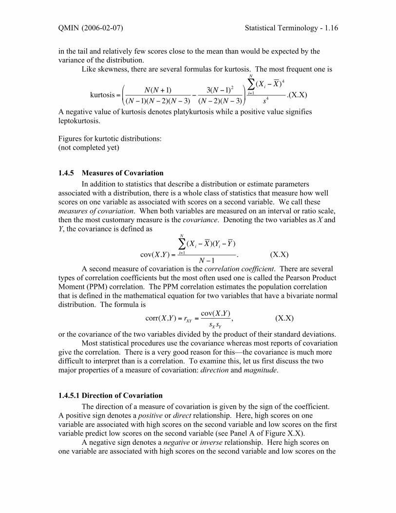
1.4.4 Measures of Peakness/FlatnessThe final attribute of a distribution is called kurtosis and is the extent to which

scores, relative to the variance of the distribution, are concentrated close to the mean (a“peaked” distribution) or are disproportionately present in the tails (a “flat” distribution).The three curves in Figure X.X illustrate kurtosis. The curve with the solid line is anormal curve. The curve with the short dashed lines illustrates a peaked distributionknown in statistical jargon as a leptokurtotic distribution after the Greek word leptos,meaning “thin.” A leptokurtotic distribution has relative more scores close to the meanand relatively fewer scores in the tails of the distribution that would be expected giventhe variance of the distribution.

The curve in Figure 1 with the longer dashed lines is a platykurtotic curve, namedfrom the Greek word platys, meaning broad or flat. Here, there are relatively more scores


in the tail and relatively few scores close to the mean than would be expected by thevariance of the distribution.

Like skewness, there are several formulas for kurtosis. The most frequent one is

€

kurtosis =N(N +1)

(N −1)(N − 2)(N − 3)−

3(N −1)2

(N − 2)(N − 3)

(Xi − X )4i=1

N

∑s4

.(X.X)

A negative value of kurtosis denotes platykurtosis while a positive value signifiesleptokurtosis.

Figures for kurtotic distributions:(not completed yet)

1.4.5 Measures of CovariationIn addition to statistics that describe a distribution or estimate parameters

associated with a distribution, there is a whole class of statistics that measure how wellscores on one variable as associated with scores on a second variable. We call thesemeasures of covariation. When both variables are measured on an interval or ratio scale,then the most customary measure is the covariance. Denoting the two variables as X andY, the covariance is defined as

€

cov(X,Y ) =

(Xi − X )(Yi −Y )i=1

N

∑N −1

. (X.X)

A second measure of covariation is the correlation coefficient. There are severaltypes of correlation coefficients but the most often used one is called the Pearson ProductMoment (PPM) correlation. The PPM correlation estimates the population correlationthat is defined in the mathematical equation for two variables that have a bivariate normaldistribution. The formula is

€

corr(X,Y ) = rXY =cov(X,Y )sX sY

, (X.X)

or the covariance of the two variables divided by the product of their standard deviations.Most statistical procedures use the covariance whereas most reports of covariation

give the correlation. There is a very good reason for this—the covariance is much moredifficult to interpret than is a correlation. To examine this, let us first discuss the twomajor properties of a measure of covariation: direction and magnitude.

1.4.5.1 Direction of CovariationThe direction of a measure of covariation is given by the sign of the coefficient.

A positive sign denotes a positive or direct relationship. Here, high scores on onevariable are associated with high scores on the second variable and low scores on the firstvariable predict low scores on the second variable (see Panel A of Figure X.X).

A negative sign denotes a negative or inverse relationship. Here high scores onone variable are associated with high scores on the second variable and low scores on the


first variable predict high scores on the second variable. Panel B of Figure X.X depicts anegative or inverse relationship.

1.4.5.2 Magnitude of CovariationThe magnitude of covariation measures the strength of the relationship between

the two variables. The problem with using the covariance as an index of magnitude isthat its value depends on the scale of the two variables. Consequently, given twocovariances, say .012 and 12,000, it is impossible to way which of them indicates astronger relationship.

The correlation coefficient, on the other hand, is independent of the scales of thetwo variables. Hence, it is the preferred statistic for reporting covariation. Thecorrelation has a natural mathematical lower bound of –1.0 and an upper bound of 1. Acorrelation of 0 implies no statistical relationship between the two variables. That is,neither of the variables can predict the other better than chance. A correlation of 1.0denotes a perfect, positive relationship. If we know an observation’s score on onevariable, then we can predict that observation’s score on the second variable withouterror. A correlation of –1.0 denote a perfect, but negative relationship. Here, we can alsopredict an observation’s score on the second variable given the score on the firstvariable—it is just that a high score on the first variable will predict a low score on thesecond.

The best index of magnitude is the square of the correlation coefficient. Note thatsquaring removes the sign so that correlations of .60 and -.60 both have the same estimateof magnitude (.36). The square of the correlation measures the proportion of variance inone variable statistically explained by the other variable. In less jargonish terms, it givesthe extent to which knowledge of individual differences in one variable predict individualdifferences in the second variable. Note that these statements have been deliberatelyphrased is such cautious terms as “statistically explained” and “predict.” This is becausea correlation coefficient has no causal implications. If X is correlated with Y, then: (1) Xmay cause (or be one of several causal factors of) Y; (2) Y may cause (or be one ofseveral causal factors of) X; (3) X and Y because are both caused by the same (or some ofthe same) factors; and (4) any combination of situations 1, 2, and 3 may occur.

1.5 Other Terms

1.5.1 OutliersAn outlier is defined as a data point that is well separated from the rest of the data

points. Velleman (19xx) divides outliers into two types, blunders and rouges. A blunderis a data point resulting from instrument, measurement, or clerical error. For example,IQ, a staple of the neuropsychological test battery, is typically scaled so that thepopulation mean is 100 and the population standard deviation is 15. A transposition errorin data entry may record an IQ of 19 in a database instead of the correct value of 91.Note that a blunder does not always result in an outlier—transposing an IQ score of 98,for instance, will not give a score disconnected from the IQ distribution. Blunders,however, are easily detected and corrected by following recommended practice and


having data entered twice. A comparison of the results from the first entry with those inthe second entry will almost always catch clerical data-entry errors.

A rouge, on the other hand, is a legitimate data value that just happens to beextreme. In clinical neuropsychology, for example, it is not unusual to encountersomeone with an extremely low IQ score because of a gross genetic or environmentalinsult to the central nervous system. What should be done with rouge data pointsdepends entirely on the purpose at hand. On the one hand, the observation(s) shouldnever be deleted from the data set because they can provide very important information.For example, in a meta-analysis5 of data on the genetics of human aggression, Miles &Carey (199x) found that the two rouge values were the only two studies that measuredaggression in the laboratory—all other studies used self-report questionnaires. On theother hand, the presence of a single rouge value in some statistical procedures can resultin very misleading inference. Here, there are three possible solutions: (1) temporarily setthe rouge value to missing value for the analysis; (2) transform the data; or (3) use anonparametric procedures that is not sensitive to outliers. We discuss these later in thecontext of statistical procedures.

Although we have spoken of rouges as applying to a single variable, it is possibleto have a multivariate rouge. This is a data point that might not be detected as a rougewhen each variable is examined individually but emerges as an outlier when the variablesare considered together. The classic example of a multivariate rouge would be ananorexic woman who is 5’10” tall and weighs 95 pounds. She is not remarkable in eitherheight taken alone or weight taken alone, but she would be an outlier in terms of the jointdistribution of height and weight.

1.5.2 Effect Size(not yet written)

1.5.3 Statistical Power (not yet written)

5 A meta-analysis is a systematic statistical analysis of a series of empirical studies.

1 statistical terminology and descriptive...

Documents