1

User-friendly SAS® Macro Application for performing all possible mixed modelselection - An update

George Fernandez, University of Nevada - Reno, Reno NV 89557

ABSTRACT

A user-friendly SAS macro application to perform all possible model selection of fixed effects including quadratic and cross products within a user-specified subset range in the presence ofrandom and repeated measures effects using SAS PROC MIXED is available. This macroapplication, ALLMIXED2 will complement the model selection option currently available in theSAS PROC REG for multiple linear regressions and the experimental SAS procedureGLMSELECT that focuses on the standard independently and identically distributed generallinear model for univariate responses. Options are also included in this macro to select the bestcovariance structure associated with the user-specified fully saturated repeated measuresmodel; to graphically explore and to detect statistical significance of user specified linear,quadratic, interaction terms for fixed effects; and to diagnose multicollinearity, via the VIFstatistic for each continuous predictors involved in each model selection step. Two modelselection criteria, AICC (corrected Akaike Information Criterion) and MDL (minimal descriptionlength) are used in all possible model selection and summaries of the best model selection arecompared graphically. The differences in the degree of penalty factors associated with themodel dimension between AICC and MDL are investigated. Complete mixed model analysis offinal model including data exploration, influential diagnostics, and checking for model violationsusing the experimental ODS GRAPHICS option available in Version 9.13 is also implemented.The ALLMIXED2 SAS macro application is an improved version of the SAS macro applicationALLMIXED2 previously reported (Fernandez, 2007). Instructions for downloading and runningthis user-friendly macro application are included.

INTRODUCTION

Model selection is usually carried out by the automated procedures built into the softwareincluding frequently used forward, backward, and stepwise model selection procedures. Thereis an extensive review and discussion on the theoretical aspects of model selection criteria andprocedures (Burnham and Anderson 2002; Hoeting et.al 2006). All possible model selection offixed effects in general linear model setup using delta AICC , delta SBC and model weights areimplemented in the REGDIAG macro (Fernandez, 2002). However, all possible mixed modelselection can be tedious, time consuming and complicated due to the presence of additionalrandom terms and optimal variance-covariance structure associated with repeated measures (Littell et.al 2006; Hoeting et.al 2006; Kramer 2004). Ngo and Rand (2002) developed a SASmacro for performing mixed model selection for user-specified models. Keselman et .al (1998)proposed a SAS based method to select the best covariance structure in mixed model repeatedmeasures analysis. However, to apply these SAS macros in model selection, SASprogramming experience is a requirement. Kramer (2004) developed an automated modelselection application using SAS Mixed and PERL codes for both fixed and random effects. Programming knowledge in PERL is required to use this application. This paper presents apractical and complete solution for automated and efficient mixed model selection and model

2

exploration using a user-friendly SAS macro application named ALLMIXED2. The ALLMIXED2SAS macro application presented here is an improved version of the SAS macro applicationALLMIXED2 previously reported elsewhere (Fernandez, 2007). All new improvements of thepreviously reported ALLMIXED2 macro applications are emphasized here.

MODEL SELECTION CRITERIA USED IN ALLMIXED2 MACRO

The general form of information criterion (IC )= -2 log L + Penalty factor (pf)

-2 log L is derived from PROC MIXED method = ML

∆ -2 log L = (-2 log L I )- (-2 log L min )

-2 log L min = The smallest -2 log L derived from PROC MIXED method ML of all models compared.

AIC = -2 log L + 2(p+k+1) ( Hoeting et. al 2006)

AICC= -2 log L + [2(p+k+1) (n/(n-p-k-2))] ( Hoeting et. al 2006)

Where p = number of fixed effect terms k = number of random effect terms n = total sample size for random effect model and number of subjects in case of repeatedmeasures * In large sample AIC and AICC are nearly equivalent

∆AICC = AICCi- AICC min Best candidate models = (∆AICC <=2)

AICCsas = AICC reported by SAS PROC Mixed using ML

AICCREML = AICC reported by SAS PROC Mixed using REML

MDL =1/2 {-2 log L + [log(n) (p+k+1)]} ( Hoeting et. al 2006)

∆ MDL = MDLi- MDL min Best candidate models = (∆ MDL <=1) In the ALLMIXED2 macro, the best candidate models selection criterion based on MDL is changed from1/2(log(n)) (Fernandez 2006) to <=1. This new criterion is comparable to the criterion used for AICC (<=2)

BIC = -2 log L + [log(n) (p+k+1)] (SAS Institute 2006)

Penalty factor % = (pf i / -2 log L ref) *100

-2 log L ref = -2 log L derived from PROC MIXED method ML that contain optional random and repeatedmeasure covariance parameter and user specified “Must-Have” fixed effects.

AICC weights =Exp(-0.5*Delta AICC i) / Sum of (Exp(-0.5*Delta AICC i) ) all best candidate model (Buckland et al. 1997).MDL weights =Exp(-0.5*Delta MDL i) / Sum of (Exp(-0.5*Delta MDL i) ) all best candidate model AICC weight ratio = AICC weight / Max (AICC weight)MDL weight ratio = MDL weight / Max (MDL weight)

3

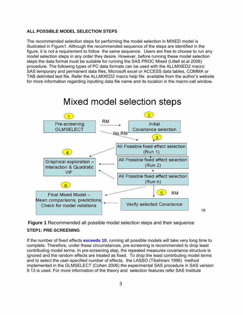
ALL POSSIBLE MODEL SELECTION STEPS

The recommended selection steps for performing the model selection in MIXED model isillustrated in Figure1. Although the recommended sequence of the steps are identified in thefigure, it is not a requirement to follow the same sequence. Users are free to choose to run anymodel selection steps in any order they desire. However, before running these model selectionsteps the data format must be suitable for running the SAS PROC Mixed (Littell et.al 2006)procedure. The following types of PC data formats can be used with the ALLMIXED2 macro:SAS temporary and permanent data files, Microsoft excel or ACCESS data tables, COMMA orTAB delimited text file. Refer the ALLMIXED2 macro help file available from the author’s websitefor more information regarding inputting data file name and its location in the macro-call window.

STEP1: PRE-SCREENING

If the number of fixed effects exceeds 10, running all possible models will take very long time tocomplete. Therefore, under these circumstances, pre-screening is recommended to drop leastcontributing model terms. In pre-screening step, the repeated measures covariance structure isignored and the random effects are treated as fixed. To drop the least contributing model termsand to select the user-specified number of effects, the LASSO (Tibshirani 1996) methodimplemented in the GLMSELECT (Cohen 2006) the experimental SAS procedure in SAS version9.13 is used. For more information of the theory and selection features refer SAS Institute

Figure 1 Recommended all possible model selection steps and their sequence

4

(2006). The LASSO model selection options - CHOOSE=NONE and SELECT=SBC are used inthis macro. The ‘FIT CRITERIA" and the ‘COEFFICIENT EVALUATION' plots generated by theSAS ODS GRAPHICS features were utilized in the pre-screening evaluation to identify thepotential subset ranges and to drop potential insignificant covariate and to select less than orequal to 10 potentially significant covariates.

The LASSO selection method add or drop an effect and compute several information criteria (IC)statistics in each step. The FIT CRITERIA plots display the trend of six IC statistics in each stepand the best subset is identified by a STAR symbol (Figure 2). Because, the SELECT=SBCoption was used, the FIT CRITERIA plot highlight the best subset based on the SBC criterion. The ‘COEFFICIENT EVALUATION’ plots displayed in Figure 3, shows the magnitude of thestandardized regression coefficients of the selected model effects in each step along with the SBC criterion. This plot could help us to discard the not contributing effects and to select less than or equal 10covarites which can be used in the all possible mixed model selection in the next step.

STEP2: REPEATED MEASURES - INITIAL COVARIANCE TYPE SELECTION.In a repeated measures modeling , the best covariance structure describing the correlationamong the repeated measures should be identified first. The best covariance structure can beidentified from different user-specified covariance structures by comparing the AICC statisticcomputed in PROC MIXED using REML method and select the covariance type which gives thesmallest AICC value. Refer the ALLMIXED2 macro help file available from the authors websitefor more information regarding inputting appropriate parameters.

Step3: All possible model selection steps

All combination of models associated with the user-specified fixed effects subset range (start:2and stop:6) are generated by the ALLMIXED2 macro and their information criteria statistics, AICCand MDL are compared in this step. Users can optionally specify certain fixed effects as “MUSTHAVE” and other fixed effects as “SELECTABLE” in the all possible model selection. Allcombination of mixed model using the fixed effects listed in “SELECTABLE” category aregenerated in this step and the following statistics are estimated.Variance inflation statistics (VIF) for each continuous predictor variables in the model.PRESS statistics generated in GLM proc- To monitor the impact of influential observations thedifferences between PRESS and SSE are evaluated in each model selection step.Information criteria estimates based on REML: AICCremlInformation criteria estimates based on ML: AIC, AICC, AICCsas, MDL, and BIC.

In the ALLMIXED2 macro, the following changes are made in the computation of the ICstatistics. When computing the IC statistics for a repeated measures data during the pre-screening and the all possible subset model selection step, the sample size (n=250) issubstituted by the number of subjects (50). Thus, the results reported in this paperregarding the performance of AICC and MDL in model selection is contradicting with thepreviously reported results (Fernandez, 2006) for the same data where a larger samplenumber N=250 was used.

5

Figure 3 Standardized regression coefficient estimates and SBC computed at each model selectionsequence during the LASSO method of model selection available in SAS procedure GLMSELECT. The modelparameters included are two group effects (trt and time) and 20 covariates (x1-x20)

Figure 2 Information criteria estimates computed in the LASSO method of model selection available in SASprocedure GLMSELECT. The model parameters included are two group effects (trt and time) and 20covariates (x1-x20)

6

The relationships between AIC, AICC, AICCsas, AICCreml, MDL, and BIC can be investigated bythe rank correlations using the SAS PROC CORR and scatter plot matrix (Figure 5). Perfect rankcorrelations (1) are commonly observed between (AICC and AICCsas ) and (MDL and BIC) indicating that these two sets of IC behave identically in the model selection. Furthermore AICand AICC doesn’t behave similarly and the degree of penalty is not the same when the numberof fixed effects is relatively larger (p=19) compared with total number of observations (n=numberof subjects= 50).

All IC statistics reported here are made out of two components: Log likelihood estimate (-2 log L )and penalty factor (pf). For a given model, -2log L value is constant and is influenced by degree ofmodel fit, variable included and not included in the model, presence of influential outliers, andmodel specification errors. The penalty factor is made out of number of fixed (p) and randomeffects (k) and the sample size (n). When all possible model selection involving only the fixedeffects are carried out, the sample size and the number of random effects become constant.Therefore, only the number of fixed factor becomes the determining component of the penaltyfactor. The relationship between penalty factor and the number of fixed effects between AIC_C,

Figure 4 Repeated Measure analysis covariance type selection based on smallestAICC.

7

AICCreml, and MDL are shown in Figure 6. The penalty factor for the AICCreml becomes constantbecause this penalty factor does not include any fixed effects and only the number of randomeffects (which is a constant) is included.

The components of AICC and MDL ( -2 log l and the penalty factor) are graphically compared inFigure 7. For a given model, -2log L value is constant when estimating AICC and MDL and itdecreases linearly with an increase in the number of fixed terms. But, within a subset (two, three,four variable subset), the -2 log L value varies a lot whereas all the models within a subset havethe same penalty factor for both AICC and MDL (Figure 7). Also AICC statistic favorsparsimonious model (2 and 3 subsets) whereas MDL statistic favors models with large number ofmodel terms (3,4,5 subsets) especially in a small data set (50 subjects in repeated measuresdata) (Figure 7).This contradicts with the earlier report where MDL favored more parsimoniousmodels when n was considered large (50 subjects x 5 repeated measures =total sample size 250)Fernandez (2006)

Graphical display of best models within each subset based on smallest ∆AICC and ∆MDL withineach subset are shown in Figure 8. Graphical display of overall best candidate models based on ∆AICC <= 2 and ∆MDL <=1 are shown in Figure 9. Refer the ALLMIXED2 macro help file available from the authors website for more information regarding downloading this user-friendlymacro file and associated macro help file.

Figure 5 Scatter plot matrix showing rank correlation among 4 AIC and 2 BC based Information criteriastatistics in all possible mixed model selection

8

inputting appropriate parameters in the macro-call window.

Figure 7 Comparison of the association between AICC and MDL components and thenumber of fixed effect terms

Figure 6 Comparison of penalty factor among AICC, AICC reml and MDL versus numberof fixed effect terms.

9

STEP4: GRAPHICAL EXPLORATION FOR MULTICOLLINARITY AND MODEL

Figure 8 Graphical display of best model within each subset identified by the AICCand MDL

Figure 9 Graphical display of best candidate models identified by AICC (<=2) and theMDL (<=1).

10

SPECIFICATION ERROR

Severe multicollinarity (Variance inflation factor > 10) among predictor variables in mixed modelanalysis can result in unstable parameter estimates with inflated standard errors. When a fixedeffect predictor involved in a collinear relationship is dropped from the model, the sign and size ofthe remaining predictor variable estimates can change dramatically. Therefore, presence of highdegree of multicollinarity can impact fixed effect selection. Therefore, assessing the degree ofmulticollinarity for each of the continuous fixed effects in all possible model selection can help toselect the best model from the set of best candidate models. Variable(s) not contributingmulticollinarity could be preferred over the variables significantly contributing to multicolliniarity.Figure 10 shows the box-plot display of VIF distribution for all the continuous predictors includedin model selection. Also, to diagnose multicollinearity in each model selection step (when VIFvalue > 10) the VIF statistic for each continuous predictors involved in multicollinarity is sent toan excel output table for further exploration.

11

Model selection success can also be influenced by model specification error when significanthigher order model terms (quadratic and cross-product) omitted from the mixed model. The needfor an quadratic term or an interaction between any two predictor variables could be evaluated inthe 'quadratic’ or ‘interaction detection plot respectively. To detect the need for a significantquadratic term, first fit the full model including the quadratic term for the given predictor variable(Xi) and examine the Type III P-value for statistical significance and output the predicted values(YHATfull) for the full model. Then drop both the linear and the quadratic terms for this givenpredictor from the model and estimate the predicted values for this reduced model (YHATred).Then a graphical display between the ∆yhat (YHATfull -YHATred) and Xi can reveal the nature andthe strength of quadratic effects (Figure 11).

Similarly, to detect the need for a significant interaction term between two predictors, first fit thefull model including the cross-product term for the two predictor variable (X1 and X2) and examinethe Type III P-value for statistical significance of the interaction term and output the predictedvalues (YHATfull) for the full model. Then drop the cross product from the model and estimatethe predicted values for this reduced model (YHATred). Then a 3-D graphical display between the∆yhat (YHATfull -YHATred) and X1 and X2 can reveal the nature and the strength of interactioneffects (Figure 12). Refer the ALLMIXED2 macro help file available from the authors website)for more information regarding inputting appropriate parameters in the macro-call window.Step5: Final covariance type selection.(Optional step- for repeated measures model)

After several runs of all possible model selection steps, many data exploration, influentialobservation and multicollinarity checks, we can select the final fixed effect model. But, beforefinalizing the final mixed effect model it is important to verify whether the covariance type used inthe model selection step is still the best type for the selected model. Again user-specifiedcovariance types, can be compared and the final covariance type selection can be made basedon ∆AICCj (AICCj - AICC min) using PROC MIXED REML method. Refer the ALLMIXED2 macrohelp file available from the authors website) for more information regarding inputting appropriateparameters in the macro-call window.

Step6: Complete mixed model analysis

After selecting the final repeated measures mixed model dimensions, complete mixed modelanalysis can be performed including the data exploration by box plots (Figure 13), mixed modelanalysis, LSMEAN comparisons with alphabet mean separation ( Figure 14-15) suggested bySaxton (2002), model predictions, checking for normality of studentized conditional residuals(Figure 16), and performing influential diagnostics (Figure 17) in one step. Refer theALLMIXED2 macro help file available from the authors website for more information regardinginputting appropriate parameters in the macro-call window.

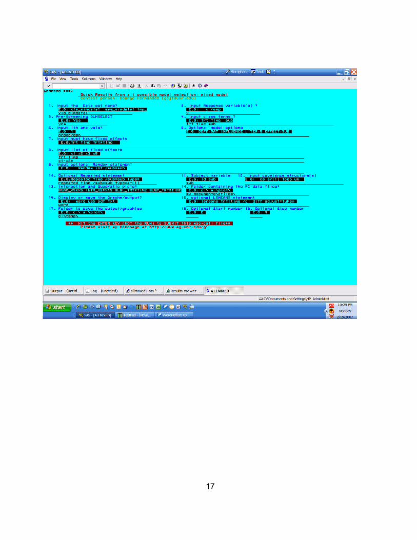
AVAILABILITY OF THE ALLMIXED2 MACRO:Users can download the ALLMIXED2 .SAS macro-call file from the authors website athttp://www.ag.unr.edu/gf and by clicking the “Running puppy dog” clip art. Save the ALLMIXED2.SAS macro-call file in your PC first and open it in SAS display manager and submit to view theblue macro-call window (Figure 18) (You need to have access to INTERNET to download andexecute the macro while running this ALLMIXED2 macro in your system). Input all the requiredmacro input parameters and submit the macro to perform the all possible mixed model selection.Please refer the required SAS modules listed below for running this macro successfully.

12

Figure 11 Graphical exploration and the statistical significance of the user-specifiedquadratic effect.

Figure 12 Graphical exploration and the statistical significance of the user-specifiedcross product

13

Figure 13 Mixed model violation detection using studentized conditional residuals

14

Figure 14 Exploration of repeated measures-Time effect by box plot

Figure 15 Main effect LSMEAN Comparison - using alphabet notation

15

Figure 16 LSMEAN Comparison - Interaction means with alphabet notations

16

Figure 17 Repeated measurers mixed model influential diagnostics - at the subjectlevel

17

18

Required SAS Modules for Running the All mixed SAS Macro in Version 9.13:

! SAS /STAT : PROCS MIXED, CORR, REG and GLMSELECT! SAS/GRAPH: PROC GCHART, PROC GPLOT, PROC G3D! SAS/BASE SAS ODS (RTF, HTML, PDF)! SAS/ACCESS: PC FILES – PROC IMPORT and EXPORT

SUMMARY

The main features of the user-friendly SAS macro application, ALLMIXED2 are summarizedbelow:

• The users can input, temporary and permanent SAS data files, Microsoft Excel andAccess and comma and TAB delimited text files as input data set.

• Users can input multiple response variables and perform all the model selection stepssimultaneously.

• Users can optionally pre-screen the fixed effects and drop obvious non-significant fixedeffects if the number of fixed effects exceed 10 using the SAS 9.13 experimental GLMSELECT procedure implemented within the macro. The new model selectionmethod, LASSO is used in this macro to pre-screen the many fixed effects.

• In case of repeated measures mixed model analysis, the best covariance structureselection from the user specified covariance structures are implemented by comparingthe AICC value estimated in the Proc Mixed using REML method and then bestcovariance structures is graphically identified by searching for the covariance structurewith the smallest AICC value.

• Options for performing all possible fixed effect model selection with and without repeatedand random effects and selecting the best candidate models using AICC and MDLestimates using PROC MIXED method ML. In this step, users can differentiate the “must-keep” effects and “selectable” effects. The all possible model selection will be performedusing the fixed effects identified in the “Selectable” list of terms.

• Best candidates models can be selected by the delta AICC and delta MDL based modelweight statistics.

• Options are also available for graphical exploration and statistical significance of userspecified linear, quadratic, interaction terms for fixed effects. Also, to diagnosemulticollinearity (when VIF value > 10) the VIF statistic for each continuous predictorsinvolved in each model selection step are sent to an output table. Also, a boxplot displayof VIF estimates by all the continuous fixed effects are generated for the overallassessment of multicollinarity in the model selection process.

• Options are also available for performing complete mixed model analysis of final modelincluding data exploration, influential diagnostics, and checking for model violations usingthe experimental ODS GRAPHICS option available in Version 9.13.

• Users can save all SAS output and graphics in Word, HTML, or PDF formats. Inaddition, full details all model selection diagnostic statistics are automatically sent to MSexcel data tables. SAS log messages are automatically saved to external text log filesand only the ERROR and WARNING messages are extracted and displayed as HTMLoutput for easy error checks.

• Download instructions are given above to download this macro-call file and to perform allpossible model selection.

19

REFERENCES1. Buckland, S. T., K. P. Burnham, and N. H. Augustine. 1997. Model selection: an integral partof inference. Biometrics 53:603-618.2. Burnham, K. P, and Anderson D. R. (2002) Model selection and inference: a practical information theoretic approach. (Second edition) Springer-Verlag, New York, New York, USA.3. Cohen R. A (2006) Introducing the GLMSELECT PROCEDURE for Model Selection SUGI31proceedings http://www2.sas.com/proceedings/sugi31/207-31.pdf4. Efron, B., Hastie, T., Johnstone, I., and Tibshirani, R. (2004), “Least Angle Regression (withdiscussion), Annals of Statistics, 32, 407–499.5. Fernandez, G (2002) Data Mining using SAS applications Book 384 p CRC-Chapman Hall FLUSA 6. Fernandez, G 2006. Model Selection Methods in PROC MIXED Proceeding of Western SASusers conference San Francisco CA.http://www.lexjansen.com/wuss/2006/Analytics/ANL-Fernandez.pdf7. Fernandez, G 2007. Model Selection in PROC MIXED - A User-friendly SAS® MacroApplication SAS Global Forum http://www2.sas.com/proceedings/forum2007/191-2007.pdf Paper 191-20078. Hoeting, J.A, Davis R.A Merton A.A and Thompson S. E (2006) Model selection for Geostatistical Models Ecological Applications, 16(1), pp. 87–989. Keselman, H. J., Algina, J., Kowalchuk, R. K., and Wolfinger, R. D. (1998) A comparison oftwo approaches for selecting covariance structures in the analysis of repeated measurement,27, Communications in Statistics, Simulation & Computation 591-604.10. Littell, R.C, Milliken, G A., Stroup, WW, and Wolfinger, R D. (2006). SAS System for MixedModels (second edition) , Cary, NC: SAS Institute Inc.11. Kramer M (2004) Automatic model selection in the mixed model framework KSU appliedstatistics conference proceedings 12. Ngo, L and Rand, R. (2002). Model Selection in Linear Mixed Effects Models Using SAS®Proc Mixed. SUGI 22 http://www2.sas.com/proceedings/sugi22/STATS/PAPER284.PDF13. SAS Institute (2006) The GLMSELECT procedure (Experimental) Cary, NC http://support.sas.com/rnd/app/papers/glmselect.pdf14. Saxton, A.M A Macro for Converting Mean Separation Output to Letter Groupings in PROCMIXED SUGI23 http://www2.sas.com/proceedings/sugi23/Stats/p230.pdf15. Tibshirani, R. (1996) Regression Shrinkage and Selection via the Lasso Journal of theRoyal Statistical Society Series B, 58, 267–288

CONTACT INFORMATION

Your comments and questions are valued and encouraged. Contact the author:

Name: George C. Fernandez, PhD Enterprise: Director / CRDA University of Nevada - RenoAddress: CRDA/088 Reno, NV 89557Work phone: (775)-784-4206 Email: gcjf@unr.edu Web: Http://www.ag.unr.edu/gfSAS and all other SAS Institute Inc. product or service names are registered trademarks or trademarks ofSAS Institute Inc. in the USA and other countries. ® indicates USA registration. Other brand and product names are trademarks of their respective companies.