1

WHAT COMES TO MIND1

Nicola Gennaioli and Andrei Shleifer

Sixth Draft, November 18, 2009

Abstract

We present a model of intuitive inference, called “local thinking,” in which an

agent combines data received from the external world with information retrieved from

memory to evaluate a hypothesis. In this model, selected and limited recall of

information follows a version of the respresentativeness heuristic. The model can

account for some of the evidence on judgment biases, including conjunction and

disjunction fallacies, but also for several anomalies related to demand for insurance.

Key words: local thinking, representativeness, stereotypes, insurance

1 We are deeply grateful to Josh Schwartzstein for considerable input, and to Pedro Bordalo, Shane Frederick, Xavier Gabaix, Matthew Gentzkow, Daniel Hojman, Elizabeth Kensinger, Daniel Kahneman, Lawrence Katz, Scott Kominers, David Laibson, Sendhil Mullainathan, Giacomo Ponzetto, Drazen Prelec, Mathew Rabin, Antonio Rangel, Jesse Shapiro, Jeremy Stein, Richard Thaler, and three anonymous referees for extremely helpful comments. Gennaioli thanks the Spanish Ministerio de Ciencia y Tecnologia (ECO 2008-01666 and Ramon y Cajal grants), the Barcelona GSE Research Network and the Generalitat de Catalunya for financial support. Shleifer thanks the Kauffman Foundation for research support.

2

1. Introduction

Since the early 1970s, Daniel Kahneman and Amos Tversky (hereafter KT 1972,

1974, 1983) published a series of remarkable experiments documenting significant

deviations from the Bayesian theory of judgment under uncertainty. While KT’s

heuristics and biases program has survived substantial experimental scrutiny, models of

heuristics have proved elusive.2 In this paper, we present a memory based model of

probabilistic inference that accounts for quite a bit of the experimental evidence.

Heuristics describe how people evaluate hypotheses quickly, based on what first

comes to mind. People may be entirely capable of more careful deliberation and analysis,

and perhaps of better decisions, but not when they do not think things through. We

model such quick and intuitive inference, which we refer to as “local thinking,” based on

the idea that only some decision-relevant data come to mind initially.

We describe a problem in which a local thinker evaluates a hypothesis in light of

some data, but with some residual uncertainty remaining. The combination of the

hypothesis and the data primes some thoughts about the missing data. We refer to

realizations of the missing data as scenarios. We assume that working memory is limited,

so that some scenarios, but not others, come to the local thinker’s mind. He makes his

judgment in light of what comes to mind, but not of what does not.

Our approach is consistent with KT’s insistence that judgment under uncertainty

is similar to perception. Just as an individual fills in details from memory when

interpreting sensory data (for example, when looking at the duck-rabbit or when judging

distance from the height of an object), the decision maker recalls missing scenarios when

2 Partial exceptions include Griffin and Tversky (1992), Tversky and Koehler (1994), Barberis et al. (1998), Rabin and Schrag (1999), Mullainathan (2000), and Rabin (2002), to which we return in Section 3.3.

3

he evaluates a hypothesis. Kahneman and Frederick (2005) describe how psychologists

think about this process: “The question of why thoughts become accessible – why

particular ideas come to mind at particular times – has a long history in psychology and

encompasses notions of stimulus salience, associative activation, selective attention,

specific training, and priming (p. 271).”

Our key assumption describes how scenarios become accessible from memory.

We model such accessibility by specifying that scenarios come to mind in order of their

representativeness, defined as their ability to predict the hypothesis being evaluated

relative to other hypotheses. This assumption formalizes aspects of KT’s

representativeness heuristic, modelling it as selection of stereotypes through limited and

selective recall. The combination of both limited and selected recall drives the main

results of the paper, and helps account for biases found in psychological experiments.

In the next section, we present an example illustrating the two main ideas of our

approach. First, the data and the hypothesis being evaluated together prime the recall of

scenarios used to represent this hypothesis. Second, the representative scenarios that are

recalled need not be the most likely ones, and it is precisely in those instances when a

hypothesis is represented with an unlikely scenario that judgement is severely biased.

In Section 3, we present the formal model, and compare it to some earlier

theoretical research on heuristics and biases.

In section 4, we present the main theoretical results of the paper, and establish

four propositions. The first two deal with the magnitude of judgment errors. Proposition

1 shows how judgment errors depend on the likelihood of the recalled (representative)

scenarios. Proposition 2 then shows how a local thinker reacts to data, and in particular

4

overreacts to data that change his representation of the hypothesis he evaluates. The next

two propositions deal with perhaps the most fascinating judgment biases, namely failures

of extensionality. Proposition 3 describes the circumstances in which a local thinker

exhibits the conjunction fallacy, the belief that a specific instance of an event is more

likely than the event itself. Proposition 4 then shows how a local thinker exhibits the

disjunction fallacy, the belief that the combined probability of several independent events

is lower than the sum of the probabilities of the constituent events.

In section 5, we show how the propositions shed light on a range of experimental

findings on heuristics and biases. In particular, we discuss the experiments on the neglect

of base rates, insensitivity to predictability, as well as the conjunction and disjunction

fallacies. Among other things, the model accounts for the famous Linda (KT 1983) and

car mechanic (Fischhoff, Slovic, and Lichtenstein 1978) experiments.

In section 6, we apply the model, and in particular its treatment of the disjunction

fallacy, to individual demand for insurance. Cutler and Zeckhauser (2004) and

Kunreuther and Pauly (2005) summarize several anomalies in that demand, including

over-insurance of specific narrow risks, under-insurance of broad risks, and preference

for low deductibles in insurance policies. Our model sheds light on these anomalies.

Section 7 concludes by discussing some broader conceptual issues.

2. An Example: Intuitive Reasoning in an Electoral Campaign

We illustrate our model in the context of a voter’s reaction to a blunder committed

by a political candidate. Popkin (1991) argues that intuitive reasoning plays a key role in

this context and helps explain the significance that ethnic voters in America attach to the

5

candidates’ knowledge of their customs. He further suggests that, although in many

instances voters’ intuitive assessments work pretty well, they occasionally allow even

minor blunders such as the one described below to influence their votes.

“In 1972, during New York primaries, Senator George McGovern of South

Dakota was courting the Jewish vote, trying to demonstrate his sympathy for Israel. As

Richard Reeves wrote for New York magazine in August, ‘During one of McGovern’s

first trips into the city he was walked through Queens by city councilman Matthew Troy

and one of their first stops was a hot dog stand. “Kosher?” said the guy behind the

counter, and the prairie politician looked even blanker than he usually does in big cities.

“Kosher!” Troy coached him in a husky whisper. “Kosher and a glass of milk,” said

McGovern.” (Popkin, 1991, p. 2). Evidently, McGovern was not aware that milk and

meat cannot be combined in a kosher meal.

We use this anecdote to introduce our basic formalism and to show how “local

thinking” can illuminate the properties of voters’ intuitive assessments. We start with the

case in which intuitive assessments work well, and then return to hotdogs.

Suppose that a voter only wants to assess the probability that a candidate is

qualified. Before he hears the candidate say anything, he assesses this probability to be

1/2. Suppose that the candidate declares at a Jewish campaign event that Israel was the

aggressor in the 1967 war, an obvious inaccuracy. How does the voter’s assessment

change? For a Bayesian voter, the crucial question is the extent to which this statement –

which surely signals the candidate’s lack of familiarity with Jewish concerns – is also

informative about the candidate’s overall qualification. Suppose that the distribution of

candidate types conditional on calling Israel the aggressor is described by Table I.A:

6

Calls Israel aggressor in 1967 war

Familiarity with Jewish Concerns familiar unfamiliar

qualification of candidate

qualified

0.15

0.025

unqualified

0.025

0.8

Table I.A

Not only is “calling Israel the aggressor in the 1967 war” very informative about a

candidate’s unfamiliarity with Jewish concerns (82.5% of the candidates who say this are

unfamiliar), but unfamiliarity is in turn very informative about qualification, at least to a

Jewish voter (relative to a prior of 1/2 before calling Israel aggressor). The latter

property is reflected in the qualification estimate of a Bayesian voter, which is equal to:

Pr(qualified) = Pr(qualified, familiar) + Pr(qualified, unfamiliar) = 0.175, (1)

where we suppress conditioning on “calling Israel aggressor”. The Bayesian reduces his

assessment of qualification from 50% to 17.5% because the blunder is so informative.

Suppose now that Table I.A, rather than being immediately available to the voter,

is stored in his associative long term memory and that – due to working memory limits –

not all candidate types come to mind to aid the voter’s evaluation of the candidate’s

qualification.3 We call such a decision maker a “local thinker” because, unlike the

Bayesian, he does not use all the data in Table I.A, but only the information he obtains by

sampling from memory specific examples of qualified and unqualified candidates.

Crucially, we assume in KT’s spirit that the candidates who first come to the

voter’s mind are representative, or stereotypical, qualified and unqualified candidates.

Specifically, the voter’s mind automatically fits the most representative familiarity level –

or “scenario” – for each level of qualification of the candidate. We formally define the

3 Throughout the paper, we take the long term associative memory database (in this example, Table I.A) as given. Section 3 discusses how, depending on the problem faced by the agent, such a database might endogenously change and what could be some of the consequences for judgments.

7

representative scenario as the familiarity level that best predicts, i.e. is relatively more

associated with, the respective qualification level. These representative scenarios for a

qualified and an unqualified candidate are then given by:

{ })Pr(maxarg)(

,squalifiedqualifieds

unfamiliarfamiliars∈= , (2)

{ })Pr(maxarg)(

,sdunqualifiedunqualifies

unfamiliarfamiliars∈= . (3)

In Table I.A, this means that a stereotypical qualified candidate is familiar with Jewish

concerns, whereas a stereotypical unqualified one is unfamiliar with such concerns.4 This

process reduces the voter’s actively processed information to the circled diagonal:

Calls Israel aggressor in 1967 war

Familiarity with Jewish Concerns familiar unfamiliar

qualification of candidate

qualified

0.15

0.025

unqualified

0.025

0.8

Table I.B

Since a local thinker considers only the stereotypical qualified and unqualified

candidates, his assessment (indicated by superscript L) is equal to:

158.0),Pr(),Pr(

),Pr()(Pr ≈+

=unfamiliardunqualifiefamiliarqualified

familiarqualifiedqualifiedL (4)

Comparing (4) with (1), we see that a local thinker does almost as well as a Bayesian.

The reason is that in Table I.A stereotypes capture a big chunk of the respective

hypotheses’ probabilities. Although the local thinker does not recall that some unfamiliar

candidates are nonetheless qualified, this is not a big problem for assessment because in

reality, and not only in stereotypes, familiarity and qualification largely go together.

4 Indeed, Pr(qualified|familiar)= (.15/(.15+.025)) =..86 > .14= (.025/(.15+.025)) =Pr(qualified|unfamiliar). The reverse is true for an unqualified candidate.

8

The same idea suggests, however, that sometimes local thinkers make very biased

assessments. Return to the candidate unaware that drinking milk with hotdogs is not

kosher. Suppose that, after this blunder, the distribution of candidate types is:

Drinks milk with a hotdog Familiarity with Jewish Concerns familiar unfamiliar

qualification of candidate

qualified

0.024

0.43

unqualified

0.026

0.52

Table I.C

As in the previous case, in Table I.C the candidate’s drinking milk with hotdogs is

very informative about his unfamiliarity with Jewish concerns, but now such

unfamiliarity is extremely uninformative about the candidate’s qualification. Indeed, 95%

of the candidates do not know the rules of kashrut, including the vast majority of both the

qualified and the unqualified ones. In this example a Bayesian assesses Pr(qualified) =

0.454; he realizes that drinking milk with a hotdog is nearly irrelevant for qualification.

The local thinker, in contrast, still views the stereotypical qualified candidate as

one familiar with his concerns and the stereotypical unqualified candidate as unfamiliar.

Formally, the scenario “familiar” yields a higher probability of the candidate being

qualified [.024/(.024+.026) = .48] than the scenario “unfamiliar” [.43/(.43+.52) = .45].

Likewise, the scenario unfamiliar yields a higher probability of the candidate being

unqualified (.55) than the scenario familiar (.52). The local thinker then estimates:

044.0),Pr(),Pr(

),Pr()(Pr ≈+

=unfamiliardunqualifiefamiliarqualified

familiarqualifiedqualifiedL (5)

9

which differs from the Bayesian’s assessment by a factor of nearly 10! In contrast to the

previous case, the local thinker grossly overreacts to the blunder and misestimates

probabilities. Now local thinking generates a massive loss of information and bias.

Why this difference in the examples? After all, in both examples the stereotypical

qualified candidate is familiar with the voter’s concerns, while the stereotypical

unqualified candidate is unfamiliar since, in both cases, familiarity and qualification are

positively associated in reality. The key difference lies in how much of the probability of

each hypothesis is accounted for by the stereotype.

In the initial, more standard, example, almost all qualified candidates are familiar

and unqualified ones are unfamiliar, so stereotypical qualified and unqualified candidates

are both extremely common. When stereotypes are not only representative but also

likely, the local thinker’s bias is kept down. In the second example, in contrast, the bulk

of both qualified and unqualified candidates are unfamiliar with the voter’s concerns,

which implies that the stereotypical qualified candidate (familiar with concerns) is very

uncommon while the stereotypical unqualified candidate is very common. By focusing

only on the stereotypical candidates, the local thinker drastically underestimates

qualification because he forgets that many qualified candidates are also unfamiliar with

the rules of kashrut! When the stereotype for one hypothesis is much less likely than that

for the other hypothesis, the local thinker’s bias is large.

Put differently, in our example, after seeing a blunder the local thinker always

downgrades qualification by a large amount because the stereotypical qualified candidate

is very unlikely to commit any blunder. This process leads to good judgments in

situations where the blunder is informative not only of the dimension defining the

10

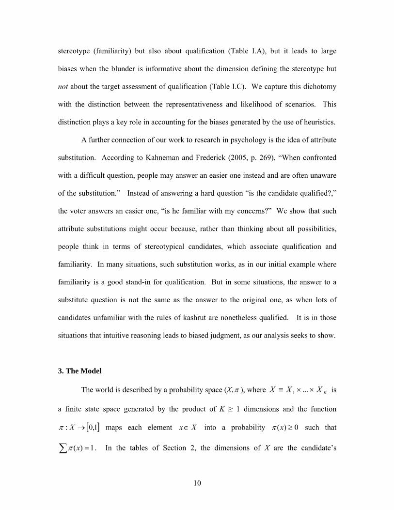
stereotype (familiarity) but also about qualification (Table I.A), but it leads to large

biases when the blunder is informative about the dimension defining the stereotype but

not about the target assessment of qualification (Table I.C). We capture this dichotomy

with the distinction between the representativeness and likelihood of scenarios. This

distinction plays a key role in accounting for the biases generated by the use of heuristics.

A further connection of our work to research in psychology is the idea of attribute

substitution. According to Kahneman and Frederick (2005, p. 269), “When confronted

with a difficult question, people may answer an easier one instead and are often unaware

of the substitution.” Instead of answering a hard question “is the candidate qualified?,”

the voter answers an easier one, “is he familiar with my concerns?” We show that such

attribute substitutions might occur because, rather than thinking about all possibilities,

people think in terms of stereotypical candidates, which associate qualification and

familiarity. In many situations, such substitution works, as in our initial example where

familiarity is a good stand-in for qualification. But in some situations, the answer to a

substitute question is not the same as the answer to the original one, as when lots of

candidates unfamiliar with the rules of kashrut are nonetheless qualified. It is in those

situations that intuitive reasoning leads to biased judgment, as our analysis seeks to show.

3. The Model

The world is described by a probability space (X,π ), where KXXX ××≡ ...1 is

a finite state space generated by the product of K ≥ 1 dimensions and the function

[ ]1,0: →Xπ maps each element Xx∈ into a probability 0)( ≥xπ such that

1)( =∑ xπ . In the tables of Section 2, the dimensions of X are the candidate’s

11

qualification and his familiarity with voter concerns, i.e. K = 2 (conditional on the

candidate’s blunder, which is a dimension kept implicit), the elements Xx∈ are

candidate types and the entries in the tables represent the probability measure π .

An agent evaluates the probability of 1>N hypotheses Nhh ,...,1 in light of data

d . Hypotheses and data are events of X. That is, rh (r = 1,..., N) and d are subsets of X.

If the agent receives no data, Xd = : nothing is ruled out. Hypotheses are exhaustive but

may be non-exclusive. Exhaustivity is not crucial, but avoids trivial cases where a

hypothesis is over-estimated simply because the agent cannot conceive of any alternative

to it. In (X,π), the probability of hr given d is determined by Bayes’ rule as:

∑∑

∈

∩∈=∩

=

dx

dhxrr x

x

ddh

dh r

)(

)(

)Pr()Pr(

)Pr(π

π. (6)

In our example, (1) follows from (6) since in Table I.A the probabilities are normalized

by Pr(calls Israel aggressor). As we saw in Section 2, a local thinker may fail to produce

the correct assessment (6) because he only considers a subset of elements x, those

belonging to what we henceforth call his “represented state space”.

3.1 The Represented State Space

The represented state space is shaped by the recall of elements in X prompted by

the hypotheses hr, r = 1,…,N. Recall is governed by two assumptions. First, working

memory limits the number of elements recalled by the agent to represent each hypothesis.

Second, the agent recalls for each hypothesis the most “representative” elements. We

formalize the first assumption as follows:

12

A1 (Local Thinking): Given d, let Mr denote the number of elements in hr∩d, r =1,…,N.

The agent represents each hr∩d using a number min(Mr, b) of elements x in hr∩d, where

b ≥ 1 is the maximum number of elements the agent can recall per hypothesis.

The set hr∩d includes all the elements consistent with hypothesis hr and with the

data d. When b ≥ Mr, the local thinker recalls all of these elements, and his

representation of hr∩d is perfect. The more interesting case occurs when at least some

hypotheses are broad, consisting of Mr > b elements.5 In this case, the agent’s

representations are imperfect.

In particular, a fully local thinker, with b = 1, must collapse the entire set hr∩d

into a single element. To do so, he automatically selects what we call a “scenario.” To

give an intuitive but still formal definition of a scenario, consider the class of problems

where hr and d specify exact values (rather than ranges) for some dimensions of X. In

this case, hr∩d takes the form:

{ }iir xxXxdh ˆ=∈≡∩ , for a given set of ∈i [1,…,K] and ii Xx ∈ˆ (7)

where ix̂ is the exact value taken by the i-th dimension in the hypothesis or data. The

remaining dimensions are unrestricted. This is consistent with the example in Section 2,

where each hypothesis specifies one qualification level (e.g., unqualified), but the

remaining familiarity dimension is left free (once more leaving the blunder implicit). In

this context, a scenario for a hypothesis is a specification of its free familiarity dimension

(e.g., unfamiliar). More generally, when a hypothesis dhr ∩ belongs to class (7), its

possible scenarios are defined as follows:

5A1 is one way to capture limited recall. Our substantive results would not change if we alternatively assumed that the agent discounts the probability of certain elements.

13

Definition 1. Denote by rF the set of dimensions in X left free by dhr ∩ . If rF is non

empty, a scenario s for dhr ∩ is any event { }tt xxXxs '=∈≡ for all rFt ∈ . If rF is

empty, the scenario for dhr ∩ is Xs ≡ . rS is the set of possible scenarios for dhr ∩ .

A scenario fills in the details missing from the hypothesis and data, identifying a

single element in dhr ∩ , which we denote by Xdhs r ∈∩∩ . How do scenarios come

to mind? We assume that hypotheses belonging to class (7) are represented as follows:

A2 (Recall by Representativeness): Fix d and rh . Then, the representativeness of

scenario rr Ss ∈ for rh given d is defined as:

)Pr()Pr()Pr()Pr(

dshdshdshdshrr

rr ∩∩+∩∩

∩∩=∩ , (8)

where rh is the complement X\ rh in X of hypothesis rh . The agent represents rh with

the b most “representative” scenarios rkr Ss ∈ , k = 1,…,b, where index k is decreasing in

representativeness and where we set φ=krs for rMk > .

A2 introduces two key notions. First, A2 defines the representativeness of a

scenario for a hypothesis hr as the degree to which that scenario is associated with hr

relative to its complement rh . Second, A2 posits that the local thinker represents rh by

recalling only the b most “representative” scenarios for it. The most interesting case

arises when b = 1, as the agent represents rh with the most “representative” scenario 1rs .

It is useful to call the intersection of the data, the hypothesis, and that scenario (i.e.

Xdhs rr ∈∩∩1 ) the “stereotype” that immediately comes to the local thinker’s mind.

Expression (8) then captures the idea that an element of a hypothesis or class is

stereotypical not only if it is common in that class, but also – and perhaps especially – if

14

it is uncommon in other classes. In our model, the stereotype for one hypothesis is

independent of the other hypotheses being explicitly evaluated by the agent: expression

(8) only refers to the relationship between a hypothesis and its complement in X.

From A2, the represented state space is immediately defined as:

Definition 2 Given data d and hypotheses rh , r = 1,…,N, the agent’s representation of

any hypothesis rh is defined as Ubk

rkrr dhsdh

,,...,1

)(~=

∩∩≡ , and the agent’s represented

state space X~ is defined as UNr

r dhX,...,1

)(~~=

≡ .

The represented state space is simply the union of all elements recalled by the

agent for each of the assessed hypotheses. Definition 2 applies to hypotheses belonging

to the class in (7), but it is easy to extend it to general hypotheses which, rather than

attributing exact values, restrict the range of some dimensions of X. Appendix 1 shows

how to do this and to apply our model to the evaluation of these hypotheses as well. The

only result in what follows that relies on restricting the analysis to the class of hypotheses

in (7) is Proposition 1. As we show in Appendix 1, all other results can be easily

extended to fully general classes of hypotheses.

3.2 Probabilistic Assessments by a Local Thinker

In the represented state space, the local thinker computes the probability of th as:

)~Pr())(~Pr(

)(PrXdh

dh tt

L = , (9)

which is the probability of the representation of th divided by that of the represented

state space X~ . Evaluated at b = 1, (9) is the counterpart of expression (4) in Section 2.

15

Expression (9) highlights the role of local thinking. If rMb ≥ for all r = 1,..,N,

then dXX ∩=~ , dhdh tt ∩≡)(~ and (9) boils down to )Pr(/)Pr( ddht ∩ , which is the

Bayesian’s estimate of )Pr( dht . Biases can only arise when the agent’s representations

are limited, that is, when rMb < for some r.

When the hypotheses are exclusive [ φ=∩ rt hh rt ≠∀ ], (9) can be written as:

∑ ∑

∑

= =

=

∩⎥⎦

⎤⎢⎣

⎡∩

∩⎥⎦

⎤⎢⎣

⎡∩

=N

rr

b

kr

kr

t

b

kt

kt

tL

dhdhs

dhdhsdh

1 1

1

)Pr()Pr(

)Pr()Pr()(Pr , (9’)

where )Pr( dhs r ∩ is the likelihood of scenario s for rh , or the probability of s when rh is

true. The bracketed terms in (9’) measure the share of a hypothesis’ total probability

captured by its representation. Equation (9’) says that if the representations of all

hypotheses are equally likely (all bracketed terms are equal), the estimate is perfect, even

if memory limitations are severe. Otherwise, biases may arise.

3.3 Discussion of the Setup and the Assumptions

In our model, the assessed probability of a hypothesis depends on i) how the

hypothesis itself affects its own representation, and ii) which hypotheses are examined in

conjunction with it. The former feature follows from assumption A2, which posits that

representativeness shapes the ease with which information about a hypothesis is retrieved

from memory. KT (1972, p. 431) define representativeness as “a subjective judgment of

the extent to which the event in question is similar in essential properties to its parent

population or reflects the salient features of the process by which it is generated.”

Indeed, KT (2002, p.23) have a discussion of representativeness related to our model’s

16

definition: “Representativeness tends to covary with frequency: common instances and

frequent events are generally more representative than unusual instances and rare events,”

but they add that “an attribute is representative of a class if it is very diagnostic; that is

the relative frequency of this attribute is much higher in that class than in a relevant

reference class.” In other words, sometimes what is representative is not likely. As we

show below, the use of representative but unlikely scenarios for a hypothesis is what

drives several of the KT biases.6

In our model, representative scenarios, or stereotypes, quickly pop to the mind of

a decision maker, consistent with the idea – supported in cognitive psychology and

neurobiology – that background information is a key input in the interpretation of

external (e.g., sensory) stimuli.7 What prevents the local thinker form integrating all

other scenarios consistent with the hypothesis, as a Bayesian would do, is assumption A1

of incomplete recall. This crucially implies that the assessment of a hypothesis depends

on the hypotheses examined in conjunction with it, as the latter affect recall and thus the

denominator in (9). In this respect, our model is related to Tversky and Koehler’s (1994)

support theory, which postulates that different descriptions of the same event may trigger

different assessments. Tversky and Koehler characterize such non-extensional

probability axiomatically, without deriving it from limited recall and representativeness.

The central role of hypotheses in priming which information is recalled is neither

shared by existing models of imperfect memory (e.g., Mullainathan 2002, Wilson 2002)

6 This notion is in the spirit of Griffin and Tversky’s (1992) intuition that agents assess a hypothesis more in light of the strength of the evidence in its favour, a concept akin to our “representativeness”, than in light of such evidence’s weight, a concept akin to our “likelihood.” 7 In the model, background knowledge is summarized by the objective probability distribution π(x). This clearly need not be the case. Consistent with memory research, some elements x in X may get precedence in recall not because they are more frequent but because the agent has experienced them more intensely or because they are easier to recall. Considering these possibilities is an interesting extension of our model.

17

nor by models of analogical thinking (Jehiel 2005) or categorization (e.g., Mullainathan

2000, Mullainathan, Schwartzstein, and Shleifer 2008). In the latter models, it is data

provision that prompts the choice of a category, inside which all hypotheses are

evaluated.8 This formulation implies that categorical thinking cannot explain the

conjunction and disjunction fallacies because inside the chosen category the agent uses a

standard probability measure, so that events with larger (equal) extension will be judged

more (equally) likely. Although in many situations categorical and local thinking lead to

similar assessments, in situations related to KT anomalies, they diverge.

To focus on the impact of hypotheses on the recall of stereotypes, we have taken

the probability space (X,π ) on which representations are created as given. However, the

dimensions of X and thus the space of potential stereotypes may depend on the nature of

the problem faced and the data received by the agent.9 We leave the analysis of this

additional, potentially interesting source of framing effects in our setup to future research.

Our model is related to research on particular heuristics, including Barberis et al.

(1998), Rabin (1999), Rabin and Schrag (2002), and Schwartzstein (2009). In these

papers, the agent has an incorrect model in mind, and interprets the data in light of that

model. Here, in contrast, the agent has the correct model, but not all parts of it come to

mind. Our approach also shares some similarities with models of sampling. Stewart et

al. (2006) study how agents form preferences over choices by sampling their past

experiences; Osborne and Rubinstein (1998) study equilibrium determination in games 8 To give a concrete example, in the context of Section 2 a categorical Jewish voter observing a candidate drinking milk with a hotdog immediately categorizes him as unfamiliar with his concerns, and within that category he estimates the relative likelihood of qualified and unqualified candidates. He would make a mistake in assessing qualification, but only a small one when virtually all candidates are unfamiliar. 9 As an example, Table 1.A in Section 2 could be generated by the following thought process. In a first stage, the campaign renders the “qualification” dimension (the table’s rows) salient to the voter. Then the candidate's statement about Jewish issues renders the familiarity dimension (the table’s columns) salient, perhaps because the statement is so informative about the candidate’s familiarity with Jewish concerns.

18

where players sample the performance of different actions. These papers do not focus on

judgment under uncertainty. More generally, our key innovation is to consider the model

in which agents sample not randomly but based on representativeness, leading them to

systematically over-sample certain specific memories and under-sample others.

4. Biases in Probabilistic Assessments

4.1 Magnitude of Biases

We measure a local thinker’s bias in assessing a generic hypothesis h1 against an

alternative hypothesis h2 by deriving from expression (9’) the odds ratio:

)Pr()Pr(

)Pr(

)Pr(

)(Pr)(Pr

2

1

122

111

2

1

dhdh

dhs

dhs

dhdh

b

k

k

b

k

k

L

L

⎥⎥⎥⎥

⎦

⎤

⎢⎢⎢⎢

⎣

⎡

∩

∩=

∑

∑

=

= , (10)

where Pr(h1|d)/Pr(h2|d) is a Bayesian’s estimate of the odds of h1 relative to h2. The

bracketed term captures the likelihood of the representation of h1 relative to h2. The odds

of h1 are over-estimated if and only if the representation of h1 is more likely than that of

h2 (the bracketed term is greater than one). In a sense, a more likely representation

induces the agent to over-sample instances of the corresponding hypothesis, so that biases

arise when one hypothesis is represented with relatively unlikely scenarios.

When b = 1, expression (10) becomes:

)Pr()Pr(

)Pr()Pr(

)Pr()Pr(

)(Pr)(Pr

2

1

212

111

212

111

2

1

dhdh

dhsdhs

dhsdhs

dhdh

L

L

⎥⎥⎦

⎤

⎢⎢⎣

⎡

∩∩

=∩∩∩∩

= , (11)

which highlights how representativeness and likelihood of scenarios shape biases. Over-

estimation of h1 is the strongest when the representative scenario 11s for h1 is also the

most likely one for h1, while the representative scenario 12s for h2 is the least likely one for

19

h2. In this case, Pr(s11|h1∩d) is maximal and Pr(s2

1|h2∩d) is minimal, maximizing the

bracketed term in (11). Conversely, under-estimation of h1 is the strongest when the

representative scenario for h1 is the least likely but that for h2 is the most likely.

This analysis illuminates the electoral campaign example of Section 2. Consider

the general distribution of candidate types after the local thinker receives data d.

Data d familiar unfamiliar qualified π1 π2

unqualified π3 π4

Table II

We assume that, irrespective of the data provided, π1/(π1+π3)>π2/(π2+π4): being

qualified is more likely among familiar than unfamiliar types, so familiarity with Jewish

concerns is at least slightly informative about qualification. As in the examples of

Section 2, then, the representative scenario for h1 = unqualified is always s11= unfamiliar,

while that for h2 = qualified is always s21= familiar. The voter represents h1 with

(unqualified, unfamiliar) and h2 with (qualified, familiar), estimating PrL(unqualified) =

π4/(π4+π1). The assessed odds ratio is thus equal to π4/π1, which can be rewritten as:

21

43

21

1

34

4

)(Pr)(Pr

ππππ

πππ

πππ

++

⎥⎦

⎤⎢⎣

⎡++

=qualified

dunqualifieL

L

, (12)

which is the counterpart of (11). The bracketed term is the ratio of the likelihoods of

scenarios for low and high qualifications [ )Pr( dunqualifieunfamilar / )Pr( qualifiedfamiliar ].

In Table I.A, where d = calling Israel the aggressor, judgments are good because

π2 and π3 are small, which means that representative scenarios are extremely likely. In

the extreme case when π2 = π3= 0, all probability mass is concentrated on stereotypical

candidates, local thinking entails no informational loss, and there is no bias. In this case,

stereotypes are not only representative but also perfectly informative for both hypotheses.

20

In contrast, in Table I.C (where d = drinks milk with a hotdog), judgements are

bad because π1 and π3 are small whereas π2 and π4 are large. If, at the extreme, π1 is

arbitrarily small, the overestimation factor in (12) becomes infinite! Now h2 = qualified is

hugely under-estimated precisely because its representative “familiar” scenario is very

unlikely relative to the “unfamiliar” scenario for h1 = unqualified. The point is that in

thinking about stereotypical candidates, for whom qualification is positively associated

with familiarity, the local thinker views evidence against “familiarity” as strong evidence

against qualification, even if Table I.C tells us that this inference is unwarranted.

To see more generally how representativeness and likelihood determine the

direction and strength of biases in our model, consider the following proposition, which

is proved in Appendix 2 and is restricted to the class of hypotheses described in (7):

Proposition 1. Suppose that the agent evaluates two hypotheses h1, and h2 where the set

of feasible scenarios for them is the same, namely S1 = S2 = S. We then have:

1) Representation: scenarios rank in opposite order of representativeness for the two

hypotheses, formally 121

+−= kMk ss for k = 1,…,M where M is the number of scenarios in S.

2) Assessment bias:

i) If )(xπ is such that )Pr( 11 dhsk ∩ and )Pr( 21 dhsk ∩ strictly decrease in k (at least for

some k), the representativeness and likelihood of scenarios are positively related for h1,

and negatively related for h2. The agent thus over-estimates the odds of h1 relative to h2

for every b < M. One can find a )(xπ so that such over estimation is arbitrarily large.

The opposite is true if )Pr( 11 dhsk ∩ and )Pr( 21 dhsk ∩ strictly increase in k.

21

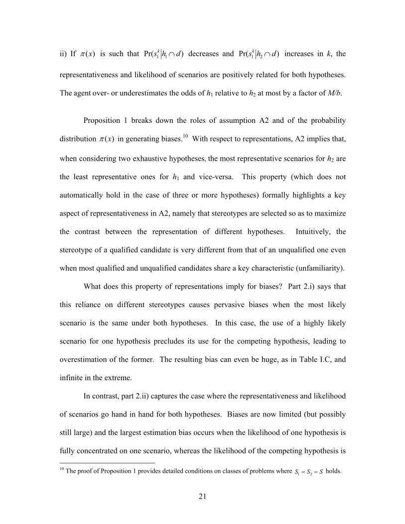
ii) If )(xπ is such that )Pr( 11 dhsk ∩ decreases and )Pr( 21 dhsk ∩ increases in k, the

representativeness and likelihood of scenarios are positively related for both hypotheses.

The agent over- or underestimates the odds of h1 relative to h2 at most by a factor of M/b.

Proposition 1 breaks down the roles of assumption A2 and of the probability

distribution )(xπ in generating biases.10 With respect to representations, A2 implies that,

when considering two exhaustive hypotheses, the most representative scenarios for h2 are

the least representative ones for h1 and vice-versa. This property (which does not

automatically hold in the case of three or more hypotheses) formally highlights a key

aspect of representativeness in A2, namely that stereotypes are selected so as to maximize

the contrast between the representation of different hypotheses. Intuitively, the

stereotype of a qualified candidate is very different from that of an unqualified one even

when most qualified and unqualified candidates share a key characteristic (unfamiliarity).

What does this property of representations imply for biases? Part 2.i) says that

this reliance on different stereotypes causes pervasive biases when the most likely

scenario is the same under both hypotheses. In this case, the use of a highly likely

scenario for one hypothesis precludes its use for the competing hypothesis, leading to

overestimation of the former. The resulting bias can even be huge, as in Table I.C, and

infinite in the extreme.

In contrast, part 2.ii) captures the case where the representativeness and likelihood

of scenarios go hand in hand for both hypotheses. Biases are now limited (but possibly

still large) and the largest estimation bias occurs when the likelihood of one hypothesis is

fully concentrated on one scenario, whereas the likelihood of the competing hypothesis is 10 The proof of Proposition 1 provides detailed conditions on classes of problems where SSS == 21 holds.

22

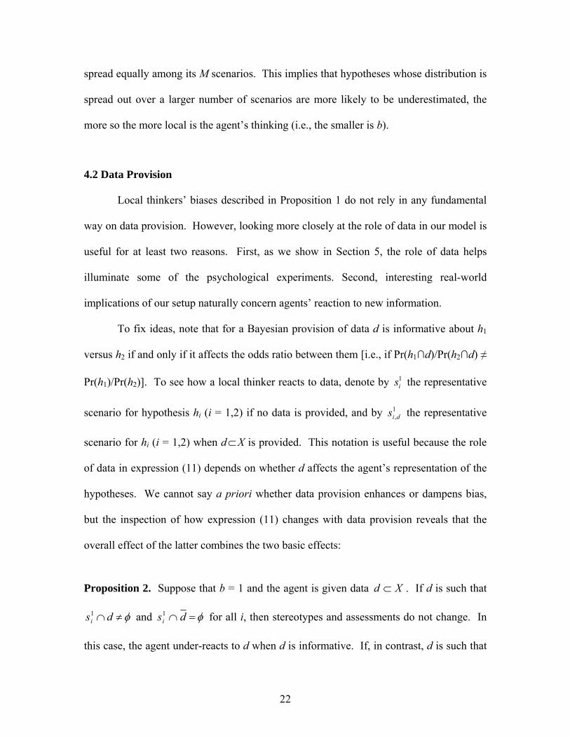
spread equally among its M scenarios. This implies that hypotheses whose distribution is

spread out over a larger number of scenarios are more likely to be underestimated, the

more so the more local is the agent’s thinking (i.e., the smaller is b).

4.2 Data Provision

Local thinkers’ biases described in Proposition 1 do not rely in any fundamental

way on data provision. However, looking more closely at the role of data in our model is

useful for at least two reasons. First, as we show in Section 5, the role of data helps

illuminate some of the psychological experiments. Second, interesting real-world

implications of our setup naturally concern agents’ reaction to new information.

To fix ideas, note that for a Bayesian provision of data d is informative about h1

versus h2 if and only if it affects the odds ratio between them [i.e., if Pr(h1∩d)/Pr(h2∩d) ≠

Pr(h1)/Pr(h2)]. To see how a local thinker reacts to data, denote by 1is the representative

scenario for hypothesis hi (i = 1,2) if no data is provided, and by 1,dis the representative

scenario for hi (i = 1,2) when d⊂X is provided. This notation is useful because the role

of data in expression (11) depends on whether d affects the agent’s representation of the

hypotheses. We cannot say a priori whether data provision enhances or dampens bias,

but the inspection of how expression (11) changes with data provision reveals that the

overall effect of the latter combines the two basic effects:

Proposition 2. Suppose that b = 1 and the agent is given data Xd ⊂ . If d is such that

φ≠∩dsi1 and φ=∩ dsi

1 for all i, then stereotypes and assessments do not change. In

this case, the agent under-reacts to d when d is informative. If, in contrast, d is such that

23

φ=∩ dsi1 for some i, then the stereotype for the corresponding hypothesis must change.

In this case, the agent may over-react to uninformative d.

In the first case, stereotypes do not change with d [i.e. dhshs idiii ∩∩=∩ 1,

1 for

all i], and so data provision affects neither the representation of hypotheses nor -

according to (11) – probabilistic assessments. If the data are informative, this effect

captures the local thinker’s under-reaction because – unlike the Bayesian – the local

thinker does not revise his assessment after observing d.

In the second case, the representations of one or both hypotheses must change

with d. This change can generate over-reaction by inducing the agent to revise his

assessment even when a Bayesian would not do so. This effect increases over-estimation

of 1h if the new representation of 1h triggered by d is relatively more likely than that of

2h [if the bracketed term in (11) rises]. We refer to this effect as data “destroying” the

stereotype of the hypothesis whose representation becomes relatively less likely.

4.3. Conjunction Fallacy

The conjunction fallacy refers to the failure of experimental subjects to follow the

rule that the probability of a conjoined event C&D cannot exceed the probability of event

C or D by itself. For simplicity, we only study the conjunction fallacy when b = 1 and

when the agent is provided no data, but the fundamental logic of the conjunction fallacy

does not rely on these assumptions. We consider the class of problems in (7), but in

Appendix 2 we prove that Proposition 3 holds also for general classes of hypotheses.

24

We focus on the so-called “direct tests”, namely when the agent is asked to

simultaneously assess the probability of a conjoined event h1∩h2 and of one of its

constituent events such as h1. Denote by 12,1s the scenario used to represent the

conjunction h1∩h2 and by 11s the scenario used to represent the constituent event h1. In

this case, the conjunction fallacy obtains in our model if and only if:

)Pr()Pr( 11121

12,1 hshhs ∩≥∩∩ , (13)

i.e., when the probability of the represented conjunction is higher than the probability of

the represented constituent event h1. Expression (13) is a direct consequence of (9), as in

this direct test the denominators are identical and cancel out. The conjunction fallacy

then arises only under the following necessary condition:

Proposition 3. When b = 1, in a direct test of hypotheses h1 and h1∩h2,

)(Pr)(Pr 121 hhh LL ≥∩ only if scenario 11s is not the most likely for 1h .

The conjunction fallacy arises only if the constituent event 1h prompts the use of

an unlikely scenario and thus stereotype. To see why, rewrite (13) as:

)Pr()Pr( 11112

12,1 hshhs ≥∩ . (14)

The conjunction rule is violated when scenario 11s is less likely than 2

12,1 hs ∩ for

hypothesis 1h . Note, though, that 21

2,1 hs ∩ is itself a scenario for 1h since 121

2,1 hhs ∩∩

identifies an element of X. Condition (14) therefore only holds if the representative

scenario 11s is not the most likely scenario for 1h , which proves Proposition 3.11

11 Proposition 3 implies that, if a hypothesis h1 is not represented with the most likely scenario, one can induce the conjunction fallacy by testing h1 against the conjoined hypothesis h1

* = s1*∩ h1, where s1

* is the

25

4.4 Disjunction Fallacy

According to the disjunction rule, the probability attached to an event A should be

equal to the total probability of all events whose union is equal to A. As we discuss in

Section 5.3, however, experimental evidence shows that subjects often under-estimate the

probability of residual hypotheses such as “other” relative to their unpacked version. To

see under what conditions local thinking can account for this fallacy, compare the

assessment of hypothesis h1 with the assessment of hypothesis “h1,1 or h1,2” where

h1,1∪ h1,2 = h1 (and obviously h1,1∩h1,2 = φ ) by an agent with b=1. It is easy to extend

the result to the case where b>1. Formally, we compare PrL(h1) when h1 is tested against

1h with PrL(h1,1) + PrL(h1,2) obtained when the hypothesis “h1,1 or h1,2” is tested against its

complement 1h . The agent then attributes a higher probability to the unpacked version of

the hypothesis, thus violating the disjunction rule, provided PrL(h1,1) + PrL(h1,2) > PrL(h1).

Define 11s , 1

1,1s , 12,1s and 1

0s to be the representative scenarios for hypotheses, 1h ,

1,1h , 2,1h , and 1h respectively. Equation (9) then implies that h1 is underestimated when:

)Pr()Pr()Pr(

)Pr()Pr()Pr()Pr()Pr(

1101

11

111

1102,1

12,11,1

11,1

2,11

2,11,11

1,1

hshshs

hshshshshs

∩+∩∩

>∩+∩+∩

∩+∩. (15)

Equation (15) immediately boils down to:

)Pr()Pr()Pr( 1112,1

12,11,1

11,1 hshshs ∩>∩+∩ , (15’)

meaning that the probability of the representation 111 hs ∩ of 1h is smaller than the sum of

the probabilities of the representations 1,11

1,1 hs ∩ and 2,11

2,1 hs ∩ of 1,1h and 2,1h ,

respectively. Appendix 2 proves that this occurs if the following condition holds:

most likely scenario for h1 and h1

*⊂ h1 is the element obtained by fitting such most likely scenario in hypothesis h1 itself. By construction, in this case PrL(h1

*)≥ PrL(h1), so that the conjunction rule is violated.

26

Proposition 4. Suppose that b = 1. In one test, hypothesis h1 is tested against a set of

alternatives. In another test, the hypothesis “h1,1 or h1,2” is tested against the same set of

alternatives as h1. Then, if s11 is a feasible scenario for either h1,1, h1,2 or both, it follows

that PrL(h1,1) + PrL(h1,2) > PrL(h1) .

Local thinking leads to underestimation of implicit disjunctions. Intuitively,

unpacking a hypothesis h1 into its constituent events reminds the local thinker of

elements of h1 which he would otherwise fail to integrate into his representation. The

sufficient condition for this to occur (that s11 must be a feasible scenario in the explicit

disjunction) is very weak. For example, it is always fulfilled when the representation of

the implicit disjunction s11∩h1 is contained in a sub-residual category of the explicit

disjunction such as “other.”

5. Local Thinking and Heuristics and Biases, with Special Reference to Linda

We now show how our model can rationalize some of the biases in probabilistic

assessments. We cannot rationalize all of the experimental evidence, but rather show that

our model provides a unified account of several findings. At the end of the section, we

discuss the experimental evidence that our model cannot directly explain.

We perform our analysis in a flexible setup based on KT’s (1983) famous Linda

experiment. Subjects are given a description of a young woman, called Linda, who is a

stereotypical leftist, and in particular was a college activist. They are then asked to check

off in order of likelihood the various possibilities of what Linda is today. Subjects

estimate that Linda is more likely to be “a bank teller and a feminist” than merely “a bank

27

teller”, exhibiting the conjunction fallacy. We take advantage of this setup to show how

a local thinker displays a variety of biases, including base rate neglect and the

conjunction fallacy.12 In Section 5.4, we examine the disjunction fallacy experiments.

Suppose that individuals can have one of two possible backgrounds, college

activists (A) and non-activists (NA), be in one of two occupations, bank teller (BT) or

social worker (SW), and hold one of two current beliefs, feminist (F) or non-feminist

(NF). The probability distribution of all possible types is described in tables III.A and B:

A F NF BT

(2/3)(τ/4)

(1/3)(τ/4) SW

(9/10)(2σ/3)

(1/10)(2σ/3)

Table III.A

NA F NF

BT

(1/5)(3τ/4)

(4/5)(3τ/4) SW

(1/2)(σ/3)

(1/2)(σ/3)

Table III.B

Table III.A reports the frequency of activist (A) types, Table III.B the frequency of non-

activist (NA) types. (This full distribution of types is useful to study the effects of

providing data d = A). τ and σ are the base probabilities of a bank teller and a social

worker in the population, respectively, namely Pr(BT) = τ, Pr(SW) = σ.

Table III builds in two main features. First, the majority of college activists are

feminists, while the majority of non-activists are non-feminist, irrespective of their

12 In perhaps the most famous base-rate neglect experiment, KT (1974) gave subjects a personality description of a stereotypical engineer, and told them that he comes from a group of 100 engineers and lawyers, and the share of engineers in the group. In assessing the odds that this person was an engineer or a lawyer, subjects mainly focused on the personality description, barely taking the base-rates of the engineers in the group into account. The parallel between this experiment and the original Linda experiment is sufficiently clear to allow us to analyze base-rate neglect and the conjunction fallacy in the same setting.

28

occupations [Pr(X,F,A) ≥ Pr(X,NF,A) and Pr(X,F,NA) ≤ Pr(X,NF,NA) for X = BT, SW].

Second, social workers are relatively more feminist than bank tellers, irrespective of their

college background (e.g., among activists, 9 out of 10 social workers are feminists while

only 2 out of 3 bank tellers are feminists; among non-activists, half of social workers are

feminists while only 1 out of 5 are non-feminists).

Suppose that a local thinker with b = 1 is told that Linda is a former activist, d =

A, and asked to assess probabilities that Linda is a bank teller (BT), a social worker (SW),

or a feminist bank teller (BT, F). What comes to his mind? Because social workers are

relatively more feminist than bank tellers, the agent represents a bank teller with a “non-

feminist” scenario and a social worker with a “feminist” scenario. Indeed, Pr(BT|A,NF) =

(τ/12)/[(τ/12)+(2σ/30)] > Pr(BT|A,F) = (2τ/12)/[(2τ/12)+(9σ/15)], and Pr(SW|A,NF) <

Pr(SW|A,F). Thus, after the data that Linda was an activist are provided, ‘‘bank teller’’ is

represented by (BT, A, NF), and ‘‘social worker’’ by (SW, A, F). The hypothesis of

“bank teller and feminist” is correctly represented by (BT, A, F) because it leaves no gaps

to be filled. Using equation (11), we can then compute the local thinker’s odds ratios for

various hypotheses, which provide a parsimonious way to study judgement biases.

5.1 Neglect of Base-Rates

Consider the odds ratio between the local thinker’s assessment of “bank teller”

and “social worker”. In the represented state space, this is equal to:

στ

83

10/93/1

),,Pr(),,Pr(

)(Pr)(Pr

⎥⎦⎤

⎢⎣⎡==

FASWNFABT

ASWABT

L

L

. (16)

As in (11), the right-most term in (16) is the Bayesian odds ratio, while the bracketed

term is the ratio of the two representations’ likelihoods. The bracketed term is smaller

29

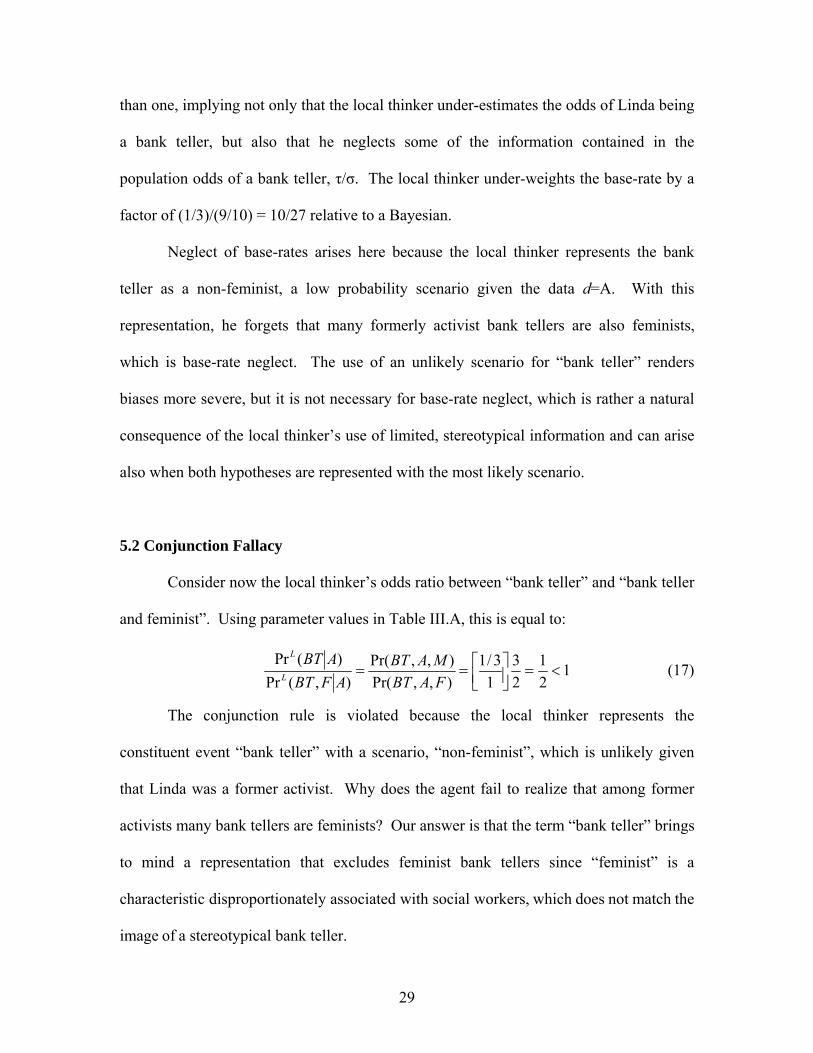
than one, implying not only that the local thinker under-estimates the odds of Linda being

a bank teller, but also that he neglects some of the information contained in the

population odds of a bank teller, τ/σ. The local thinker under-weights the base-rate by a

factor of (1/3)/(9/10) = 10/27 relative to a Bayesian.

Neglect of base-rates arises here because the local thinker represents the bank

teller as a non-feminist, a low probability scenario given the data d=A. With this

representation, he forgets that many formerly activist bank tellers are also feminists,

which is base-rate neglect. The use of an unlikely scenario for “bank teller” renders

biases more severe, but it is not necessary for base-rate neglect, which is rather a natural

consequence of the local thinker’s use of limited, stereotypical information and can arise

also when both hypotheses are represented with the most likely scenario.

5.2 Conjunction Fallacy

Consider now the local thinker’s odds ratio between “bank teller” and “bank teller

and feminist”. Using parameter values in Table III.A, this is equal to:

121

23

13/1

),,Pr(),,Pr(

),(Pr)(Pr

<=⎥⎦⎤

⎢⎣⎡==

FABTMABT

AFBTABT

L

L

(17)

The conjunction rule is violated because the local thinker represents the

constituent event “bank teller” with a scenario, “non-feminist”, which is unlikely given

that Linda was a former activist. Why does the agent fail to realize that among former

activists many bank tellers are feminists? Our answer is that the term “bank teller” brings

to mind a representation that excludes feminist bank tellers since “feminist” is a

characteristic disproportionately associated with social workers, which does not match the

image of a stereotypical bank teller.

30

One alternative explanation of the conjunction fallacy discussed in KT (1983)

holds that the subjects substitute the target assessment of Pr(h|d) with that of Pr(d|h).13 In

our Linda example, this error can indeed yield the conjunction fallacy because Pr(A|BT) =

1/4 < Pr(A|F,BT) = 10/19. Intuitively, being feminist (on top of being bank teller) can

increase the chance of being Linda. KT (1983) addressed this possibility in some

experiments. In one of them, subjects were told that the tennis player Bjorn Borg had

reached the Wimbledon final, and then asked to assess whether it was more likely that in

the final Borg would lose the first set or whether he would lose the first set but win the

match. Most subjects violated the conjunction rule by stating that the second outcome

was more likely than the first. As we show in Appendix 3 using a model calibrated with

actual data, our approach can explain this evidence, but a mechanical assessment of

Pr(d|h) cannot. The reason, as KT point out, is that Pr(Borg has reached the final| Borg’s

score in the final) is always equal to one, regardless of the final score.

Most important, the conjunction fallacy explanation based on the substitution of

Pr(h|d) with Pr(d|h) relies on the provision of data d. This story cannot thus explain the

conjunction rule violations that occur in the absence of data provision. To see how our

model can account for those, consider another experiment from KT (1983). Subjects are

asked to compare the likelihoods of “A massive flood somewhere in North America in

which more than 1000 people drown” to that of “An earthquake in California causing a

flood in which more than 1000 people drown.” Most subjects find the latter event, which

is a special case of the former, to be nonetheless more likely.

13 In a personal communication, Xavier Gabaix proposed a “local prime” model complementary to our local thinking model. Such a model exploits the above intuition about the conjunction fallacy. Specifically, in the local prime model an agent assessing h1, …, hn evaluates PrL’(hi|d) = Pr(d|hi)/[ Pr(h1|d) + …+ Pr(hn|d)].

31

We discuss this example formally in Appendix 3, but the intuition is

straightforward. When earthquakes are not mentioned, massive floods are represented by

an unlikely scenario of disastrous storms, as storms are a stereotypical cause of floods. In

contrast, when earthquakes in California are explicitly mentioned, the local thinker

realizes that these can cause much more disastrous floods, changes his representation, and

attaches a higher probability to the outcome because earthquakes in California are quite

common. This example vividly illustrates the key point that it is the hypothesis itself,

rather than the data, than frames both the representation and the assessment.

The general idea behind these types of conjunction fallacy is that either the data

(Linda is a former activist) or the question itself (floods in North America) bring to mind

a representative but unlikely scenario. This general principle can help explain other

conjunction rule violations. For example, Kahneman and Frederick (2005) report that

subjects estimate the annual number of murders in the state of Michigan to be lower than

that in the city of Detroit, which is in Michigan. Our model suggests that this might be

explained by the fact that the stereotypical location in Michigan is rural and non-violent,

so subjects forget that the more violent city of Detroit is in the state of Michigan as well.

5.3 The Role of Data and Insensitivity to Predictability

Although base rates neglect and the conjunction fallacy do not rely on data

provision, previous results illustrate the effects of data in our model. Suppose that a local

thinker assesses the probabilities of bank teller, social worker, and feminist bank teller

before being given any data. From Table III.B, “social worker” is still represented by

(SW, A, F) and “bank teller and feminist” by (BT, A, F). Crucially, however, “bank

32

teller” is now represented by (BT, NA, NF). This is the only representation that changes

after d = A is provided. Before data are provided, then, we have:

στ

στ

65

)3/2)(10/9()8/6)(3/2(

),,Pr(),,Pr(

)(Pr)(Pr

===FASWMNABT

SWBT

L

L

, (18)

15

181960

19/105/3

),,Pr(),,Pr(

),(Pr)(Pr

>=⎥⎦⎤

⎢⎣⎡==

FABTMNABT

FBTBT

L

L

. (19)

Biases now are either small or outright absent. Expression (18) gives an almost

correct unconditional probability assessment for the population odds ratio of τ/σ. In

expression (19), not only does the conjunction rule hold, but the odds of “bank teller” are

overestimated. So what happens when data are provided?

As in Proposition 2, this is a case where data provision “destroys” the stereotype

of only one of the hypotheses, “bank teller.” Before Linda’s college career is described, a

bank teller is “non activist, non-feminist.” This stereotype is very likely. However, after

d = A is provided, the representation of “bank teller” becomes an unlikely one, because

even for bank tellers it is extremely unlikely to have become “non feminist” after having

been “activist”. The probability of Linda being a bank teller is thus underestimated,

generating both severe base-rates neglect and the conjunction fallacy.

This analysis illustrates the role of data not only in the Linda setup but also in the

electoral campaign example. In both cases, the agent is given a piece of data (d = A or d

= drink milk with hotdog) that is very informative about an attribute defining stereotypes

(political orientation or familiarity). By changing the likelihood of the stereotype such

data induce drastic updating, even when the data themselves are scarcely informative

about the target assessment (occupation or qualification).

33

This over-reaction to scarcely informative data provides a rationalization for the

“insensitivity to predictability” displayed by experimental subjects. We formally show

this point in Appendix 3 based on a famous KT experiment on practice talks.

In sum, a local thinker’s use of stereotypes provides a unified explanation for

several KT biases. To account for other biases, we need to move beyond the logic of

representativeness as defined here. For instance, our model cannot directly reproduce the

Cascells, Schoenberger, and Graboys (1978) evidence on physicians’ interpretation of

clinical tests or the blue versus green cab experiment (KT 1982). KT themselves (1982,

p. 154) explain why these biases cannot be directly attributed to representativeness. We

do not exclude the possibility that these biases are a product of local thinking, but

progress in understanding different recall processes is needed to establish the connection.

5.4. Disjunction and Car Mechanics Revisited.

Fischhoff, Slovic and Lichtenstein (1978) document the violation of the

disjunction rule experimentally. They asked car mechanics, as well as lay people, to

estimate the probabilities of different causes of a car’s failure to start. They document

that on average the probability assigned to the residual hypothesis – “The cause of failure

is something other than the battery, fuel system, or the engine” – went up from 0.22 to

0.44 when that hypothesis was broken up into more specific causes (e.g., the starting

system, the ignition system). Respondents, including experienced car mechanics,

discounted hypotheses that were not explicitly mentioned. The under-estimation of

implicit disjunctions has been documented in many other experiments and is the key

assumption behind Tversky and Koehler’s (1994) support theory.

34

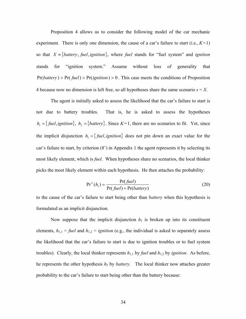
Proposition 4 allows us to consider the following model of the car mechanic

experiment. There is only one dimension, the cause of a car’s failure to start (i.e., K = 1)

so that { }ignitionfuelbatteryX ,,≡ , where fuel stands for “fuel system” and ignition

stands for “ignition system.” Assume without loss of generality that

0)Pr()Pr()Pr( >>> ignitionfuelbattery . This case meets the conditions of Proposition

4 because now no dimension is left free, so all hypotheses share the same scenario s = X.

The agent is initially asked to assess the likelihood that the car’s failure to start is

not due to battery troubles. That is, he is asked to assess the hypotheses

{ }ignitionfuelh ,1 = , { }batteryh =2 . Since K = 1, there are no scenarios to fit. Yet, since

the implicit disjunction { }ignitionfuelh ,1 = does not pin down an exact value for the

car’s failure to start, by criterion (8’) in Appendix 1 the agent represents it by selecting its

most likely element, which is fuel. When hypotheses share no scenarios, the local thinker

picks the most likely element within each hypothesis. He then attaches the probability:

)Pr()Pr()Pr()(Pr 1 batteryfuel

fuelhL

+= (20)

to the cause of the car’s failure to start being other than battery when this hypothesis is

formulated as an implicit disjunction.

Now suppose that the implicit disjunction h1 is broken up into its constituent

elements, h1,1 = fuel and h1,2 = ignition (e.g., the individual is asked to separately assess

the likelihood that the car’s failure to start is due to ignition troubles or to fuel system

troubles). Clearly, the local thinker represents h1,1 by fuel and h1,2 by ignition. As before,

he represents the other hypothesis h2 by battery. The local thinker now attaches greater

probability to the car’s failure to start being other than the battery because:

35

)Pr()Pr()Pr()(Pr

)Pr()Pr()Pr()Pr()Pr()(Pr)(Pr

1 batteryfuelfuelh

batteryfuelignitionfuelignitionfuelignition

L

LL

+=>

+++

=+. (21)

In other words, we can account for the observed disjunction fallacy. The logic is the

same as that of Proposition 4: the representation of the explicit disjunction adds to the

representation of the implicit disjunction (x = fuel) an additional element (x = ignition),

which boosts the assessed probability of the explicit disjunction.

6. An Application to Demand for Insurance

Buying insurance is supposed to be one of the most compelling manifestations of

economic rationality, in which risk-averse individuals hedge their risks. Yet both

experimental and field evidence, summarized by Cutler and Zeckhauser (2004) and

Kunreuther and Pauly (2005), reveal some striking anomalies in individual demand for

insurance. Most famously, individuals vastly overpay for insurance against narrow low

probability risks, such as those of airplanes crashing or appliances breaking. They do so

especially after the risk is brought to their attention, but not when risks remain

unmentioned. In a similar vein, people prefer insurance policies with low deductibles,

even when the incremental cost of insuring small losses is very high (Johnson et al. 1993,

Sydnor 2006). Meanwhile, Johnson et al. (1993) present experimental evidence that

individuals are willing to pay more for insurance policies that specify in detail the events

being insured against than they do for policies insuring “all causes.”

Our model, particularly the analysis of the disjunction fallacy, may shed light on

this evidence. Suppose that an agent with a concave utility function u(.) faces a random

wealth stream due to probabilistic realizations of various accidents. For simplicity, we

36

assume that at most one accident occurs. There are three contingencies s = 0, 1, 2, each

occurring with an ex-ante probability πs. Contingency s = 0 is the status quo or no loss

contingency. In this state, the agent’s wealth is at its baseline level 0w . Contingencies 1

and 2 correspond to the realizations of distinct accidents, which entail wealth levels

0wws < for s = 1, 2. A contingency s = 1,2 then represents the income loss caused by a

car accident, a specific reason for hospitalization, or a plane crash from a terrorist attack.

We assume that π0 > max(π1, π2), so that the status quo is the most likely event.

We first show that a local thinker in this framework exhibits behaviour consistent

with Johnson et al.’s (1993) experiments. The authors find, for example, that, in plane

crash insurance, subjects are willing to pay more in total for insurance against a crash

caused by “any act of terrorism” plus insurance against a crash caused by “any non-

terrorism related mechanical failure” than for insurance against a crash for “any reason”

(p. 39). Likewise, subjects are willing to pay more in total for insurance policies paying

for hospitalization costs in the events of “any disease” and “any accident” than for a

policy that pays those costs in the event of hospitalization for “any reason” (p. 40).

As a starting point, note that the maximum amount P that a rational thinker is

willing to pay to insure his status quo income against “any risks” is given by

u[w0 – P] = E[u(w)]. (22)

The rational thinker would pay the same amount P for insurance against any risk as for

insurance against either s =1 or s = 2 occurring, since he keeps all the outcomes in mind.

Suppose now that a local thinker of order one (b = 1) considers the maximum

price he is willing to pay to insure against any risk (i.e., against the event s ≠ 0). For a

local thinker, only one (representative) risk comes to mind. Suppose without loss of

37

generality that π1 > π2. Then, just as in the car mechanic example, only the more likely

event s = 1 comes to the local thinker’s mind. As a consequence, he is willing to pay up

to LP for coverage against any risk, defined by:

u[w0 – PL] = E[u(w)| s = 0, 1] . (23)

The local thinker’s maximum willingness to pay directly derives from his certainty

equivalent wealth conditional on the state belonging to the event “s = 0 or 1”. If, in

contrast, the local thinker is explicitly asked to state the maximum willingness to pay for

insuring against either s = 1, 2 occurring, then both events come to mind and his

maximum price is identical to the rational thinker’s price of P.

Putting these observations together, it is easy to show that the local thinker is

willing to pay more for the unpacked coverage whenever:

u(w2) ≤ E[u(w)| s = 0, 1] (24)

That is, condition (24) and thus the Johnson et al. (1993) experimental findings would be

confirmed when, as in the experiments, the two events entail identical losses so that

21 ww = (plane crash due to one of two possible causes). In this case, insurance against s

= 2 is valuable, and therefore the local thinker is willing to pay less for coverage against

“any accident” than when all the accidents are listed because, in the former case, he does

not recall s = 2. This partial representation of accidents leads the agent to under-estimate

his demand for insurance relative to the case in which all accidents are spelled out.

The same logic illuminates over-insurance against specific risks, such as a broken

appliance or small property damage, as documented by Cutler and Zeckhauser (2004) and

Sydnor (2006). A local thinker would in fact pay more for insurance against a specific

38

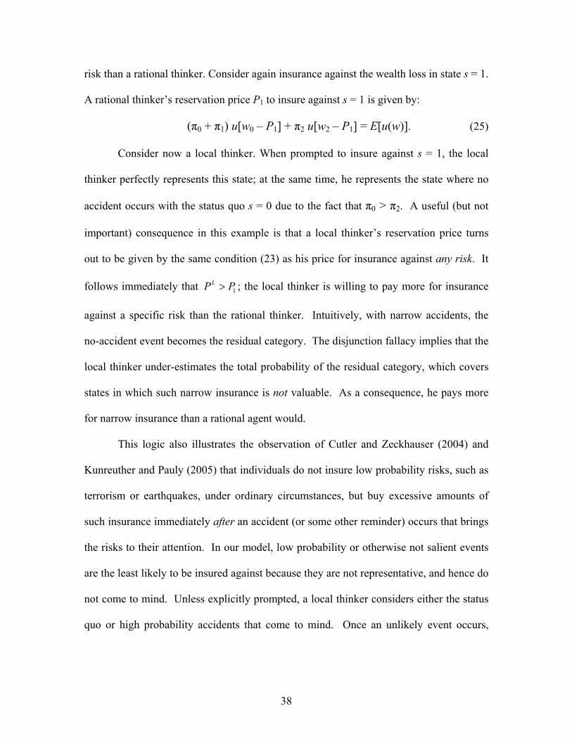
risk than a rational thinker. Consider again insurance against the wealth loss in state s = 1.

A rational thinker’s reservation price P1 to insure against s = 1 is given by:

(π0 + π1) u[w0 – P1] + π2 u[w2 – P1] = E[u(w)]. (25)

Consider now a local thinker. When prompted to insure against s = 1, the local

thinker perfectly represents this state; at the same time, he represents the state where no

accident occurs with the status quo s = 0 due to the fact that π0 > π2. A useful (but not

important) consequence in this example is that a local thinker’s reservation price turns

out to be given by the same condition (23) as his price for insurance against any risk. It

follows immediately that 1LP P> ; the local thinker is willing to pay more for insurance

against a specific risk than the rational thinker. Intuitively, with narrow accidents, the

no-accident event becomes the residual category. The disjunction fallacy implies that the

local thinker under-estimates the total probability of the residual category, which covers

states in which such narrow insurance is not valuable. As a consequence, he pays more

for narrow insurance than a rational agent would.

This logic also illustrates the observation of Cutler and Zeckhauser (2004) and

Kunreuther and Pauly (2005) that individuals do not insure low probability risks, such as

terrorism or earthquakes, under ordinary circumstances, but buy excessive amounts of

such insurance immediately after an accident (or some other reminder) occurs that brings

the risks to their attention. In our model, low probability or otherwise not salient events

are the least likely to be insured against because they are not representative, and hence do

not come to mind. Unless explicitly prompted, a local thinker considers either the status

quo or high probability accidents that come to mind. Once an unlikely event occurs,

39

however, or is explicitly brought to the local thinker’s attention, it becomes part of the

representation of risky outcomes and is over-insured.

Local thinking can thus provide a unified explanation of two anomalous aspects

of demand for insurance: over-insurance against narrow and well-defined risks, as well as

underinsurance against broad or vaguely defined risks. The model might also help

explain other insurance anomalies, such as the demand for life insurance rather than for

annuities by the elderly parents of well-off children (Cutler and Zeckhauser 2004). We

leave a discussion of these issues to future work.

7. Conclusion

We have presented a simple model of intuitive judgment in which the agent

receives some data and combines it with information retrieved from memory to evaluate

a hypothesis. The central assumption of the model is that, in the first instance,

information retrieval from memory is both limited and selective. Some, but not all, of the

missing scenarios come to mind. Moreover, what primes the selective retrieval of

scenarios from memory is the hypothesis itself, with scenarios most predictive of that

hypothesis – the representative scenarios -- being retrieved first. In many situations, such

intuitive judgment works well, and does not lead to large biases in probability

assessments. But in situations where the representativeness and likelihood of scenarios

diverge, intuitive judgment becomes faulty. We showed that this simple model accounts

for a significant number of experimental results, most of which are related to the

representativeness heuristic. In particular, the model can explain the conjunction and

40

disjunction fallacies exhibited by experimental subjects. The model also sheds light on

some puzzling evidence concerning demand for insurance.

To explain the evidence, we took a narrow view of how recall of various

scenarios takes place. In reality, many other factors affect recall. Both availability and

anchoring heuristics described by Kahneman and Tversky (1974) bear on how scenarios

come to mind, but through mechanisms other than those we elaborated.

At a more general level, our model relates to the distinction, emphasized by

Kahneman (2003), between System 1 (quick and intuitive) and system 2 (reasoned and

deliberate) thinking. Local thinking can be thought of as a formal model of System 1.

However, from our perspective, intuition and reasoning are not so radically different.

Rather, they differ in what is retrieved from memory to make an evaluation. In the case

of intuition, the retrieval is not only quick, but also partial and selective. In the case of

reasoning of the sort studied by economists, retrieval is complete.

Indeed, in economic models, we typically think of people receiving limited

information from the outside world, but then combining it with everything they know to

make evaluations and decisions. The point of our model is that, at least in making quick

decisions, people do not bring everything they know to bear on their thinking. Only

some information is automatically recalled from passive memory, and – crucially to

understanding the world – the things that are recalled might not even be the most useful.

Heuristics, then, are not limited decisions. They are decisions like all the others, but

based on limited and selected inputs from memory. System 1 and System 2 are examples

of the same mode of thought; they differ in what comes to mind.

Universitat Pompeu Fabra, CREI, CEPR and Harvard University

41

Appendix 1: Local thinking with general hypotheses and data

Hypotheses and data may constrain some dimensions of the state space X without restricting them to particular values, as we assumed in (7). Generally:

{ }ii HxXxdh ∈∈≡∩ , for some Ii∈ (7’)

where { }KI ,...,1⊆ is the set of dimensions constrained by dh∩ , and ii XH ⊂ are the sets they specify for each Ii∈ . Dimensions Ii∉ are left free. The class of hypotheses in (7) is a special case of that in (7’) when the sets Hi are singletons.

To generalize the definition of representation of a hypothesis, we assume that agents follow a three stage procedure. First, each hypothesis dh∩ is decomposed into all of its constituent “elementary hypotheses”, defined as those that fix one exact value for each dimension in I. For each elementary hypothesis, agents then consider all possible scenarios, according to Definition 1. Finally, agents order the set of elementary hypotheses together with the respective feasible scenarios according to their conditional probabilities.14 An agent with b = 1 would simply solve:

[ ]dsxIsxI

∩Prmax,

, (8’)

where { }iiI xxXxx ˆ: =∈≡ where ii Hx ∈ˆ , Ii∈∀ . Thus, conditional on fixing Ix , scenario s is the exact equivalent of the scenario in Definition 1. A solution to problem (8’) always exists due to finiteness of the problem.

This procedure generates a representation dxs rIr ∩∩ 1,

1 for hypothesis rh which

is the general counterpart of the representation dhs rr ∩∩1 used in the class of problems

in (7). Accordingly, (8’) yields a ranking of all possible representations krI

kr xs ,∩ of rh

that in turn ranks all elements in dhr ∩ in terms of their order of recall. Formula (9) can now be directly applied to calculate the local thinker’s probabilistic assessment. In the case of exhaustive hypotheses in the general class (7’), that assessment can be written as:

∑ ∑

∑

= =

=

∩⎥⎦

⎤⎢⎣

⎡∩∩

∩⎥⎦

⎤⎢⎣

⎡∩∩

=N

rr

b

kr

krI

kr

t

b

kt

ktI

kt

tL

dhdhxs

dhdhxsdh

1 1,

1,

)Pr()Pr(

)Pr()Pr()(Pr (9’’)

Expression (9’’) is an immediate generalization of (9’). Except for Proposition 1, which is proved only for problems in (7), all the results in the paper generalize to hypotheses of

14 This assumption captures the idea that dimensions explicitly mentioned in the hypothesis are selected to maximize the probability of the latter. We could assume that filling gaps in hypotheses taking form (7’) is equivalent to selecting scenarios, in the sense that the agent maximizes (8) subject to scenarios dhs ∩∈ . Our main results would still hold in this case, but all scenarios dhs r ∩∈ would be equally representative, as expression (8) would always be equal to 1. Assumption (8’) captures the intuitive idea that the agent also orders the representativeness of elements belonging to ranges explicitly mentioned in the hypothesis itself.

42

type (7’). The only caveat that in this case element dhs rkr ∩∩ should be read as the

intersection of the set of specific values chosen by the agent for representing rh with the

data and the chosen scenario, i.e. as dxs krI

kr ∩∩ , , which is the k’th ranked term

according to objective (8’). Appendix 2: Proofs Proof of Proposition 1. Proposition 1 is restricted to the case where hypotheses 1h and

2h belong to class (7). Note first that any finite state space can be represented as

{ }KX 1,0= generated by the product of K binary dimensions. We assume that K>2 to allow for hypotheses, data and scenarios. If 1h and 2h have the same set of feasible scenarios ( 21 SS = ) then they necessarily fix the same set of dimensions ( 21 II = ). Since

dimensions are binary, it follows that 12 hh = . For simplicity, focus on the class of problems where: i) the hypotheses 1h , 2h fix the value of only one dimension and ii) the data d fix the value of N-1 other dimensions, N<K. The condition SSS == 21 still holds.

To prove claim 1), apply Definition 1 and Assumption A2 to find that the representativeness of Ss∈ for 1h is equal to

[ ])Pr()Pr(/)Pr()Pr( 2111 sdhsdhsdhdsh ∩∩+∩∩∩∩=∩ . The representativeness of

Ss∈ for 2h is equal to )Pr(1)Pr( 12 dshdsh ∩−=∩ . The representativeness of

scenarios for the two hypotheses is thus perfectly inversely related, formally 121

+−= kMk ss for k = 1,…,M.

Consider now claim 2.i). For any b < M, 1h is represented with scenarios { } bkks ≤1 ,

while 2h is represented with { } bkkMs ≤

−+11 . From (9), the odds of 1h are (weakly) over-

estimated if and only if:

∑∑=

−+

=

∩≥∩b

k

kMb

k

k dhsdhs1

21

11

11 )Pr()Pr(

Suppose that )Pr( 11 dhs k ∩ and )Pr( 21 dhs k ∩ strictly decrease in k. It then follows that

the above condition is met for every b < M. To establish a contradiction, suppose that for a certain b* < M the above condition is not met, that is

∑∑=

−+

=

∩<∩**

12

11

111 )Pr()Pr(

b

k

kMb

k

k dhsdhs (26)

Then, for some b** ≤ b* , it must be the case that )Pr()Pr( 21

111****

dhsdhs bMb ∩<∩ −+ .

But since )Pr( 11 dhs k ∩ and )Pr( 21 dhs k ∩ are strictly decreasing in k, it must also be the

case that )Pr()Pr( 21

111 dhsdhs bMb ∩<∩ −+ for all b > b*. This implies that (26) holds for

all b > b*, including b = M, but this is inconsistent with the fact that

43

1)Pr()Pr(1

21

11

11 =∩=∩ ∑∑=

−+

=

M

k

kMM

k

k dhsdhs .

The same logic allows us to show that if )Pr( 11 dhs k ∩ and )Pr( 21 dhs k ∩ are strictly

increasing in k, the odds of 1h are (weakly) underestimated for any b<M. To see how in the first case the overestimation of 1h may be infinite, consider a

probability distribution )(xπ such that:

)1(22

2

111 11)Pr()Pr( −

−−

∩=∩∩ kM

k dhdhs εεε , )1(

221 11)Pr()Pr( −

−−

∩=∩∩ kM

k dhdhs εεε

for all k≥1, where 0 < ε < 1. Then, for all b ≤ M, we have that:

M

bb

k

k dhs 2

2

111 1

1)Pr(εε

−−

=∩∑=

, M

MbMb

k

kM dhsεεε

−−

=∩−

=

−+∑ 1)Pr(

12

11

Inserting these expressions into (11), we see that as ε → 0 the extent of overestimation becomes arbitrarily large for any b < M.

Finally, to prove claim 2.ii), recall that 1h and 2h are represented with scenarios 11s and Ms1 respectively. If )(xπ is such that )Pr( 11 dhsk ∩ decreases and )Pr( 21 dhs k ∩

increases in k, the two hypotheses are represented with their most likely scenarios. Thus, the greatest overestimation of 1h relative to 2h is reached when 1h is concentrated on its most likely scenario while the distribution of 2h is fully dispersed among all scenarios,

that is 1)Pr( 111 =∩ dhs and Mdhs M /1)Pr( 21 =∩ . In this case, the agent overestimates

the odds of 1h by a factor of bMMb

k//1

1

1=⎟

⎠

⎞⎜⎝

⎛−

=∑ .

Proof of Proposition 2. To prove the proposition, we explicitly focus on hypotheses of the form in (7), but all of the results are easily extended to the case where hypotheses take the general form (7’) by simply substituting hi with k

iIx , when scenario kis is used. The

central part of the argument amounts to proving that if φ≠∩dsi1 and φ=∩ dsi

1 for all

i, then stereotypes do not change. Formally, dhshs idiii ∩∩=∩ 1,

1 for all i, where 1,dis is

the most representative scenario after data d is provided. We prove this property by contradiction. If dhshs idiii ∩∩≠∩ 1

,1 for some i, then it must also be the case that

dss dii ∩≠ 1,

1 and therefore

)Pr()Pr(

)Pr()Pr(

)Pr()Pr(

1,

1,

1

1

1

1

dshdsh

dshdsh

shsh

dii

dii

ii

ii

ii

ii

∩∩

∩∩<

∩∩∩∩

=∩∩

. (27)

44

Condition (27) follows from three considerations. First, since φ≠∩dsi1 and

φ=∩ dsi1 for all i, we have that )Pr()Pr( 11 dshsh iiii ∩∩=∩ , which implies the

equality on the left hand side in (27). Second, since φ≠∩dsi1 , then dsi ∩

1 contains a

scenario for dhi ∩ [this scenario is identified by the sub-vector s of elements in 1is not

fully pinned down by d]. This is because dhs ii ∩∩1 identifies an element in X. Third,

the scenario s identified in dsi ∩1 must be less representative than 1

,dis because the latter

is defined as the most representative scenario for dhi ∩ . But then, since ds di ∩1, is also

a scenario for ih , the relationship between the first and third terms in condition (27)

contradicts the fact that 1is is the most representative scenario for ih . This proves that

dhshs idiii ∩∩=∩ 1,

1 , which directly implies that assessments do not change, upon

provision of d, even if d is informative. If, in contrast, φ=∩ dsi1 for some i, then the

stereotype for the corresponding hypothesis must change. Then assessments can change even if the data is barely informative, as Section 5.3 and Appendix 3.A show. Here we show that the local thinker may even react to completely uninformative data. Consider the example below:

Data = d1 s1 s2

h1 ε1 π1 - ε1

h2 0 π2

Data = d2 s1 s2

h1 0 π1

h2 ε2 π2- ε2

The tables represent the distribution π(x) on hypotheses h1 and h2 such that the

data d1, d2 are completely uninformative (and ε1, ε2 are small positive numbers). When no data is provided, the local thinker represents h1 with (s1, d1) and h2 with (s1, d2), assessing PrL(h1) = ε1/(ε1 + ε2). After for instance d1 is provided, the representation for h1 does not change but the one for h2 switches to (s2, d1). As a result, PrL(h1|d1) = ε1/(ε1 + π 2) << PrL(h1) even if the data is completely uninformative. This example is obviously extreme, but it gives an idea of the forces towards over-reaction in our model. Generalization of Proposition 3 to the Class of Problems in (7’). Since b=1, each hypothesis ih is represented by 11

, iiI sxi∩ , where 11

, , iiI sxi

satisfy (8’). Then condition (13)

translates directly into )Pr()Pr( 11,

11

12,

11,

12,1 121 III xsxxs ∩≥∩∩ . Since both elements for

which probabilities are computed in this condition are representations of 1h , we can

45

rewrite this as )Pr()Pr( 11

1,111

11,

12,

12,1 112

hxshxxs III ∩≥∩∩ . This in turn implies that

representation 11,

12,1 1I

xs ∩ must not be the most likely one for 1h , since 12,

11,

12,1 21 II xxs ∩∩ is

itself a more likely representation for 1h . Proof of Proposition 4. We assume the implicit disjunction hypothesis 2,11,11 hhh ∪=

specifies a range of values, as this more general setting simplifies the analysis of the car mechanic experiment. In condition (15), the expression rr hs ∩1 should be read as

)( 11Irr xhs ∩ where )( 1

Ir xh and 1rs satisfy (8’). Note that representations follow a

“revealed preference” logic: if the local thinker represents 1h with { }11

1 , sxI , then he will

always use the same representation for any hypothesis 10 hh ⊂ as long as 01 hxI ∈ and 1

1s

is a feasible scenario for 0h , in the sense that 0h and 1h constrain the same set of

dimensions I. To see this, suppose that the representation of 0h is equal to some other

element { }*0

* , sxI , so that:

( ) ( )dsxdsx II ∩>∩ 11

1*0

* PrPr .

But this leads to a contradiction, since { }*0

* , sxI would then be a representation of 1h with

higher conditional probability (8’) than { }11

1 , sxI . Continuing the proof, recall that by

assumption 11s is a scenario for either 1,1h or 2,1h , or both. Therefore, { }1

11 , sxI is the

representation of the hypotheses for which 11s is a scenario. As a result, condition (15)

holds and the disjunction fallacy follows. Appendix 3 (for the Web). Additional Experiments A. Insensitivity to Predictability

KT (1974) presented subjects with descriptions of the performance of a student-teacher during a particular practice lesson. Some subjects were asked to evaluate the quality of the lesson, other subjects were asked to predict the standing of the student-teacher five years after the practice lesson. The judgments made under the two conditions were identical, irrespective of subjects’ awareness of the limited predictability of teaching competence five years later on the basis of a single trial lesson.

To explore the consequences of local thinking on insensitivity to predictability, consider a local thinker who assesses the quality of a candidate based on the latter’s job talk at a university department. The state space has three dimensions: the candidate’ quality, which can be high (H) or low (L), the quality of his talk, which can be good (GT) or bad (BT), and his expressive ability, which can be articulate (A) or inarticulate (I). The distribution of these characteristics is as follows:

46

Good Talk (GT) Inarticulate (I) Articulate (A) High Quality (H) 0.005 0.25Low Quality (L) 0.005 0.24

Table A.1

Bad Talk (BT) Inarticulate (I) Articulate (A)High Quality (H) 0.24 0.005Low Quality (L) 0.25 0.005

Table A.2

In tables A.1 and A.2, the quality of the talk is highly correlated with expressive ability, but the latter dimension is only barely informative of the candidate’s quality. Still, the candidate’s expressive ability is always representative of his quality, i.e. after listening to the talk the local thinker represents low quality candidates as inarticulate, and high quality ones as articulate. The tables are admittedly extreme, but they illustrate the point in the starkest manner. The local thinker then assesses:

02.0),,Pr(),,Pr(

)(Pr)(Pr

50),,Pr(),,Pr(

)(Pr)(Pr

==

==

IBTLABTH

BTLBTH

IGTLAGTH

GTLGTH

L

L

L

L

The local thinker grossly over-estimates the quality of the candidate after a good talk and under-estimates it after a bad talk. Indeed, in this example a Bayesian would estimate Pr(H|GT)/Pr(L|GT) = 1.04 and Pr(H|BT)/Pr(L|BT) = 0.96 !!

Over-reaction here is due to the fact that the data (quality of the talk) are scarcely informative about the target attribute (quality of the candidate), but very informative about an attribute defining the stereotype for different hypotheses (expressive ability). As in the Linda example, Tables A.1 and A.2 exploit the divergence between representativeness and likelihood to illustrate this phenomenon in the starkest manner, but over-reaction to data is a natural and general consequence of the use of stereotypes. B. Conjunction Fallacy in the Bjorn Borg Experiment

Suppose that a local thinker is given d = “Bjorn Borg is in the Wimbledon Final” and asked to assess Pr(Borg wins 1st set), Pr(Borg loses 1st set), Pr(Borg loses 1st and wins the match). The first hypothesis ensures exhaustivity, but it is not necessary to obtain the result. When prompted to assess these hypotheses, the agent fits an overall evaluation of Borg’s game which can take two values: Borg loses the match (LM), Borg wins the match (WM). Suppose that the distribution of these characteristics is as follows:

Borg is in Wimbledon Final Loses the Match (LM) Wins the Match (WM) Loses First Set (LS) 3/16 4/16 Wins First Set (WS) 2/16 7/16

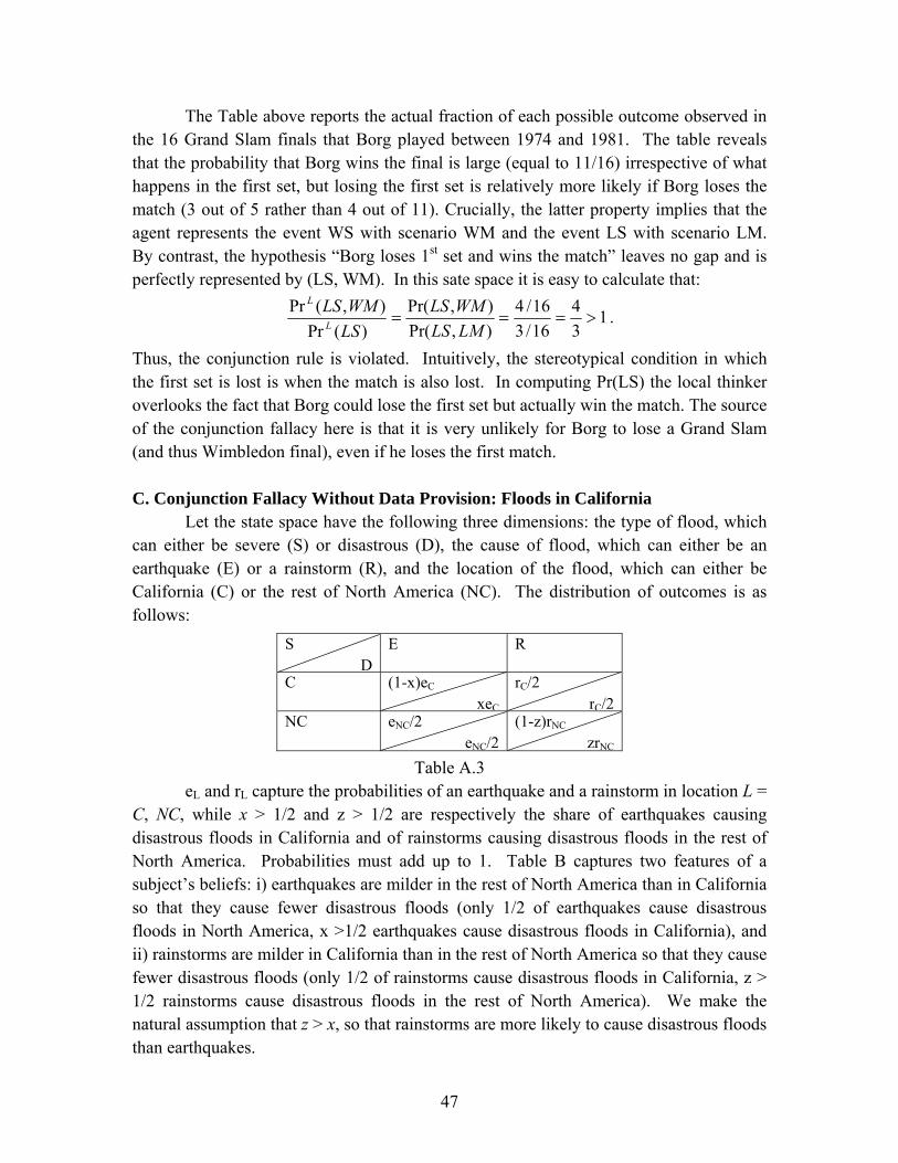
47

The Table above reports the actual fraction of each possible outcome observed in the 16 Grand Slam finals that Borg played between 1974 and 1981. The table reveals that the probability that Borg wins the final is large (equal to 11/16) irrespective of what happens in the first set, but losing the first set is relatively more likely if Borg loses the match (3 out of 5 rather than 4 out of 11). Crucially, the latter property implies that the agent represents the event WS with scenario WM and the event LS with scenario LM. By contrast, the hypothesis “Borg loses 1st set and wins the match” leaves no gap and is perfectly represented by (LS, WM). In this sate space it is easy to calculate that:

134

16/316/4

),Pr(),Pr(

)(Pr),(Pr

>===LMLSWMLS

LSWMLS

L

L

.

Thus, the conjunction rule is violated. Intuitively, the stereotypical condition in which the first set is lost is when the match is also lost. In computing Pr(LS) the local thinker overlooks the fact that Borg could lose the first set but actually win the match. The source of the conjunction fallacy here is that it is very unlikely for Borg to lose a Grand Slam (and thus Wimbledon final), even if he loses the first match. C. Conjunction Fallacy Without Data Provision: Floods in California

Let the state space have the following three dimensions: the type of flood, which can either be severe (S) or disastrous (D), the cause of flood, which can either be an earthquake (E) or a rainstorm (R), and the location of the flood, which can either be California (C) or the rest of North America (NC). The distribution of outcomes is as follows:

S D

E R

C (1-x)eC

xeC

rC/2rC/2

NC eNC/2eNC/2

(1-z)rNC

zrNC

Table A.3 eL and rL capture the probabilities of an earthquake and a rainstorm in location L =

C, NC, while x > 1/2 and z > 1/2 are respectively the share of earthquakes causing disastrous floods in California and of rainstorms causing disastrous floods in the rest of North America. Probabilities must add up to 1. Table B captures two features of a subject’s beliefs: i) earthquakes are milder in the rest of North America than in California so that they cause fewer disastrous floods (only 1/2 of earthquakes cause disastrous floods in North America, x >1/2 earthquakes cause disastrous floods in California), and ii) rainstorms are milder in California than in the rest of North America so that they cause fewer disastrous floods (only 1/2 of rainstorms cause disastrous floods in California, z > 1/2 rainstorms cause disastrous floods in the rest of North America). We make the natural assumption that z > x, so that rainstorms are more likely to cause disastrous floods than earthquakes.

48

Table A.3 and equation (8) imply that a disastrous flood (D) is represented with scenario (R,NC), namely as a disastrous flood caused by a rainstorm in the rest of North America zNCRD =),Pr( > xCED =),Pr( > =),Pr( CRD 2/1),Pr( =NCED . The

event “Disastrous flood caused by an earthquake in California” instead uniquely identifies the scenario (D, C, E). Given these representations, the assessed odds of (D,C,E) relative to (D) are:

C

NCL

L

xezr

ECDNCRD

ECDD

==),,Pr(),,Pr(

),,(Pr)(Pr .

If the probability of disastrous earthquakes in California is sufficiently high relative to that of disastrous rainstorm in North America, (i.e., NCC zrxe > ), the conjunction fallacy arises without data. Intuitively, although rainstorms mainly cause mild floods, they are a stereotypical cause of floods. Hence, disastrous floods are represented as being caused by rainstorms, even though agents hold the belief that earthquakes in California can be so severe as to cause more disastrous floods. The problem, though, is that agents retrieve this belief only if earthquakes and California are explicitly mentioned.

49

References Barberis, Nicholas, Andrei Shleifer, and Robert Vishny, “A Model of Investor

Sentiment,” Journal of Financial Economics, 49 (1998), 307-343. Bar-Hillel, Maya, “Studies of Representativeness,” in Judgment under Uncertainty:

Heuristics and Biases, Daniel Kahneman, Paul Slovic, and Amos Tversky, eds., (Cambridge, UK: Cambridge University Press, 1982).

Cascells, Ward, Arno Schoenberger, and Thomas Graboys, “Interpretations of Physicians

of Clinical Laboratory Results,” The New England Journal of Medicine, 299 (1978), 999-1001.

Cutler, David, and Richard Zeckhauser. “Extending the Theory to Meet the Practice of

Insurance,” in Brookings-Wharton Papers on Financial Services, Robert Litan and Richard Herring, eds., (Washington, D.C.: Brookings Institution, 2004).

Fischhoff, Baruch, Paul Slovic, and Sarah Lichtenstein, “Fault Trees: Sensitivity of

Assessed Failure Probabilities to Problem Representation,” Journal of Experimental Psychology: Human Perceptions and Performance, 4 (1978), 330-344.

Griffin, Dale, and Amos Tversky, “The Weighing of Evidence and the Determinants of

Confidence,” Cognitive Psychology, 24 (1992), 411-435. Jehiel, Philippe, “Analogy-based Expectation Equilibrium,” Journal of Economic Theory,

123 (2005), 81-104. Johnson, Eric, John Hershey, Jacqueline Meszaros, and Howard Kunreuther, “Framing,

Probability Distortions, and Insurance Decisions,” Journal of Risk and Uncertainty, 7 (1993), 35-51.

Kahneman, Daniel. “Maps of Bounded Rationality: Psychology for Behavioral

Economics,” American Economic Review, 93 (2003), 1449-1476. Kahneman, Daniel, and Shane Frederick, “A Model of Heuristic Judgment,” Chapter 12

in The Cambridge Handbook of Thinking and Reasoning, Keith J. Holyoake and Robert G. Morrison, eds., (Cambridge, UK: Cambridge University Press, 2005).

Kahneman, Daniel, and Amos Tversky, “Subjective Probability: A Judgment of

Representativeness,” Cognitive Psychology, 3 (1972) 430-454. _____, “Judgment Under Uncertainty: Heuristics and Biases,” Science, 185 (1974), 1124-

1131. _____, “Extensional vs. Intuitive Reasoning: The Conjunction Fallacy in Probability

Judgment,” Psychological Review, 91 (1983) 293-315.

50

_____, “Evidential Impact of Base-Rates,” Chapter 10 in Judgement Under Uncertainty:

Heuristics and Biases, Daniel Kahneman, Paul Slovic, and Amos Tversky, eds., (Cambridge, UK: Cambridge University Press, 1982).

Kunreuther, Howard, and Mark Pauly, “Insurance Decision-Making and Market

Behavior,” Foundations and Trends in Microeconomics, 1(2006), 63-127. Mullainathan, Sendhil, “Thinking through Categories,” Mimeo (2000). _____, “A Memory-Based Model of Bounded Rationality,” Quarterly Journal of

Economics, 117(2002), 735-774. Mullainathan, Sendhil, Joshua Schwartzstein, and Andrei Shleifer, “Coarse Thinking and

Persuasion,” Quarterly Journal of Economics, 123 (2008), 577-620. Osborne, Martin, and Ariel Rubinstein, “Games with Procedurally Rational Players,”

American Economic Review, 88 (1998) 834-847. Popkin, Samuel, The Reasoning Voter. (Chicago, IL: University of Chicago Press, 1991). Rabin, Matthew, “Inference by Believers in the Law of Small Numbers,” Quarterly

Journal of Economics, 117 (2002), 775-816. Rabin, Matthew, and Joel Schrag, “First Impressions Matter: A Model of Confirmatory

Bias,” Quarterly Journal of Economics, 114 (1999), 37-82. Schwartzstein, Joshua, “Selective Attention and Learning,” unpublished manuscript

(2009). Stewart, Neil, Nick Chater, and Gordon Brown, “Decision by Sampling,” Cognitive

Psychology, 53 (2006), 1-26. Sydnor, Justin, “Sweating the Small Stuff: Risk Aversion in Homeowners Insurance,”

unpublished manuscript (2006). Tversky, Amos, and Derek Koehler, “Support Theory: A Nonextensional Representation

of Subjective Probability,” Psychological Review, 101 (1994), 547-567. Wilson, Andrea, “Bounded Memory and Biases in Information Processing,” unpublished

manuscript (2002).