10. Exchangeability and hierarchical models

Objective

Introduce exchangeability and its relation to Bayesian hierarchical models.Show how to fit such models using fully and empirical Bayesian methods.

Recommended reading

• Bernardo, J.M. (1996). The concept of exchangeability and its applications.Far East Journal of Mathematical Sciences, 4, 111–121. Available from

http://www.uv.es/~bernardo/Exchangeability.pdf

• Casella, G. (1985). An introduction to empirical Bayes data analysis. TheAmerican Statistician, 39, 83–87.

• Yung, K.H. (1999). Explaining the Stein paradox. Available from

http://www.cs.toronto.edu/~roweis/csc2515/readings/stein_paradox.pdf

Bayesian Statistics

Exchangeability

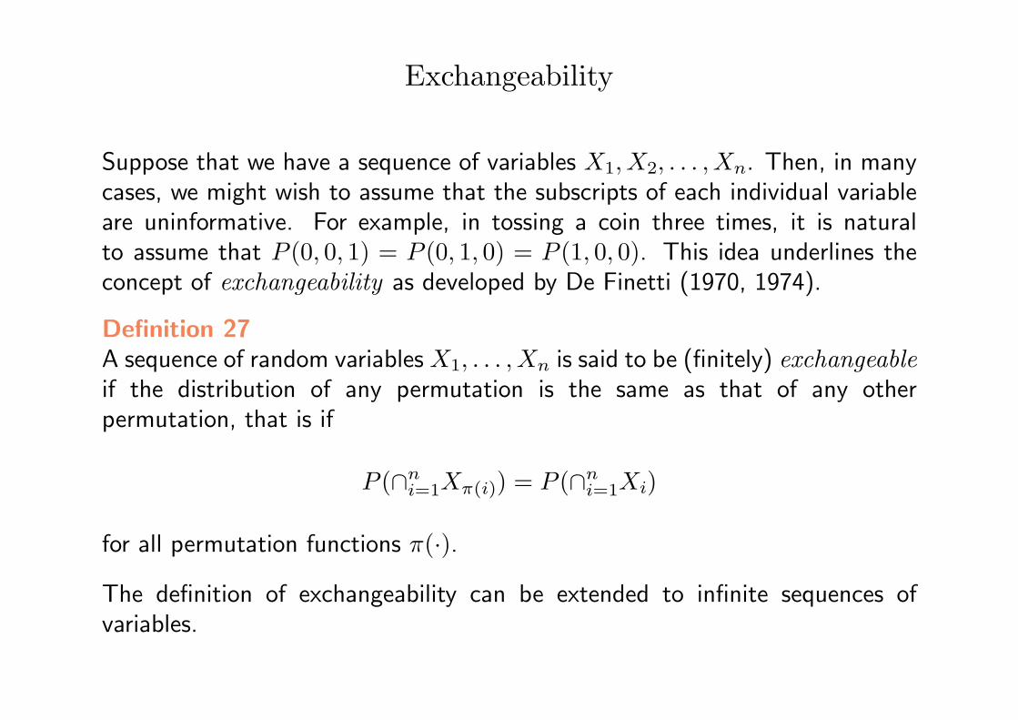
Suppose that we have a sequence of variables X1, X2, . . . , Xn. Then, in manycases, we might wish to assume that the subscripts of each individual variableare uninformative. For example, in tossing a coin three times, it is naturalto assume that P (0, 0, 1) = P (0, 1, 0) = P (1, 0, 0). This idea underlines theconcept of exchangeability as developed by De Finetti (1970, 1974).

Definition 27A sequence of random variablesX1, . . . , Xn is said to be (finitely) exchangeableif the distribution of any permutation is the same as that of any otherpermutation, that is if

P (∩ni=1Xπ(i)) = P (∩ni=1Xi)

for all permutation functions π(·).

The definition of exchangeability can be extended to infinite sequences ofvariables.

Bayesian Statistics

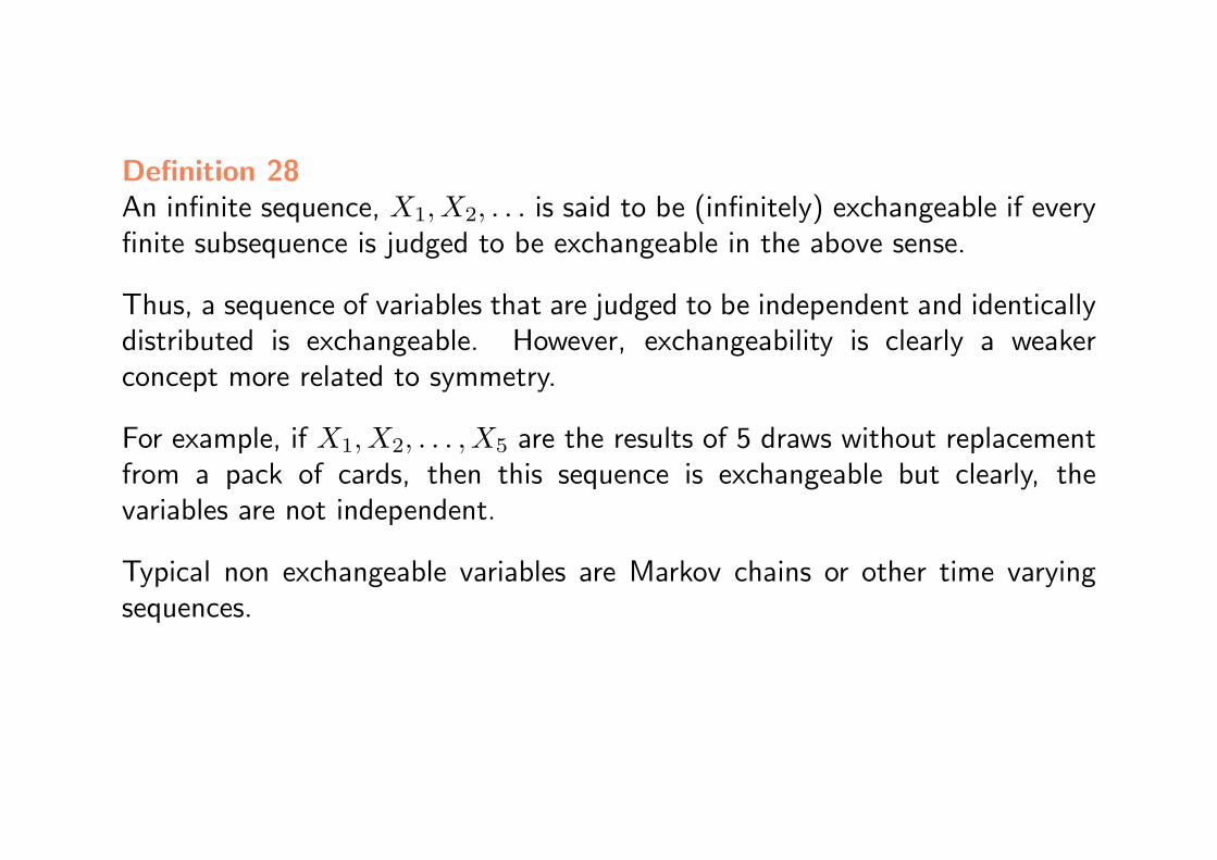
Definition 28An infinite sequence, X1, X2, . . . is said to be (infinitely) exchangeable if everyfinite subsequence is judged to be exchangeable in the above sense.

Thus, a sequence of variables that are judged to be independent and identicallydistributed is exchangeable. However, exchangeability is clearly a weakerconcept more related to symmetry.

For example, if X1, X2, . . . , X5 are the results of 5 draws without replacementfrom a pack of cards, then this sequence is exchangeable but clearly, thevariables are not independent.

Typical non exchangeable variables are Markov chains or other time varyingsequences.

Bayesian Statistics

De Finetti’s theorem for 0-1 random variables

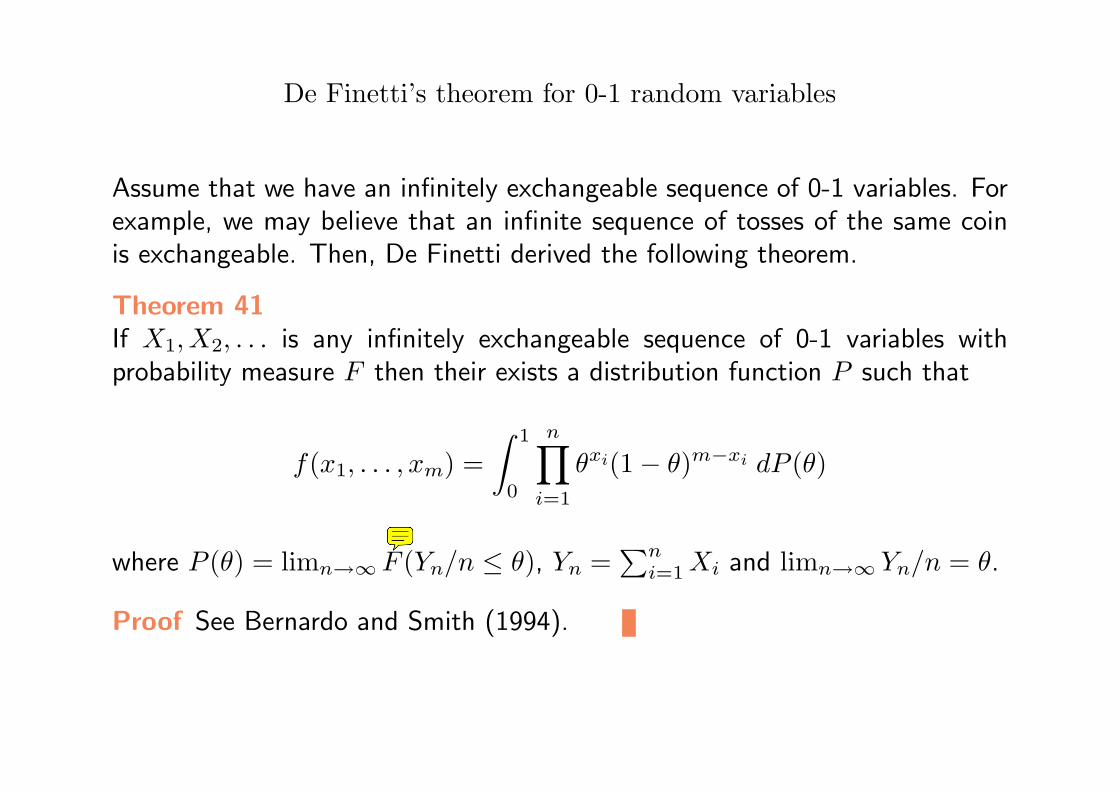
Assume that we have an infinitely exchangeable sequence of 0-1 variables. Forexample, we may believe that an infinite sequence of tosses of the same coinis exchangeable. Then, De Finetti derived the following theorem.

Theorem 41If X1, X2, . . . is any infinitely exchangeable sequence of 0-1 variables withprobability measure F then their exists a distribution function P such that

f(x1, . . . , xm) =∫ 1

0

n∏i=1

θxi(1− θ)m−xi dP (θ)

where P (θ) = limn→∞F (Yn/n ≤ θ), Yn =∑ni=1Xi and limn→∞ Yn/n = θ.

Proof See Bernardo and Smith (1994).

Bayesian Statistics

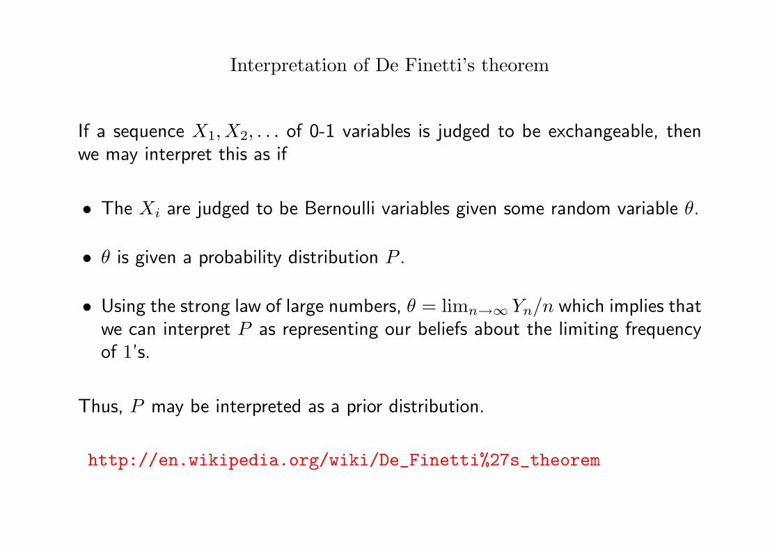
Interpretation of De Finetti’s theorem

If a sequence X1, X2, . . . of 0-1 variables is judged to be exchangeable, thenwe may interpret this as if

• The Xi are judged to be Bernoulli variables given some random variable θ.

• θ is given a probability distribution P .

• Using the strong law of large numbers, θ = limn→∞ Yn/n which implies thatwe can interpret P as representing our beliefs about the limiting frequencyof 1’s.

Thus, P may be interpreted as a prior distribution.

http://en.wikipedia.org/wiki/De_Finetti%27s_theorem

Bayesian Statistics

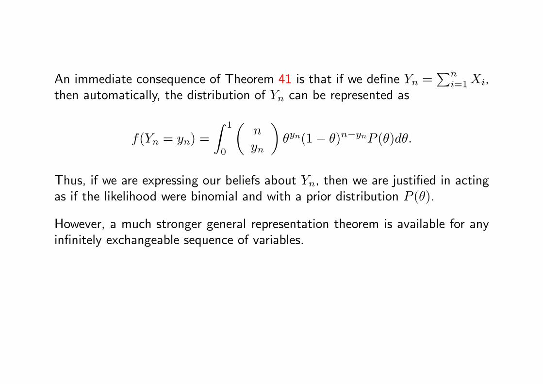
An immediate consequence of Theorem 41 is that if we define Yn =∑ni=1Xi,

then automatically, the distribution of Yn can be represented as

f(Yn = yn) =∫ 1

0

(nyn

)θyn(1− θ)n−ynP (θ)dθ.

Thus, if we are expressing our beliefs about Yn, then we are justified in actingas if the likelihood were binomial and with a prior distribution P (θ).

However, a much stronger general representation theorem is available for anyinfinitely exchangeable sequence of variables.

Bayesian Statistics

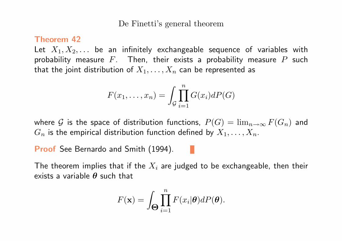
De Finetti’s general theorem

Theorem 42Let X1, X2, . . . be an infinitely exchangeable sequence of variables withprobability measure F . Then, their exists a probability measure P suchthat the joint distribution of X1, . . . , Xn can be represented as

F (x1, . . . , xn) =∫G

n∏i=1

G(xi)dP (G)

where G is the space of distribution functions, P (G) = limn→∞F (Gn) andGn is the empirical distribution function defined by X1, . . . , Xn.

Proof See Bernardo and Smith (1994).

The theorem implies that if the Xi are judged to be exchangeable, then theirexists a variable θ such that

F (x) =∫Θ

n∏i=1

F (xi|θ)dP (θ).

Bayesian Statistics

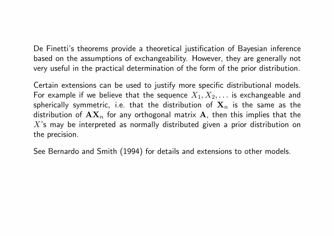
De Finetti’s theorems provide a theoretical justification of Bayesian inferencebased on the assumptions of exchangeability. However, they are generally notvery useful in the practical determination of the form of the prior distribution.

Certain extensions can be used to justify more specific distributional models.For example if we believe that the sequence X1, X2, . . . is exchangeable andspherically symmetric, i.e. that the distribution of Xn is the same as thedistribution of AXn for any orthogonal matrix A, then this implies that theX’s may be interpreted as normally distributed given a prior distribution onthe precision.

See Bernardo and Smith (1994) for details and extensions to other models.

Bayesian Statistics

Hierarchical models

In many models we are unclear about the extent of our prior knowledge.Suppose we have data x with density f(x|θ) where θ = (θ1, . . . , θk). Oftenwe may make extra assumptions about the structural relationships between theelements of θ.

Combining such structural relationships with the assumption of exchangeabilityleads to the construction of prior density, p(θ|φ), for θ which depends upon afurther, unknown hyperparameter φ.

In such cases, following Good (1980), we say that we have a hierarchical model.

Bayesian Statistics

Examples of hierarchical models

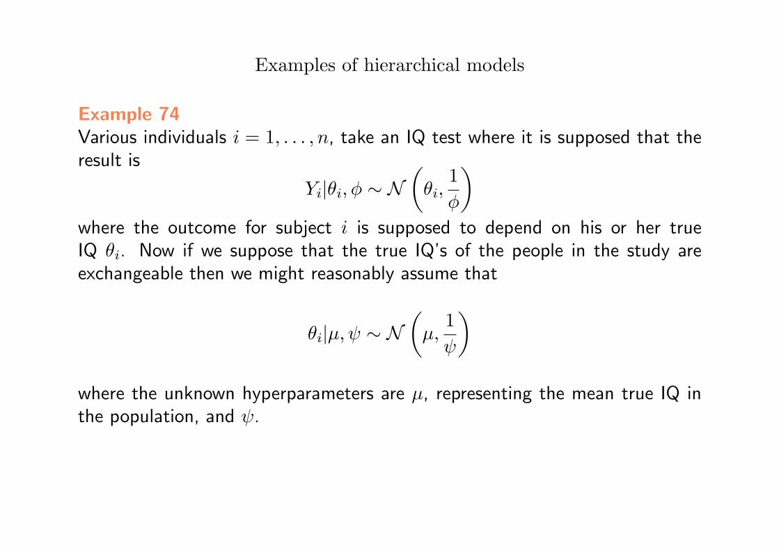
Example 74Various individuals i = 1, . . . , n, take an IQ test where it is supposed that theresult is

Yi|θi, φ ∼ N(θi,

1φ

)where the outcome for subject i is supposed to depend on his or her trueIQ θi. Now if we suppose that the true IQ’s of the people in the study areexchangeable then we might reasonably assume that

θi|µ, ψ ∼ N(µ,

1ψ

)where the unknown hyperparameters are µ, representing the mean true IQ inthe population, and ψ.

Bayesian Statistics

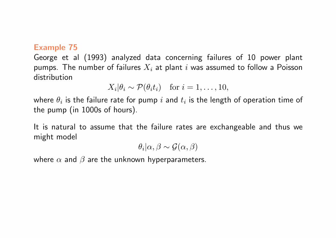
Example 75George et al (1993) analyzed data concerning failures of 10 power plantpumps. The number of failures Xi at plant i was assumed to follow a Poissondistribution

Xi|θi ∼ P(θiti) for i = 1, . . . , 10,

where θi is the failure rate for pump i and ti is the length of operation time ofthe pump (in 1000s of hours).

It is natural to assume that the failure rates are exchangeable and thus wemight model

θi|α, β ∼ G(α, β)

where α and β are the unknown hyperparameters.

Bayesian Statistics

Fitting hierarchical models

The most important problem in dealing with hierarchical models is how to treatthe hyperparameters φ. Usually, there is very little prior information availablewith which to estimate φ.

Thus, two main approaches have developed:

• The natural Bayesian approach is to use relatively uninformative priordistributions for the hyperparameters φ and then perform a fully Bayesiananalysis.

• An alternative is to estimate the hyperparameters using classical statisticalmethods.

This second method is the so-called empirical Bayes approach which we shallexplore below.

Bayesian Statistics

The empirical Bayesian approach

Robbins

This approach is originally due to Robbins (1955). For a full review see

http://en.wikipedia.org/wiki/Empirical_Bayes_method

Bayesian Statistics

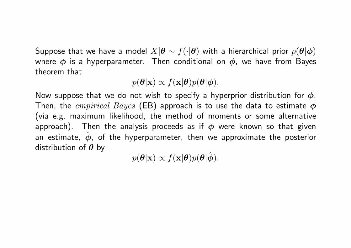
Suppose that we have a model X|θ ∼ f(·|θ) with a hierarchical prior p(θ|φ)where φ is a hyperparameter. Then conditional on φ, we have from Bayestheorem that

p(θ|x) ∝ f(x|θ)p(θ|φ).

Now suppose that we do not wish to specify a hyperprior distribution for φ.Then, the empirical Bayes (EB) approach is to use the data to estimate φ(via e.g. maximum likelihood, the method of moments or some alternativeapproach). Then the analysis proceeds as if φ were known so that givenan estimate, φ, of the hyperparameter, then we approximate the posteriordistribution of θ by

p(θ|x) ∝ f(x|θ)p(θ|φ).

Bayesian Statistics

Multivariate normal example

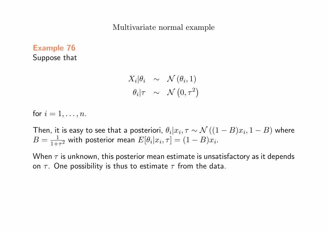
Example 76Suppose that

Xi|θi ∼ N (θi, 1)

θi|τ ∼ N(0, τ2

)for i = 1, . . . , n.

Then, it is easy to see that a posteriori, θi|xi, τ ∼ N ((1−B)xi, 1−B) whereB = 1

1+τ2 with posterior mean E[θi|xi, τ ] = (1−B)xi.

When τ is unknown, this posterior mean estimate is unsatisfactory as it dependson τ . One possibility is thus to estimate τ from the data.

Bayesian Statistics

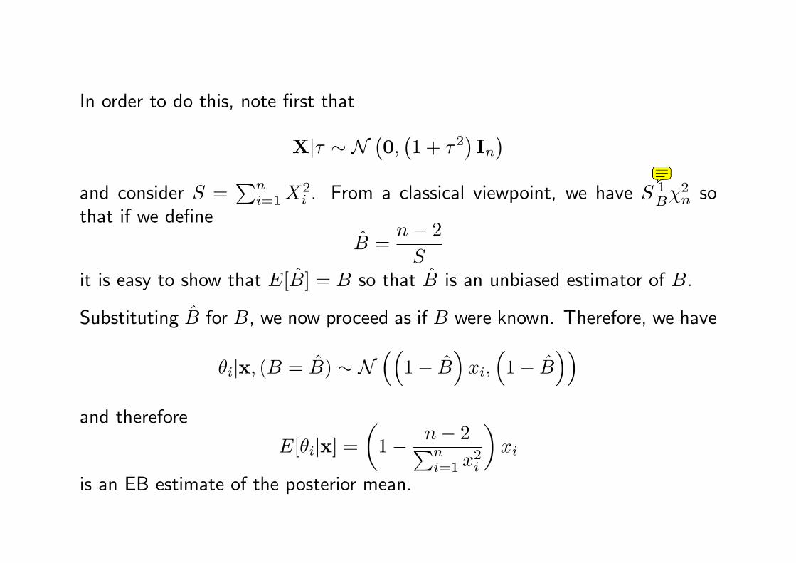
In order to do this, note first that

X|τ ∼ N(0,(1 + τ2

)In)

and consider S =∑ni=1X

2i . From a classical viewpoint, we have S 1

Bχ2n so

that if we define

B =n− 2S

it is easy to show that E[B] = B so that B is an unbiased estimator of B.

Substituting B for B, we now proceed as if B were known. Therefore, we have

θi|x, (B = B) ∼ N((

1− B)xi,(1− B

))and therefore

E[θi|x] =(

1− n− 2∑ni=1 x

2i

)xi

is an EB estimate of the posterior mean.

Bayesian Statistics

Criticisms and characteristics of the empirical Bayes approach

In general, the EB approach leads to compromise (shrinkage) posteriorestimators between the individual (Xi) and group (X) estimators.

One problem with the EB approach is that it clearly ignores the uncertaintyin φ. Another problem with this approach is how to choose the estimatorsof the hyperparameters. Many options are possible, e.g. maximum likelihood,method of moments, unbiased estimators etc. and all will lead to slightlydifferent solutions in general.

This is in contrast to the fully Bayesian approach which requires the definitionof a hyperprior but avoids the necessity of selecting a given value of thehyperprior.

Bayesian Statistics

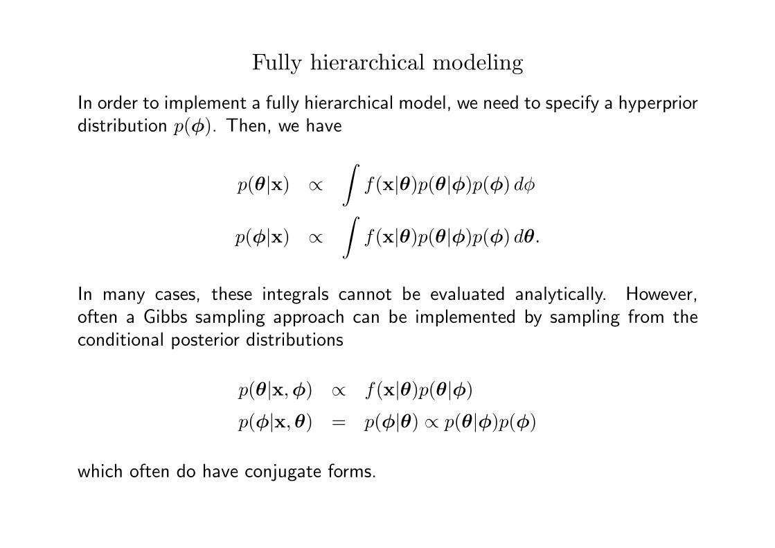
Fully hierarchical modeling

In order to implement a fully hierarchical model, we need to specify a hyperpriordistribution p(φ). Then, we have

p(θ|x) ∝∫f(x|θ)p(θ|φ)p(φ) dφ

p(φ|x) ∝∫f(x|θ)p(θ|φ)p(φ) dθ.

In many cases, these integrals cannot be evaluated analytically. However,often a Gibbs sampling approach can be implemented by sampling from theconditional posterior distributions

p(θ|x,φ) ∝ f(x|θ)p(θ|φ)

p(φ|x,θ) = p(φ|θ) ∝ p(θ|φ)p(φ)

which often do have conjugate forms.

Bayesian Statistics

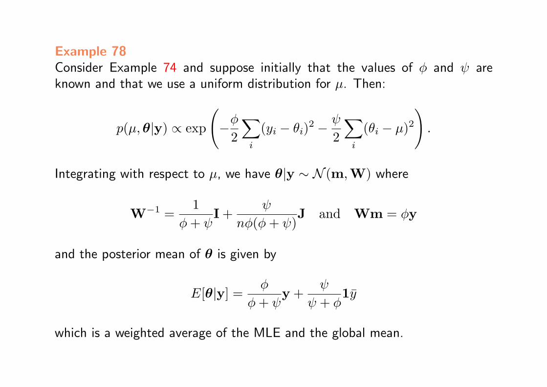
Example 78Consider Example 74 and suppose initially that the values of φ and ψ areknown and that we use a uniform distribution for µ. Then:

p(µ,θ|y) ∝ exp

(−φ

2

∑i

(yi − θi)2 −ψ

2

∑i

(θi − µ)2).

Integrating with respect to µ, we have θ|y ∼ N (m,W) where

W−1 =1

φ+ ψI +

ψ

nφ(φ+ ψ)J and Wm = φy

and the posterior mean of θ is given by

E[θ|y] =φ

φ+ ψy +

ψ

ψ + φ1y

which is a weighted average of the MLE and the global mean.

Bayesian Statistics

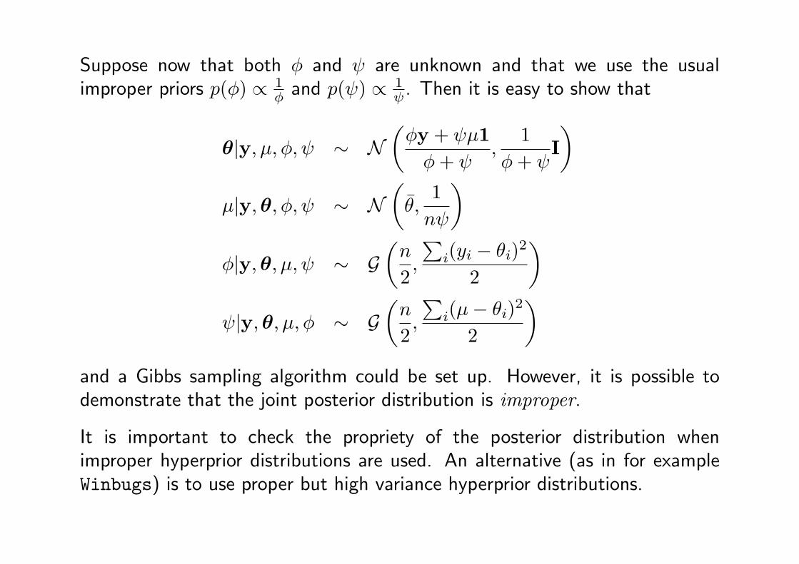
Suppose now that both φ and ψ are unknown and that we use the usualimproper priors p(φ) ∝ 1

φ and p(ψ) ∝ 1ψ. Then it is easy to show that

θ|y, µ, φ, ψ ∼ N(φy + ψµ1φ+ ψ

,1

φ+ ψI)

µ|y,θ, φ, ψ ∼ N(θ,

1nψ

)φ|y,θ, µ, ψ ∼ G

(n

2,

∑i(yi − θi)2

2

)ψ|y,θ, µ, φ ∼ G

(n

2,

∑i(µ− θi)2

2

)and a Gibbs sampling algorithm could be set up. However, it is possible todemonstrate that the joint posterior distribution is improper.

It is important to check the propriety of the posterior distribution whenimproper hyperprior distributions are used. An alternative (as in for exampleWinbugs) is to use proper but high variance hyperprior distributions.

Bayesian Statistics

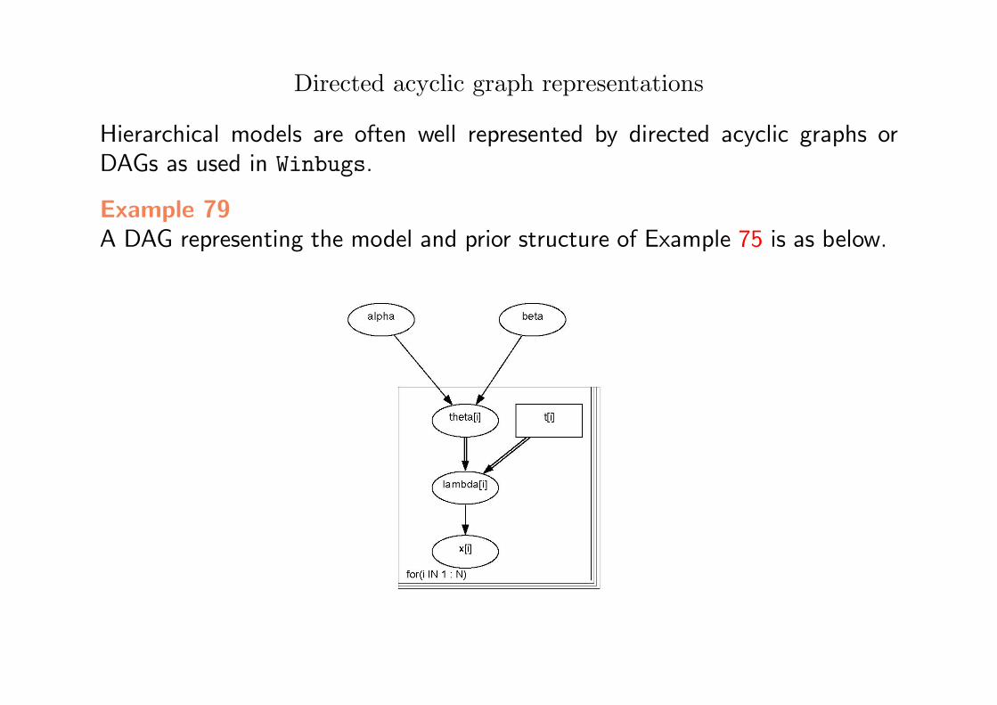
Directed acyclic graph representations

Hierarchical models are often well represented by directed acyclic graphs orDAGs as used in Winbugs.

Example 79A DAG representing the model and prior structure of Example 75 is as below.

Bayesian Statistics

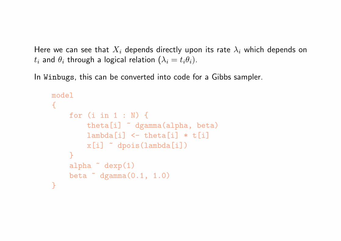
Here we can see that Xi depends directly upon its rate λi which depends onti and θi through a logical relation (λi = tiθi).

In Winbugs, this can be converted into code for a Gibbs sampler.

model{

for (i in 1 : N) {theta[i] ~ dgamma(alpha, beta)lambda[i] <- theta[i] * t[i]x[i] ~ dpois(lambda[i])

}alpha ~ dexp(1)beta ~ dgamma(0.1, 1.0)

}

Bayesian Statistics

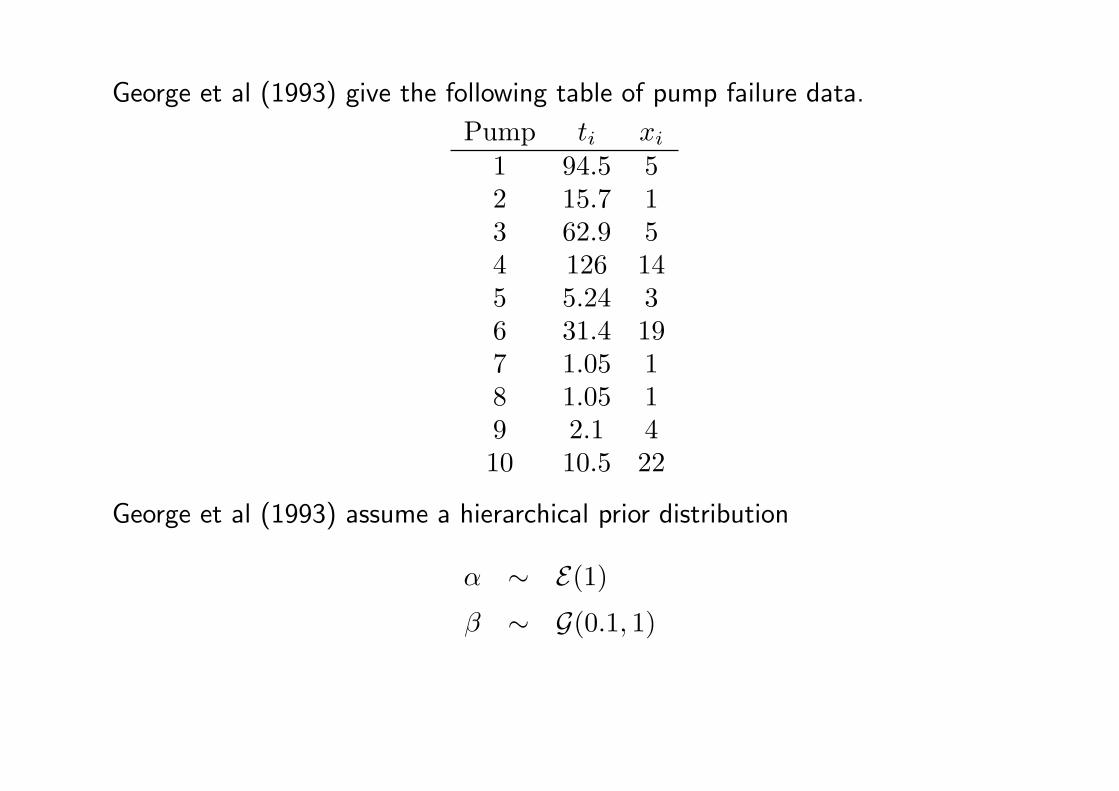
George et al (1993) give the following table of pump failure data.

Pump ti xi1 94.5 52 15.7 13 62.9 54 126 145 5.24 36 31.4 197 1.05 18 1.05 19 2.1 410 10.5 22

George et al (1993) assume a hierarchical prior distribution

α ∼ E(1)

β ∼ G(0.1, 1)

Bayesian Statistics

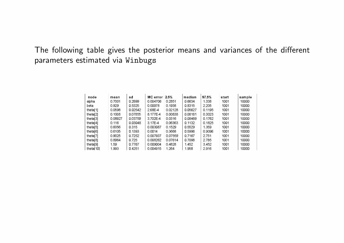
The following table gives the posterior means and variances of the differentparameters estimated via Winbugs

Bayesian Statistics

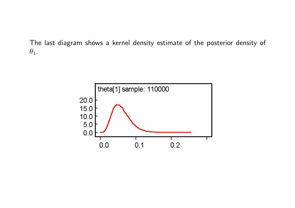
The last diagram shows a kernel density estimate of the posterior density ofθ1.

Bayesian Statistics