10. Graph Matrices

Since a graph is completely determined by specifying either its adjacency structure or itsincidence structure, these specifications provide far more efficient ways of representing alarge or complicated graph than a pictorial representation. As computers are more adept atmanipulating numbers than at recognising pictures, it is standard practice to communicatethe specification of a graph to a computer in matrix form. In this chapter, we study varioustypes of matrices associated with a graph, and our study is based on Narsing Deo [63],Foulds [82], Harary [104] and Parthasarathy [180].

10.1 Incidence Matrix

Let G be a graph with n vertices, m edges and without self-loops. The incidence matrix A ofG is an n×m matrix A = [ai j] whose n rows correspond to the n vertices and the m columnscorrespond to m edges such that

ai j =

{

1 , i f jth edge m j is incident on the ith vertex

0 , otherwise.

It is also called vertex-edge incidence matrix and is denoted by A(G).Example Consider the graphs given in Figure 10.1. The incidence matrix of G1 is

e1 e2 e3 e4 e5 e6 e7 e8

A(G1) =

v1

v2

v3

v4

v5

v6

0 0 0 1 0 1 0 0

0 0 0 0 1 1 1 1

0 0 0 0 0 0 0 1

1 1 1 0 1 0 0 0

0 0 1 1 0 0 1 0

1 1 0 0 0 0 0 0

.

The incidence matrix of G2 is

264 Graph Matrices

e1 e2 e3 e4 e5

A(G2) =

v1

v2

v3

v4

1 1 0 0 0

1 0 0 1 1

0 1 1 1 1

0 0 1 0 0

.

The incidence matrix of G3 is

e1 e2 e3 e4 e5

A(G3) =

v1

v2

v3

v4

1 1 0 0 1

1 1 1 0 0

0 0 0 1 0

0 0 1 1 1

.

Fig. 10.1

The incidence matrix contains only two types of elements, 0 and 1. This clearly is abinary matrix or a (0, 1)-matrix.

We have the following observations about the incidence matrix A.

1. Since every edge is incident on exactly two vertices, each column of A has exactlytwo one’s.

2. The number of one’s in each row equals the degree of the corresponding vertex.

Graph Theory 265

3. A row with all zeros represents an isolated vertex.

4. Parallel edges in a graph produce identical columns in its incidence matrix.

5. If a graph is disconnected and consists of two components G1 and G2, the incidencematrix A(G) of graph G can be written in a block diagonal form as

A(G) =

[

A(G1) 0

0 A(G2)

]

,

where A(G1) and A(G2) are the incidence matrices of components G1 and G2. Thisobservation results from the fact that no edge in G1 is incident on vertices of G2 andvice versa. Obviously, this is also true for a disconnected graph with any number ofcomponents.

6. Permutation of any two rows or columns in an incidence matrix simply correspondsto relabeling the vertices and edges of the same graph.

Note The matrix A has been defined over a field, Galois field modulo 2 or GF(2), thatis, the set {0,1} with operation addition modulo 2 written as + such that 0 +0 = 0, 1 +0 =1, 1+1 = 0 and multiplication modulo 2 written as“.” such that 0.0 = 0, 1.0 = 0 = 0.1, 1.1 = 1.

The following result is an immediate consequence of the above observations.

Theorem 10.1 Two graphs G1 and G2 are isomorphic if and only if their incidence ma-trices A(G1) and A(G2) differ only by permutation of rows and columns.

Proof Let the graphs G1 and G2 be isomorphic. Then there is a one-one correspondencebetween the vertices and edges in G1 and G2 such that the incidence relation is preserved.Thus A(G1) and A(G2) are either same or differ only by permutation of rows and columns.

The converse follows, since permutation of any two rows or columns in an incidencematrix simply corresponds to relabeling the vertices and edges of the same graph. q

Rank of the incidence matrix

Let G be a graph and let A(G) be its incidence matrix. Now each row in A(G) is a vectorover GF(2) in the vector space of graph G. Let the row vectors be denoted by A1, A2, . . .,An. Then,

A(G) =

A1

A2

.

.

.An

.

266 Graph Matrices

Since there are exactly two ones in every column of A, the sum of all these vectors is 0

(this being a modulo 2 sum of the corresponding entries).Thus vectors A1, A2, . . . , An are linearly dependent. Therefore, rank A < n.

Hence, rank A ≤ n−1.

From the above observations, we have the following result.

Theorem 10.2 If A(G) is an incidence matrix of a connected graph G with n vertices,then rank of A(G) is n−1.

Proof Let G be a connected graph with n vertices and let the number of edges in G be m.Let A(G) be the incidence matrix and let A1, A2, . . ., An be the row vector of A(G).

Then, A(G) =

A1

A2

.

.

.An

. (10.2.1)

Clearly, rank A(G) ≤ n−1. (10.2.2)

Consider the sum of any m of these row vectors, m ≤ n−1. Since G is connected, A(G)cannot be partitioned in the form

A(G) =

[

A(G1) 0

0 A(G2)

]

such that A(G1) has m rows and A(G2) has n−m rows.Thus there exists no m×m submatrix of A(G) for m ≤ n−1, such that the modulo 2 sum

of these m rows is equal to zero.As there are only two elements 0 and 1 in this field, the additions of all vectors taken m

at a time for m = 1, 2, . . ., n−1 gives all possible linear combinations of n−1 row vectors.Thus no linear combinations of m row vectors of A, for m ≤ n−1, is zero.

Therefore, rank A(G) ≤ n−1. (10.2.3)

Combining (10.2.2) and (10.2.3), it follows that rank A(G) = n−1. q

Remark If G is a disconnected graph with k components, then it follows from the abovetheorem that rank of A(G) is n− k.

Let G be a connected graph with n vertices and m edges. Then the order of the incidencematrix A(G) is n×m. Now, if we remove any one row from A(G), the remaining (n−1) bym submatrix is of rank (n−1). Thus the remaining (n−1) row vectors are linearly indepen-dent. This shows that only (n−1) rows of an incidence matrix are required to specify the

Graph Theory 267

corresponding graph completely, because (n−1) rows contain the same information as theentire matrix. This follows from the fact that given (n−1) rows, we can construct the nthrow, as each column in the matrix has exactly two ones. Such an (n−1) × m matrix of A

is called a reduced incidence matrix and is denoted by A f . The vertex corresponding to thedeleted row in A f is called the reference vertex. Obviously, any vertex of a connected graphcan be treated as the reference vertex.

The following result gives the nature of the incidence matrix of a tree.

Theorem 10.3 The reduced incidence matrix of a tree is non-singular.

Proof A tree with n vertices has n−1 edges and also a tree is connected. Therefore, thereduced incidence matrix is a square matrix of order n−1, with rank n−1. Thus the resultfollows.

Now a graph G with n vertices and n − 1 edges which is not a tree is obviously dis-connected. Therefore the rank of the incidence matrix of G is less than (n−1). Hence the(n−1)×(n−1) reduced incidence matrix of a graph is non-singular if and only if the graphis a tree. q

10.2 Submatrices of A(G)

Let H be a subgraph of a graph G, and let A(H) and A(G) be the incidence matrices of H

and G respectively. Clearly, A(H) is a submatrix of A(G), possibly with rows or columnspermuted. We observe that there is a one-one correspondence between each n×k submatrixof A(G) and a subgraph of G with k edges, k being a positive integer, k < m and n being thenumber of vertices in G.

The following is a property of the submatrices of A(G).

Theorem 10.4 Let A(G) be the incidence matrix of a connected graph G with n ver-tices. An (n− 1)× (n− 1) submatrix of A(G) is non-singular if and only if the n− 1 edgescorresponding to the n−1 columns of this matrix constitutes a spanning tree in G.

Proof Let G be a connected graph with n vertices and m edges. So, m ≥ n−1.Let A(G) be the incidence matrix of G, so that A(G) has n rows and m columns (m≥ n−1).We know every square submatrix of order (n− 1)× (n− 1) in A(G) is the reduced inci-

dence matrix of some subgraph H in G with n−1 edges, and vice versa. We also know thata square submatrix of A(G) is non-singular if and only if the corresponding subgraph is atree.

Obviously, the tree is a spanning tree because it contains n − 1 edges of the n-vertexgraph.

Hence (n − 1)× (n − 1) submatrix of A(G) is non-singular if and only if n − 1 edgescorresponding to n−1 columns of this matrix forms a spanning tree. q

268 Graph Matrices

The following is another form of incidence matrix.

Definition: The matrix F = [ fi j] of the graph G = (V, E) with V = {v1, v2, . . . , vn} andE = {e1, e2, . . ., em}, is the n×m matrix associated with a chosen orientation of the edgesof G in which for each e = (vi, v j), one of vi or v j is taken as positive end and the other asnegative end, and is defined by

fi j =

1 , i f vi is the positive end o f e j ,−1 , i f vi is the negative end o f e j ,0 , i f vi is not incident with e j .

This matrix F can also be obtained from the incidence matrix A by changing either ofthe two 1s to −1 in each column.

The above arguments amount to arbitrarily orienting the edges of G, and F is then theincidence matrix of the oriented graph.

The matrix F is then the modified definition of the incidence matrix A.

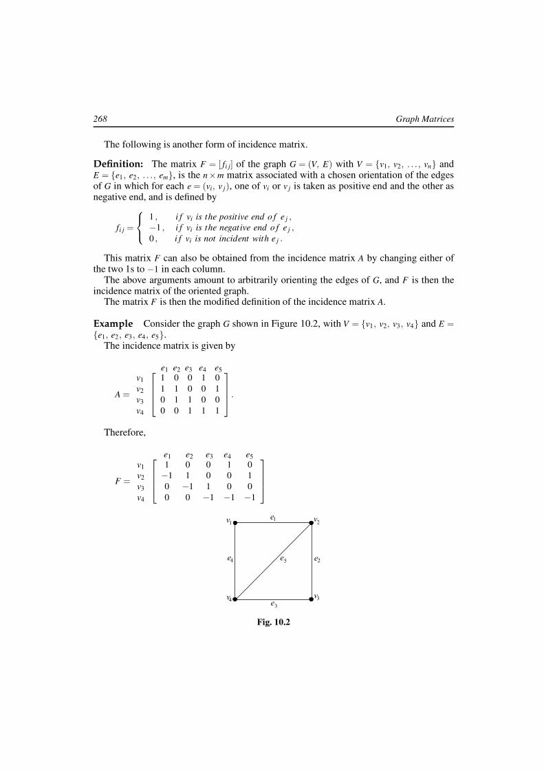
Example Consider the graph G shown in Figure 10.2, with V = {v1, v2, v3, v4} and E ={e1, e2, e3, e4, e5}.

The incidence matrix is given by

e1 e2 e3 e4 e5

A =

v1

v2

v3

v4

1 0 0 1 0

1 1 0 0 1

0 1 1 0 0

0 0 1 1 1

.

Therefore,

e1 e2 e3 e4 e5

F =

v1

v2

v3

v4

1 0 0 1 0

−1 1 0 0 1

0 −1 1 0 0

0 0 −1 −1 −1

Fig. 10.2

Graph Theory 269

Theorem 10.5 If G is a connected graph with n vertices, then rank F = n−1.

Proof Let G be a connected graph with V = {v1, v2, . . ., vn} and E = {e1, e2, . . ., em}.Then the matrix F = [ fi j]n×m is given by

fi j =

1 , i f vi is the positive end o f e j ,−1 , i f vi is the negative end o f e j ,0 , i f vi is not incident with e j .

Let R j be the jth row of F . Since each column of F has only one +1 and one −1, asnon-zero entries, rank F < n. Thus, rank F ≤ n−1.

Now, letn

∑1

c jR j = 0 be any other linear dependence relation of R1, R2, . . ., Rn with at least

one c j non-zero.If cr 6= 0, then the row Rr has non-zero entries in those columns which correspond to

edges incident with vr . For each such column there is just one row, say Rs, at which there isa non-zero entry (with opposite sign to the non-zero entry in Rr). The dependence relationthus requires cs = cr, for all s corresponding to vertices adjacent to vr. Since G is connected,

we have c j = c, for all j = 1, 2, . . ., n. Therefore the dependence relation is c

(

n

∑1

R j

)

= 0,

which is same as the first one. Hence, rank F = n−1.

Alternative Proof

Then

F =

R1

R2

M

Rn

. (10.5.1)

Since each column of F has only one +1 and one −1 as non-zero entries,n

∑j=1

R j = 0.

Thus, rank F ≤ n−1. (10.5.2)

Consider the sum of any m of these row vectors, m ≤ n−1. As G is connected, F cannot

be partitioned in the form F =

[

F1 0

0 F2

]

, such that F1 has m rows and F2 as n−m rows.

Therefore there exists no m×m submatrix of F for m ≤ n−1, such that the sum of these m

rows is equal to zero. Therefore,

m

∑j=1

R j 6= 0. (10.5.3)

270 Graph Matrices

Also, there is no linear combination of m(m ≤ n−1) vectors of F, which is zero. For, ifm

∑j=1

c jR j = 0 is a linear combination, with at least one c j non-zero, say cr 6= 0, then the row

Rr has non-zero entries in those columns which correspond to edges incident with vr . Sofor each such column there is just one row, say Rs at which there is a non-zero entry withopposite sign to the non-zero entry in Rr. The linear combination thus requires cs = cr forall s corresponding to vertices adjacent to vr. As G is connected, we have c j = c, for all

j = 1, . . .,m. Therefore the linear combination becomes c(m

∑j=1

R j ) = 0, orm

∑j=1

R j = 0, which

contradicts (10.5.3).

Hence, rank F = n−1. q

Theorem 10.6 If G is a disconnected graph with k components, then rank F = n− k.

Proof Since G has k components, F can be partitioned as

F =

F1 0 0 · · · 0

0 F2 0 · · · 0

0 0 F3 · · · 0

...0 0 0 · · · Fk

,

where Fi is the matrix of the ith component Gi of G. We have proved that rank Fi = ni −1,where ni is the number of vertices in Gi.

Thus, rank F = n1 −1 +n2−1 + . . .+nk −1 = n1 +n2 + . . .+nk − k = n− k,

as the number of vertices in G is n1 +n2 + . . .+nk = n. q

Corollary 10.1 A basis for the row space of F is obtained by taking for each i, 1 ≤ i ≤ k,any ni −1 rows of Fi.

Theorem 10.7 The determinant of any square submatrix of the matrix F of a graph G

has value 1, −1, or zero.

Proof Let N be the square submatrix of F such that N has both non-zero entries +1 and−1 in each column. Then row sum of N is zero and hence |N| = 0. Clearly if N has nonon-zero entries, then |N|= 0.

Now let some column of N have only one non-zero entry. Then expanding |N| with thehelp of this column, we get |N| = ±|N ′|, where N ′ is a matrix obtained by omitting a rowand column of N. Continuing in this way, we either get a matrix whose determinant is zero,or end up with a single non-zero entry of N, in which case |N|= ±1. q

Graph Theory 271

Theorem 10.8 Let X be any set of n− 1 edges of the connected graph G = (V, E) andFx the (n− 1)× (n− 1) submatrix of the matrix F of G, determined by any n− 1 rows andthose columns which correspond to the edges of X . Then Fx is non-singular if and only ifthe edge induced subgraph < X > of G is a spanning tree of G.

Proof Let F ′ be the matrix corresponding to < X >. If < X > is a spanning tree of G, thenFx consists of n−1 rows of F ′. Since < X > is connected, therefore rank Fx = n−1. HenceFx is non-singular.

Conversely, let Fx be non-singular. Then F ′ contains an (n− 1)× (n− 1) non singularsubmatrix. Therefore, rank F ′ = n− 1. Since rank + nullity = m, for any graph G, andm(< X >) = n−1 and rank (< X >) = n−1, therefore, nullity (< X >) = 0. Thus < X > isacyclic and connected and so is a spanning tree of G. q

10.3 Cycle Matrix

Let the graph G have m edges and let q be the number of different cycles in G. The cyclematrix B = [bi j]q×m of G is a (0, 1)− matrix of order q×m, with bi j = 1, if the ith cycleincludes jth edge and bi j = 0, otherwise. The cycle matrix B of a graph G is denoted byB(G).

Example Consider the graph G1 given in Figure 10.3.

Fig. 10.3

The graph G1 has four different cycles Z1 = {e1, e2}, Z2 = {e3, e5, e7}, Z3 = {e4, e6, e7}and Z4 = {e3, e4, e6, e5}.

The cycle matrix is

272 Graph Matrices

e1 e2 e3 e4 e5 e6 e7 e8

B(G1) =

z1

z2

z3

z4

1 1 0 0 0 0 0 0

0 0 1 0 1 0 1 0

0 0 0 1 0 1 1 0

0 0 1 1 1 1 0 0

.

The graph G2 of Figure 10.3 has seven different cycles, namely, Z1 = {e1, e2},Z2 = {e2, e7, e8}, Z3 = {e1, e7, e8}, Z4 = {e4, e5, e6, e7}, Z5 = {e2, e4, e5, e6, e8},Z6 = {e1, e4, e5, e6, e8} and Z7 = {e9}. The cycle matrix is given by

e1 e2 e3 e4 e5 e6 e7 e8 e9

B(G2) =

z1

z2

z3

z4

z5

z6

z7

1 1 0 0 0 0 0 0 0

0 1 0 0 0 0 1 1 0

1 0 0 0 0 0 1 1 0

0 0 0 1 1 1 1 0 0

0 1 0 1 1 1 0 1 0

1 0 0 1 1 1 0 1 0

0 0 0 0 0 0 0 0 1

.

We have the following observations regarding the cycle matrix B(G) of a graph G.

1. A column of all zeros corresponds to a non cycle edge, that is, an edge which doesnot belong to any cycle.

2. Each row of B(G) is a cycle vector.

3. A cycle matrix has the property of representing a self-loop and the correspondingrow has a single one.

4. The number of ones in a row is equal to the number of edges in the correspondingcycle.

5. If the graph G is separable (or disconnected) and consists of two blocks (or compo-nents) H1 and H2, then the cycle matrix B(G) can be written in a block-diagonal formas

B(G) =

[

B(H1) 0

0 B(H2)

]

,

where B(H1) and B(H2) are the cycle matrices of H1 and H2. This follows from thefact that cycles in H1 have no edges belonging to H2 and vice versa.

6. Permutation of any two rows or columns in a cycle matrix corresponds to relabelingthe cycles and the edges.

Graph Theory 273

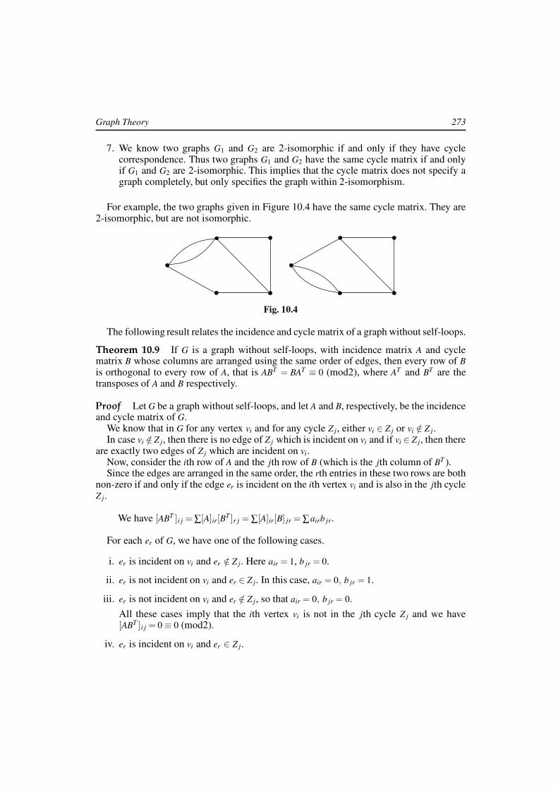
7. We know two graphs G1 and G2 are 2-isomorphic if and only if they have cyclecorrespondence. Thus two graphs G1 and G2 have the same cycle matrix if and onlyif G1 and G2 are 2-isomorphic. This implies that the cycle matrix does not specify agraph completely, but only specifies the graph within 2-isomorphism.

For example, the two graphs given in Figure 10.4 have the same cycle matrix. They are2-isomorphic, but are not isomorphic.

Fig. 10.4

The following result relates the incidence and cycle matrix of a graph without self-loops.

Theorem 10.9 If G is a graph without self-loops, with incidence matrix A and cyclematrix B whose columns are arranged using the same order of edges, then every row of B

is orthogonal to every row of A, that is ABT = BAT ≡ 0 (mod2), where AT and BT are thetransposes of A and B respectively.

Proof Let G be a graph without self-loops, and let A and B, respectively, be the incidenceand cycle matrix of G.

We know that in G for any vertex vi and for any cycle Z j, either vi ∈ Z j or vi /∈ Z j.In case vi /∈ Z j, then there is no edge of Z j which is incident on vi and if vi ∈ Z j, then there

are exactly two edges of Z j which are incident on vi.Now, consider the ith row of A and the jth row of B (which is the jth column of BT ).Since the edges are arranged in the same order, the rth entries in these two rows are both

non-zero if and only if the edge er is incident on the ith vertex vi and is also in the jth cycleZ j.

We have [ABT ]i j = ∑[A]ir[BT ]r j = ∑[A]ir[B] jr = ∑airb jr.

For each er of G, we have one of the following cases.

i. er is incident on vi and er /∈ Z j. Here air = 1, b jr = 0.

ii. er is not incident on vi and er ∈ Z j. In this case, air = 0, b jr = 1.

iii. er is not incident on vi and er /∈ Z j, so that air = 0, b jr = 0.

All these cases imply that the ith vertex vi is not in the jth cycle Z j and we have[ABT ]i j = 0 ≡ 0 (mod2).

iv. er is incident on vi and er ∈ Z j.

274 Graph Matrices

Here we have exactly two edges, say er and et incident on vi so that air = 1, ait = 1,b jr = 1, b jt = 1. Therefore, [ABT ]i j = ∑airb jr = 1 +1 ≡ 0 (mod2). q

We illustrate the above theorem with the following example (Fig. 10.5).

Fig. 10.5

Clearly,

ABT =

0 0 0 1 0 1 0 0

0 0 0 0 1 1 1 1

0 0 0 0 0 0 0 1

1 1 1 0 1 0 0 0

0 0 1 1 0 0 1 0

1 1 0 0 0 0 0 0

1 0 0 0

1 0 0 0

0 1 0 1

0 0 1 1

0 1 0 1

0 0 1 1

0 1 1 0

0 0 0 0

=

0 0 2 2

0 2 2 2

0 0 0 0

2 2 0 2

0 2 2 2

2 0 0 0

≡ 0(mod2).

We know that a set of fundamental cycles (or basic cycles) with respect to any spanningtree in a connected graph are the only independent cycles in a graph. The remaining cyclescan be obtained as ring sums (i.e., linear combinations) of these cycles. Thus, in a cyclematrix, if we take only those rows that correspond to a set of fundamental cycles andremove all other rows, we do not lose any information. The removed rows can be formedfrom the rows corresponding to the set of fundamental cycles. For example, in the cyclematrix of the graph given in Figure 10.6, the fourth row is simply the mod 2 sum of thesecond and the third rows. Fundamental cycles are

Graph Theory 275

Z1 = {e1, e2, e4, e7}Z2 = {e3, e4, e7}Z3 = {e5, e6, e7}

Fig. 10.6

e2 e3 e6 e1 e4 e5 e7

Z1

Z2

Z3

1 0 0... 1 1 0 1

0 1 0... 0 1 0 1

0 0 1... 0 0 1 1

.

A submatrix of a cycle matrix in which all rows correspond to a set of fundamentalcycles is called a fundamental cycle matrix B f .

The permutation of rows and/or columns do not affect B f . If n is the number of vertices,m the number of edges in a connected graph G, then B f is an (m−n+1)×m matrix becausethe number of fundamental cycles is m−n +1, each fundamental cycle being produced byone chord.

Now, arranging the columns in B f such that all the m− n + 1 chords correspond to thefirst m−n +1 columns and rearranging the rows such that the first row corresponds to thefundamental cycle made by the chord in the first column, the second row to the fundamentalcycle made by the second, and so on. This arrangement is done for the above fundamentalcycle matrix.

A matrix B f thus arranged has the form

B f = [Iµ : Bt ],

where Iµ is an identity matrix of order µ = m− n + 1 and Bt is the remaining µ × (n− 1)submatrix, corresponding to the branches of the spanning tree.

From equation B f = [Iµ : Bt ], we have rank B f = µ = m−n +1.Since B f is a submatrix of the cycle matrix B, therefore, rank B ≥ rank B f and thus,

rank B ≥ m−n +1.

The following result gives the rank of the cycle matrix.

276 Graph Matrices

Theorem 10.10 If B is a cycle matrix of a connected graph G with n vertices and m

edges, then rank B = m−n +1.

Proof Let A be the incidence matrix of the connected graph G.

Then ABT ≡ 0(mod2).

Using Sylvester’s theorem (Theorem 10.13), we have rank A+ rank BT ≤ m so thatrank A+ rank B ≤ m.

Therefore, rank B ≤ m− rank A.

As rank A = n−1, we get rank B ≤ m− (n−1) = m−n +1.

But, rank B ≥ m−n +1.

Combining, we get rank B = m−n +1. q

Theorem 10.10 can be generalised in the following form.

Theorem 10.11 If B is a cycle matrix of a disconnected graph G with n vertices, m edgesand k components, then rank B = m−n + k.

Proof Let B be the cycle matrix of the disconnected graph G with n vertices, m edgesand k components. Let the k components be G1, G2, ...,Gk with n1,n2, ...,nk vertices and m1,m2, . . .,mk edges respectively.

Then n1 +n2 + . . .+nk = n and m1 +m2 + ...+mk = m.

Let B1, B2, . . ., Bk be the cycle matrices of G1, G2, . . . , Gk.

Then B(G) =

B1(G1) 0 0 · · · 0

0 B2(G2) 0 · · · 0

0 0 B3(G3) · · · 0

...0 0 0 · · · Bk(Gk)

.

We know rank Bi = mi −ni +1, for 1 ≤ i ≤ k.

Therefore, rank B = rank B1 + . . .+ rank Bk

= (m1 −n1 +1)+ . . .+(mk −nk +1)

= (m1 + . . .+mk)− (n1 + . . .+nk)+ k = m−n + k. q

Graph Theory 277

Definition: Let A be a matrix of order k×m, with k < m. The major determinant of A isthe determinant of the largest square submatrix of A, formed by taking any k columns of A.That is, the determinant of any k×k square submatrix is called the major determinant of A.

Let A and B be matrices of orders k ×m and m × k respectively (k < m). If columnsi1, i2, . . ., ik of B are chosen for a particular major of B, then the corresponding major in A

consists of the rows i1, i2, . . ., ik in A.If A is a square matrix of order n, then AX = 0 has a non trivial solution X 6= 0 if and only

if A is singular, that is |A| = 0. The set of all vectors X that satisfy AX = 0 forms a vectorspace called the null space of matrix A. The rank of the null space is called the nullity of A.Further more,

rank A+nullityA = n.

These definitions and the above equation also hold when A is a matrix of order k×n, k < n.

We now give Binet-Cauchy and Sylvester theorems which will be used in the furtherdiscussions.

Theorem 10.12 (Binet−Cauchy) If A and B are two matrices of the order k×m and m×k respectively (k < m), then |AB|= sum of the products of corresponding major determinantsof A and B.

Proof We multiply two (m+ k)× (m+ k) partitioned matrices to get

[

Ik A

O Im

][

A O

−Im B

]

=

[

O AB

−Im B

]

,

where Im and Ik are identity matrices of order m and k respectively.

Therefore, det

[

A O

−Im B

]

= det

[

O AB

−Im B

]

.

Thus, det(AB) =det

[

A O

−Im B

]

. (10.12.1)

Now apply Cauchy’s expansion method to the right side of (10.12.1) and observe that theonly non-zero minors of any order in −Im are its principal minors of that order. Therefore,we see that the Cauchy expansion consists of these minors of order m− k multiplied bytheir cofactors of order k in A and B together. q

Theorem 10.13 (Sylvester) If A and B are matrices of order k×m and n× p respectively,then nullity AB ≤ nullity A+ nullity B.

Proof Since every vector X satisfying BX = 0 also satisfies ABX = 0, therefore we have

nullity AB ≥ nullity B ≥ 0. (10.13.1)

278 Graph Matrices

Let nullity B = s. So there exists a set of s linearly independent vectors {x1, x2, . . ., xs}forming a basis of the null space of B. Therefore,

BXi = 0, for i = 1, 2, . . ., s. (10.13.2)

Now let nullity AB = s + t . Thus there exists a set of t linearly independent vectors[Xs+1, Xs+2, . . . , Xs+t ] such that the set {X1, X2, . . . , Xs, Xs+1, . . ., Xs+t} forms a basis forthe null space of AB. Therefore,

ABXi = 0, for i = 1, 2, . . . , s, s+1, . . . , s+ t . (10.13.3)

This implies that out of the s+ t vectors Xi forming a basis of the null space of AB, thefirst s vectors are made zero by B and the remaining non-zero BXi’s, i = s + 1, . . ., s + t aremade zero by A.

Clearly, the vectors BXs+1, . . ., BXs+t are linearly independent. For if

b1BXs+1 +b2BXs+2 + . . .+btBXs+t = 0,

i.e., if B(b1Xs+1 +b2Xs+2 + . . .+btXs+t) = 0,

then the vector b1Xs+1 +b2Xs+2 + . . .+btXs+t is the null space of B, which is possible only ifb1 = b2 = . . . = bt = 0.

Thus we have seen that there are at least t linearly independent vectors which are madezero by A. So, nullity A ≥ t .

Since t = (s+ t)− s, therefore t = nullity AB − nullity B

Therefore, nullity AB− nullity B ≤ nullity A, and so

nullity AB ≤ nullity A + nullity B. (10.13.4) q

Corollary 10.2 We know, rank A + nullity A = n, and using this in (10.13.4), we get

n− rank AB ≤ n− rank A +n− rank B.

Therefore, rank AB ≥ rank A+ rank B−n.

If in above, AB = 0, then rank A + rank B ≤ n.

10.4 Cut-Set Matrix

Let G be a graph with m edges and q cutsets. The cut-set matrix C = [ci j]q×m of G is a (0,1)-matrix with

ci j =

1 , i f ith cutset contains jth edge ,

0 , otherwise .

Graph Theory 279

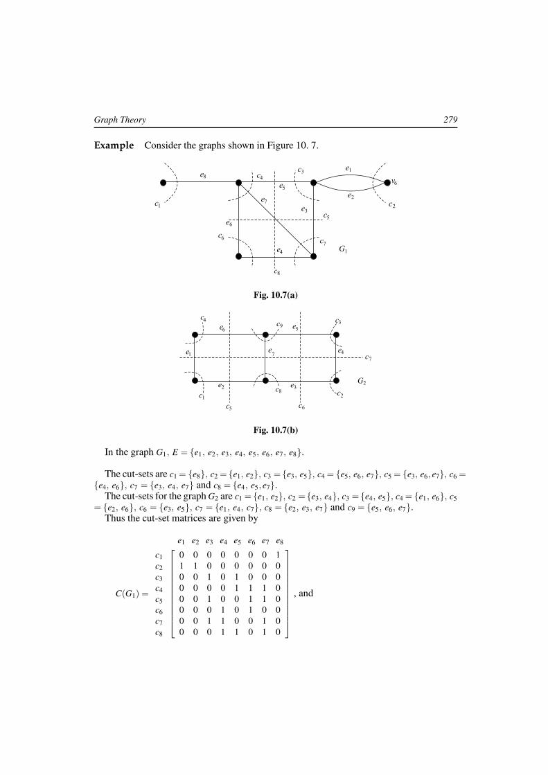
Example Consider the graphs shown in Figure 10. 7.

Fig. 10.7(a)

Fig. 10.7(b)

In the graph G1, E = {e1, e2, e3, e4, e5, e6, e7, e8}.

The cut-sets are c1 = {e8}, c2 = {e1, e2}, c3 = {e3, e5}, c4 = {e5, e6, e7}, c5 = {e3, e6,e7}, c6 ={e4, e6}, c7 = {e3, e4, e7} and c8 = {e4, e5,e7}.

The cut-sets for the graph G2 are c1 = {e1, e2}, c2 = {e3, e4}, c3 = {e4, e5}, c4 = {e1, e6}, c5

= {e2, e6}, c6 = {e3, e5}, c7 = {e1, e4, c7}, c8 = {e2, e3, e7} and c9 = {e5, e6, e7}.Thus the cut-set matrices are given by

e1 e2 e3 e4 e5 e6 e7 e8

C(G1) =

c1

c2

c3

c4

c5

c6

c7

c8

0 0 0 0 0 0 0 1

1 1 0 0 0 0 0 0

0 0 1 0 1 0 0 0

0 0 0 0 1 1 1 0

0 0 1 0 0 1 1 0

0 0 0 1 0 1 0 0

0 0 1 1 0 0 1 0

0 0 0 1 1 0 1 0

, and

280 Graph Matrices

e1 e2 e3 e4 e5 e6 e7

C(G2) =

c1

c2

c3

c4

c5

c6

c7

c8

c9

1 1 0 0 0 0 0

0 0 1 1 0 0 0

0 0 0 1 1 0 0

1 0 0 0 0 1 0

0 1 0 0 0 1 0

0 0 1 0 1 0 0

1 0 0 1 0 0 1

0 1 1 0 0 0 1

0 0 0 0 1 1 1

.

We have the following observations about the cut-set matrix C(G) of a graph G.

1. The permutation of rows or columns in a cut-set matrix corresponds simply to re-naming of the cut-sets and edges respectively.

2. Each row in C(G) is a cut-set vector.

3. A column with all zeros corresponds to an edge forming a self-loop.

4. Parallel edges form identical columns in the cut-set matrix.

5. In a non-separable graph, since every set of edges incident on a vertex is a cut-set,therefore every row of incidence matrix A(G) is included as a row in the cut-set matrixC(G). That is, for a non-separable graph G, C(G) contains A(G). For a separable graph,the incidence matrix of each block is contained in the cut-set matrix. For example, inthe graph G1 of Figure 10.7, the incidence matrix of the block {e3, e4, e5, e6, e7} isthe 4×5 submatrix of C, left after deleting rows c1, c2, c5, c8 and columns e1, e2, e8.

6. It follows from observation 5, that rank C(G)≥ rank A(G). Therefore, for a connectedgraph with n vertices, rank C(G) ≥ n−1.

The following result for connected graphs shows that cutset matrix, incidence matrixand the corresponding graph matrix have the same rank.

Theorem 10.14 If G is a connected graph, then the rank of a cut-set matrix C(G) is equalto the rank of incidence matrix A(G), which equals the rank of graph G.

Proof Let A(G), B(G) and C(G) be the incidence, cycle and cut-set matrix of the con-nected graph G. Then we have

rank C(G) ≥ n−1. (10.14.1)

Since the number of edges common to a cut-set and a cycle is always even, every rowin C is orthogonal to every row in B, provided the edges in both B and C are arranged in thesame order.

Graph Theory 281

Thus, BCT = CBT ≡ 0 (mod 2). (10.14.2)

Now, applying Sylvester’s theorem to equation (10.14.2), we have

rank B+ rank C ≤ m.

For a connected graph, we have rank B = m−n +1.

Therefore, rank C ≤ m− rank B = m− (m−n +1) = n−1.

So, rank C ≤ n−1. (10.14.3)

It follows from (10.14.1) and (10.14.3) that rank C = n−1. q

10.5 Fundamental Cut-Set Matrix

Let G be a connected graph with n vertices and m edges. The fundamental cut-set matrix C f

of G is an (n−1)×m submatrix of C such that the rows correspond to the set of fundamentalcut-sets with respect to some spanning tree. Clearly, a fundamental cut-set matrix C f canbe partitioned into two submatrices, one of which is an identity matrix In−1 of order n−1.We have

C f = [Cc : In−1],

where the last n−1 columns forming the identity matrix correspond to the n−1 branchesof the spanning tree and the first m−n +1 columns forming Cc correspond to the chords.

Example Consider the connected graphs G1 and G2 given in Figure 10.8. The spanningtree is shown with bold lines. The fundamental cut-sets of G1 are c1, c2, c3, c6 and c7 whilethe fundamental cut-sets of G2 are c1, c2, c3, c4 and c7.

Fig. 10.8

The fundamental cut-set matrix of G1 and G2, respectively are given by

282 Graph Matrices

e2 e3 e4 e1 e5 e6 e7 e8

C f =

1 0 0... 1 0 0 0 0

0 1 0... 0 1 0 0 0

0 0 1... 0 0 1 0 0

0 1 1... 0 0 0 1 0

0 0 0... 0 0 0 0 1

and

e1 e4 e2 e3 e5 e6 e7

C f =

c1

c2

c3

c4

c7

1 0... 1 0 0 0 0

0 1... 0 1 0 0 0

0 1... 0 0 1 0 0

1 0... 0 0 0 1 0

1 1... 0 0 0 0 1

10.6 Relations between A f , B f and C f

Let G be a connected graph and A f ,B f and C f be respectively the reduced incidence matrix,the fundamental cycle matrix, and the fundamental cut-set matrix of G.

We have shown that

B f =

[

Iµ

... Bt

]

(10.6.i)

and C f =

[

Cc

... In−1

]

, (10.6.ii)

where Bt denotes the submatrix corresponding to the branches of a spanning tree and Cc

denotes the submatrix corresponding to the chords.Let the spanning tree T in Equations (10.6.i) and (10.6.ii) be the same and let the order

of the edges in both equations be same. Also, in the reduced incidence matrix A f of size(n−1)×m, let the edges (i.e., the columns) be arranged in the same order as in B f and C f .

Partition A f into two submatrices given by

A f =

[

Ac

... At

]

, (10.6.iii)

where At consists of n− 1 columns corresponding to the branches of the spanning tree T

and Ac is the spanning submatrix corresponding to the m−n +1 chords.

Graph Theory 283

Since the columns in A f and B f are arranged in the same order, the equation ABT =BAT = 0(mod 2) gives

A f BTf ≡ 0(mod 2),

or

[

Ac

... At

]

Iµ

...BT

t

≡ 0(mod 2),

or Ac +At BTf ≡ 0(mod 2). (10.6.iv)

Since At is non singular, A−1t exists. Now, premultiplying both sides of equation (10.6.iv)

by A−1t , we have

A−1t Ac +A−1

t At BTt ≡ 0(mod 2),

or A−1t Ac +BT

t ≡ 0(mod 2).

Therefore, A−1t Ac = −BT

t .

Since in mod 2 arithmetic −1 = 1,

BTt = A−1

t Ac. (10.6.v)

Now as the columns in B f and C f are arranged in the same order, therefore (in mod 2arithmetic) C f . BT

f ≡ 0(mod 2) in mod 2 arithmetic gives C f .BTf = 0.

Therefore,

[

Cc

... In−1

]

Iµ

...BT

t

= 0, so that Cc +BT

t = 0, that is, Cc = −BTt .

Thus, Cc = BTt (as −1 = 1 in mod 2 arithmetic).

Hence, Cc = A−1t Ac from (10.6.v).

Remarks We make the following observations from the above relations.

1. If A or A f is given, we can construct B f and C f starting from an arbitrary spanningtree and its submatrix At in A f .

2. If either B f or C f is given, we can construct the other. Therefore, since B f determinesa graph within 2-isomorphism, so does C f .

3. If either B f and C f is given, then A f in general cannot be determined completely.

284 Graph Matrices

Example Consider the graph G of Figure 10.9.

Fig. 10.9

Let {e1, e5, e6, e7, e8} be the spanning tree.

e1 e2 e3 e4 e5 e6 e7 e8

We have, A =

0 0 0 1 0 1 0 0

0 0 0 0 1 1 1 1

0 0 0 0 0 0 0 1

1 1 1 0 1 0 0 0

0 0 1 1 0 0 1 0

1 1 0 0 0 0 0 0

.

Dropping the sixth row in A, we get

e2 e3 e4 e1 e5 e6 e7 e8

A f =

0 0 1 : 0 0 1 0 0

0 0 0 : 0 1 1 1 1

0 0 0 : 0 0 0 0 1

1 1 0 : 1 1 0 0 0

0 1 1 : 0 0 0 1 0

= [Ac : At ].

e2 e3 e4 e1 e5 e6 e7 e8

B f =

1 0 0 : 1 0 0 0

0 1 0 : 0 1 0 1

0 0 1 : 0 0 1 1

0

0

0

= [I3 : Bt ] and

Graph Theory 285

e2 e3 e4 e1 e5 e6 e7 e8

C f =

1 0 0 1 0 0 0 0

0 1 0 0 1 0 0 0

0 0 1 0 0 1 0 0

0 1 1 0 0 0 1 0

0 0 0 0 0 0 0 1

= [Cc : I5] .

Clearly, BTt = Cc.

We verify A−1t Ac = BT

t .

Now,

At =

0 0 1 0 0

0 1 1 1 1

0 0 0 0 1

1 1 0 0 0

0 0 0 1 0

,Bt =

1 0 0 0 0

0 1 0 1 0

0 0 1 1 0

Therefore, A−1t Ac =

1 0 0

0 1 0

0 0 1

0 1 1

0 0 0

. Hence, A−1t Ac = BT

t .

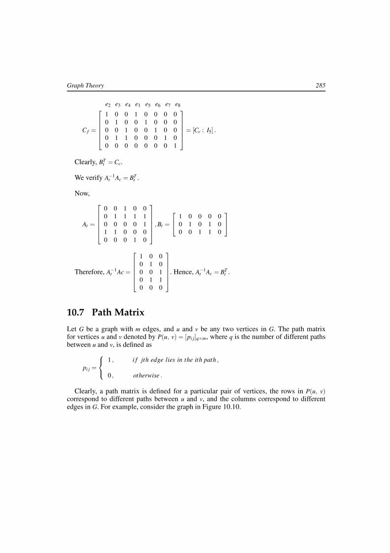
10.7 Path Matrix

Let G be a graph with m edges, and u and v be any two vertices in G. The path matrixfor vertices u and v denoted by P(u, v) = [pi j]q×m, where q is the number of different pathsbetween u and v, is defined as

pi j =

1 , i f jth edge lies in the ith path ,

0 , otherwise .

Clearly, a path matrix is defined for a particular pair of vertices, the rows in P(u, v)correspond to different paths between u and v, and the columns correspond to differentedges in G. For example, consider the graph in Figure 10.10.

286 Graph Matrices

Fig. 10.10

The different paths between the vertices v3 and v4 are

p1 = {e8, e5}, p2 = {e8, e7, e3} and p3 = {e8, e6, e4, e3}.

The path matrix for v3, v4 is given by

e1 e2 e3 e4 e5 e6 e7 e8

P(v3, v4) =

0 0 0 0 1 0 0 1

0 0 1 0 0 0 1 1

0 0 1 1 0 1 0 1

.

We have the following observations about the path matrix.

1. A column of all zeros corresponds to an edge that does not lie in any path between u

and v.

2. A column of all ones corresponds to an edge that lies in every path between u and v.

3. There is no row with all zeros.

4. The ring sum of any two rows in P(u, v) corresponds to a cycle or an edge-disjointunion of cycles.

The next result gives a relation between incidence and path matrix of a graph.

Theorem 10.15 If the columns of the incidence matrix A and the path matrix P(u, v)of a connected graph are arranged in the same order, then under the product (mod 2).

APT (u, v) = M,

where M is a matrix having ones in two rows u and v, and the zeros in the remaining n−2

rows.

Proof Let G be a connected graph and let vk = u and vt = v be any two vertices of G. LetA be the incidence matrix and P(u, v) be the path matrix of (u, v) in G.

Graph Theory 287

Now for any vertex vi in G and for any u− v path p j in G, either vi ∈ p j or vi /∈ p j.If vi /∈ p j, then there is no edge of p j which is incident on vi.If vi ∈ p j, then either vi is an intermediate vertex of p j , or vi = vk or vt . In case vi is an

intermediate vertex of p j, then there are exactly two edges of p j which are incident on vi

and in case vi = vk or vt , there is exactly one edge of p j which is incident on vi.Now consider the ith row of A and the jth row of P (which is the jth column of PT (u, v)).

As the edges are arranged in the same order, the rth entries in these two rows are bothnon zero if and only if the edge er is incident on the ith vertex vi and is also on the jth pathp j. Let APT (u, v) = M = [mi j].

We have,[

APT]

i j=

m

∑r=1

[A]ir[PT ]r j .

Therefore, mi j =m

∑r=1

air p jr.

For each edge er of G, we have one of the following cases.

i. er is incident on vi and er /∈ p j . Here air = 1,b jr = 0.

ii. er is not incident on vi and er ∈ p j. Here air = 0,b jr = 1.

iii. er is not incident on vi and er /∈ p j. Here air = 0,b jr = 0.

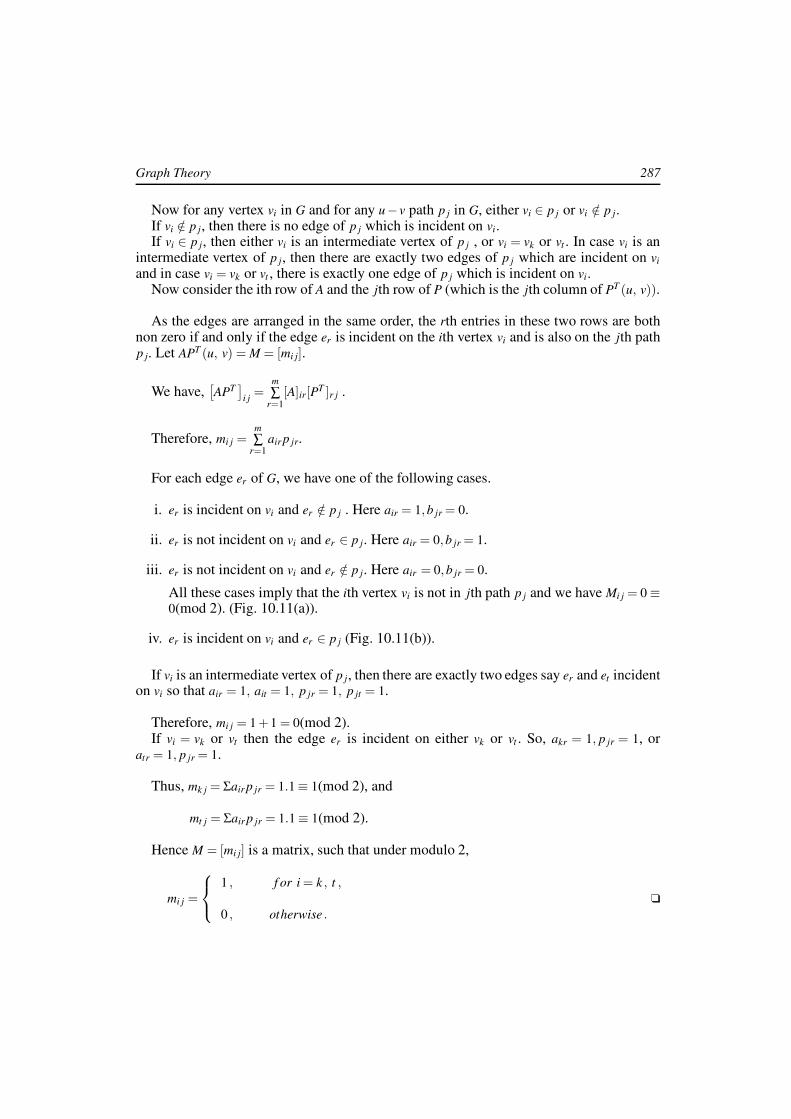
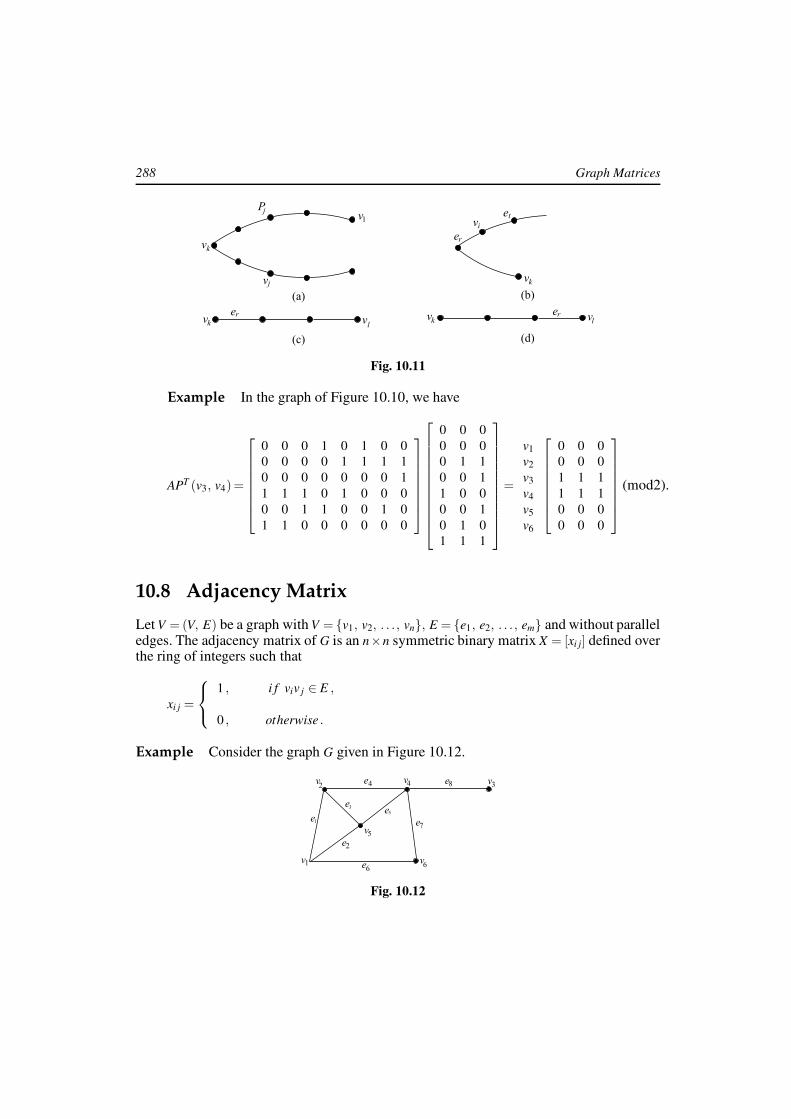
All these cases imply that the ith vertex vi is not in jth path p j and we have Mi j = 0 ≡0(mod 2). (Fig. 10.11(a)).

iv. er is incident on vi and er ∈ p j (Fig. 10.11(b)).

If vi is an intermediate vertex of p j, then there are exactly two edges say er and et incidenton vi so that air = 1, ait = 1, p jr = 1, p jt = 1.

Therefore, mi j = 1 +1 = 0(mod 2).If vi = vk or vt then the edge er is incident on either vk or vt . So, akr = 1, p jr = 1, or

atr = 1, p jr = 1.

Thus, mk j = Σair p jr = 1.1 ≡ 1(mod 2), and

mt j = Σair p jr = 1.1 ≡ 1(mod 2).

Hence M = [mi j] is a matrix, such that under modulo 2,

mi j =

1 , f or i = k , t ,

0 , otherwise .q

288 Graph Matrices

Fig. 10.11

Example In the graph of Figure 10.10, we have

APT (v3, v4)=

0 0 0 1 0 1 0 0

0 0 0 0 1 1 1 1

0 0 0 0 0 0 0 1

1 1 1 0 1 0 0 0

0 0 1 1 0 0 1 0

1 1 0 0 0 0 0 0

0 0 0

0 0 0

0 1 1

0 0 1

1 0 0

0 0 1

0 1 0

1 1 1

=

v1

v2

v3

v4

v5

v6

0 0 0

0 0 0

1 1 1

1 1 1

0 0 0

0 0 0

(mod2).

10.8 Adjacency Matrix

Let V = (V, E) be a graph with V = {v1, v2, . . . , vn}, E = {e1, e2, . . . , em} and without paralleledges. The adjacency matrix of G is an n×n symmetric binary matrix X = [xi j] defined overthe ring of integers such that

xi j =

1 , i f viv j ∈ E ,

0 , otherwise .

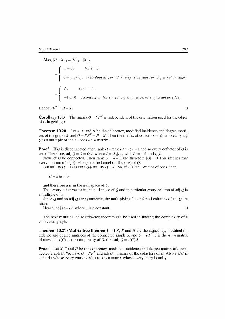
Example Consider the graph G given in Figure 10.12.

Fig. 10.12

Graph Theory 289

The adjacency matrix of G is given by

v1 v2 v3 v4 v5 v6

X =

v1

v2

v3

v4

v5

v6

0 1 0 0 1 1

1 0 0 1 1 0

0 0 0 1 0 0

0 1 1 0 1 0

1 1 0 1 0 0

1 0 0 1 0 0

.

We have the following observations about the adjacency matrix X of a graph G.

1. The entries along the principal diagonal of X are all zeros if and only if the graph hasno self-loops. However, a self-loop at the ith vertex corresponds to xii = 1.

2. If the graph has no self-loops, the degree of a vertex equals the number of ones in thecorresponding row or column of X .

3. Permutation of rows and the corresponding columns imply reordering the vertices.We note that the rows and columns are arranged in the same order. Therefore, whentwo rows are interchanged in X , the corresponding columns are also interchanged.Thus two graphs G1 and G2 without parallel edges are isomorphic if and only if theiradjacency matrices X(G1) and X(G2) are related by

X(G2) = R−1X(G1)R,

where R is a permutation matrix.

4. A graph G is disconnected having components G1 and G2 if and only if the adjacencymatrix X(G) is partitioned as

X(G) =

X(G1) : O

. . : . .O : X(G2)

,

where X(G1) and X(G2) are respectively the adjacency matrices of the componentsG1 and G2. Obviously, the above partitioning implies that there are no edges betweenvertices in G1 and vertices in G2.

5. If any square, symmetric and binary matrix Q of order n is given, then there exists agraph G with n vertices and without parallel edges whose adjacency matrix is Q.

Definition: An edge sequence is a sequence of edges in which each edge, except thefirst and the last, has one vertex in common with the edge preceding it and one vertex

290 Graph Matrices

in common with the edge following it. A walk and a path are the examples of an edgesequence. An edge can appear more than once in an edge sequence. In the graph of Figure10.13, v1e1v2e2v3e3v4e4v2e2v3e5v5, or e1e2e3e4e2e5 is an edge sequence.

Fig. 10.13

We now have the following result.

Theorem 10.16 If X = [xi j] is the adjacency matrix of a simple graph G, then [Xk]i j isthe number of different edge sequences of length k between vertices vi and v j .

Proof We prove the result by using induction on k. The result is trivial for k = 0 and 1.Since X2 = X .X , X2 is a symmetric matrix, as product of symmetric matrices is also

symmetric.

For k = 2, i 6= j, we have

[X2]i j = number of ones in the product of ith row and jth column (or jth row) of X

= number of positions in which both ith and jth rows of X have ones

= number of vertices that are adjacent to both ith and jth vertices

= number of different paths of length two between ith and jth vertices

Also, [X2]ii = number of ones in the ith row (or column) of X

= degree of the corresponding vertex.

This shows that [X2]i j is the number of different paths and therefore different edge se-quences of length 2 between the vertices vi and v j. Thus the result is true for k = 2.

Assume the result to be true for k, so that

[Xk]i j= number of different edge sequences of length k between vi and v j .

We have, [Xk+1]i j = [XkX ]i j =n

∑r=1

[Xk]ir[X ]r j=

n

∑r=1

[Xk]irxr j.

Graph Theory 291

Now, every vi − v j edge sequence of length k + 1 consists of a vi − vr edge sequence oflength k, followed by an edge vtv j . Since there are [Xk]ir such edge sequences of lengthk and xr j such edges for each vertex vr, the total number of all vi − v j edge sequences of

length k+1 isn

∑r=1

[Xk]irxr j. This proves the result for k+1 also. q

We have the following observation about connectedness and adjacency matrix.

Theorem 10.17 Let G be a graph with V = {v1, v2, . . ., vn} and let X be the adjacencymatrix of G. Let Y = [yi j] be the matrix Y = X +X2 + . . .+Xn−1.

Then G is connected if and only if for all distinct i, j, yi j 6= 0. That is, if and only if Y hasno zero entries off the main diagonal.

Proof We have, yi j = [Y ]i j = [X ]i j +[X2]i j + . . .+[Xn−1]i j.

Since [Xk]i j denotes the number of distinct edge-sequences of length k from vi to v j ,

yi j = number of different vi − v j edge sequence of length 1

+ number of different vi − v j edge sequences of length 2 + . . .

+ number of different vi − v j edge sequences of length n−1.

Therefore, yi j = number of different vi − v j edge sequence of length less than n.

Now let G be connected. Then for every pair of distinct i, j there is a path from vi tov j. Since G has n vertices, this path passes through atmost n vertices and so has length lessthan n. Thus, yi j 6= 0 for each i, j with i 6= j.

Conversely, for each distinct pair i, j we have yi j 6= 0. Then from above, there is at leastone edge sequence of length less than n from vi to v j. This implies that vi is connected tov j. Since the distinct pair i, j is chosen arbitrarily, G is connected. q

The next result is useful in determining the distances between different pairs of vertices.

Theorem 10.18 In a connected graph, the distance between two vertices vi and v j is k ifand only if k is the smallest integer for which [Xk]i j 6= 0.

Proof Let G be a connected graph and let X = [xi j] be the adjacency matrix of G. Let vi

and v j be vertices in G such that

d(vi, v j) = k.

Then the length of the shortest path between vi and v j is k.

This implies that there are no paths of length 1, 2, . . ., k−1 and so no edge sequences oflength 1, 2, . . . , k−1 between vi and v j .

292 Graph Matrices

Therefore, [X ]i j = 0, [X2]i j = 0, . . ., [Xk−1]i j = 0.

Hence k is the smallest integer such that [Xk]i j 6= 0.

Conversely, suppose that k is the smallest integer such that [Xk]i j 6= 0.

Therefore, there are no edge sequences of length 1, 2, . . ., k−1 and in fact no paths oflength 1, 2, . . . , k−1 between vertices vi and v j .

Thus the shortest path between vi and v j is of length k, so that d(vi, v j) = k. q

Definition: Let G be a graph and let di be the degree of the vertex vi in G. The degreematrix H = [hi j] of G is defined by

hi j =

0 , f or i 6= j ,

di , f or i = j .

The following result gives a relation between the matrices F,X and H.

Theorem 10.19 Let F be the modified incidence matrix, X the adjacency matrix and H

the degree matrix of a graph G. Then

FFT = H −X .

Proof We have (i, j)th element of FFT ,

[FFT ]i j =m

∑r=1

[F]ir[FT ]r j =

m

∑r=1

[F ]ir[F ] jr.

Now, [F]ir and [F]r j are non-zero if and only if the edge er = viv j. Then for i 6= j,

m

∑r=1

[F]ir[F ] jr =

−1 , i f er = viv j is an edge ,

0 , i f er = viv j is not an edge .

For i = j, [F]ir[F] jr = 1 whenever [F]ik = ±1, and this occurs di times corresponding tothe number of edges incident on vi. Thus,

m

∑r=1

[F]ir[F ] jr = di, for i = j.

Therefore,

[FFT ]i j =

−1 or 0 , according to whether f or i 6= j , viv j is an edge or not ,

di , f or i = j .

Graph Theory 293

Also, [H −X ]i j = [H]i j− [X ]i j

=

di −0 , f or i = j ,

0− (1 or 0) , according as f or i 6= j , viv j is an edge, or viv j is not an edge .

=

di , f or i = j ,

−1 or 0 , according as f or i 6= j , viv j is an edge, or viv j is not an edge .

Hence FFT = H −X . q

Corollary 10.3 The matrix Q = FFT is independent of the orientation used for the edgesof G in getting F.

Theorem 10.20 Let X , F and H be the adjacency, modified incidence and degree matri-ces of the graph G, and Q = FFT = H −X . Then the matrix of cofactors of Q denoted by adjQ is a multiple of the all ones n×n matrix J.

Proof If G is disconnected, then rank Q =rank FFT < n−1 and so every cofactor of Q iszero. Therefore, adj Q = O = O.J, where J = [Ji j]n×n with Ji j = 1 for all i, j.

Now let G be connected. Then rank Q = n− 1 and therefore |Q| = 0 This implies thatevery column of adj Q belongs to the kernel (null space) of Q.

But nullity Q = 1 (as rank Q+ nullity Q = n). So, if u is the n-vector of ones, then

(H −X)u = 0.

and therefore u is in the null space of Q.Thus every other vector in the null space of Q and in particular every column of adj Q is

a multiple of u.Since Q and so adj Q are symmetric, the multiplying factor for all columns of adj Q are

same.Hence, adj Q = cJ, where c is a constant. q

The next result called Matrix-tree theorem can be used in finding the complexity of aconnected graph.

Theorem 10.21 (Matrix-tree theorem) If X , F and H are the adjacency, modified in-cidence and degree matrices of the connected graph G, and Q = FFT ,J is the n×n matrixof ones and τ(G) is the complexity of G, then adj Q = τ(G).J.

Proof Let X ,F and H be the adjacency, modified incidence and degree matrix of a con-nected graph G. We have Q = FFT and adj Q = matrix of the cofactors of Q. Also τ(G)J isa matrix whose every entry is τ(G) as J is a matrix whose every entry is unity.

294 Graph Matrices

Therefore, to prove adj Q = τ(G)J, it is enough to prove that τ(G) = any one cofactor ofQ.

Let F0 be the matrix obtained by dropping the last row from F. Then clearly, |FoFTo | is a

cofactor of Q.Using Binet-Cauchy theorem of matrix theory, we have

∣

∣F0FT0

∣

∣ = ∑X⊆E

|Fx |∣

∣FTx

∣

∣ , (10.21.1)

where Fx is the square submatrix of Fo whose n− 1 columns correspond to n− 1 edges inthe subset X of E, the summation running over all possible such subsets.

We know |Fx| 6= 0 if and only if < X > is a spanning tree of G and |Fx| = ±1.But, |FT

x |= |Fx| .Therefore each X ⊆ E such that < X > is a spanning tree of G contributes one to the sum

on the right of (10.21.1) and all other contributions are zero.Hence |FoFT

o | = τ(G), proving the theorem. q

Corollary 10.4 Prove τ(Kn) = nn−2.

Proof Here, Q = H −X = (n−1)I − (J− I) = nI− J . Therefore,

Q =

n 0 0 . . 0

0 n 0 . . 0

0 0 n . . 0

:

0 0 0 . . n

−

1 1 1 . . 1

1 1 1 . . 1

1 1 1 . . 1

:

1 1 1 . . 1

=

n−1 −1 −1 . . −1

−1 n−1 −1 . . −1

−1 −1 n−1 . . −1

:

−1 −1 −1 . . n−1

.

The cofactor of q11 is the (n−1)× (n−1) determinant given by

cofactor of q11 =

∣

∣

∣

∣

∣

∣

∣

∣

n−1 −1 . . −1

−1 n−1 . . −1

:

−1 −1 . . n−1

∣

∣

∣

∣

∣

∣

∣

∣

.

Subtracting the first row from each of the others and then adding the last n−2 columnsto the first, we get

Graph Theory 295

cofactor of q11 =

∣

∣

∣

∣

∣

∣

∣

∣

∣

∣

1 −1 −1 . . −1

0 n 0 . . 0

0 0 n . . 0

:

0 0 0 . . n

∣

∣

∣

∣

∣

∣

∣

∣

∣

∣

.

Expanding with the help of the first column, we have cofactor of q11 = nn−2. Thus,

τ(kn) = nn−2. q

10.9 Exercises

1. Characterise A f , B f , C f and X of the complete graph of n vertices.

2. Characterise simple, self-dual graphs in terms of their cycle and cut-set matrices.

3. Show that each diagonal entry in X3 equals twice the number of triangles passingthrough the corresponding vertex.

4. Characterise the adjacency matrix of a bipartite graph.

5. Prove that a graph is bipartite if and only if for all odd k, every diagonal entry of Ak

is zero.

6. Similar to the cycle or cut-set matrix, define a spanning tree matrix for a connectedgraph, and observe some of its properties.

7. If X is the adjacency matrix of a graph G and L is the adjacency matrix of its edgegraph L(G) and A and H are the incidence and degree matrices, show that X = AAT −H

and L = AT A−2I.

8. Use the matrix tree theorem to calculate τ(K4 − e).

9. Prove that τ(G) =1

n2det(J +Q).