1/2/2016 10 Minutes to pandas — pandas 0.17.1 documentation

http://pandas.pydata.org/pandas-docs/stable/10min.html 1/26

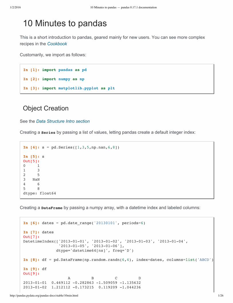
10 Minutes to pandasThis is a short introduction to pandas, geared mainly for new users. You can see more complexrecipes in the Cookbook

Customarily, we import as follows:

In [1]: import pandas as pd

In [2]: import numpy as np

In [3]: import matplotlib.pyplot as plt

Object Creation

See the Data Structure Intro section

Creating a Series by passing a list of values, letting pandas create a default integer index:

In [4]: s = pd.Series([1,3,5,np.nan,6,8])

In [5]: s Out[5]: 0 1 1 3 2 5 3 NaN 4 6 5 8 dtype: float64

Creating a DataFrame by passing a numpy array, with a datetime index and labeled columns:

In [6]: dates = pd.date_range('20130101', periods=6)

In [7]: dates Out[7]: DatetimeIndex(['2013-01-01', '2013-01-02', '2013-01-03', '2013-01-04', '2013-01-05', '2013-01-06'], dtype='datetime64[ns]', freq='D')

In [8]: df = pd.DataFrame(np.random.randn(6,4), index=dates, columns=list('ABCD'))

In [9]: df Out[9]: A B C D 2013-01-01 0.469112 -0.282863 -1.509059 -1.135632 2013-01-02 1.212112 -0.173215 0.119209 -1.044236

1/2/2016 10 Minutes to pandas — pandas 0.17.1 documentation

http://pandas.pydata.org/pandas-docs/stable/10min.html 2/26

Creating a DataFrame by passing a dict of objects that can be converted to series­like.

Having specific dtypes

In [12]: df2.dtypes Out[12]: A float64 B datetime64[ns] C float32 D int32 E category F object dtype: object

If you’re using IPython, tab completion for column names (as well as public attributes) isautomatically enabled. Here’s a subset of the attributes that will be completed:

In [13]: df2.<TAB> df2.A df2.boxplot df2.abs df2.C df2.add df2.clip df2.add_prefix df2.clip_lower df2.add_suffix df2.clip_upper df2.align df2.columns df2.all df2.combine df2.any df2.combineAdd df2.append df2.combine_first df2.apply df2.combineMult df2.applymap df2.compound df2.as_blocks df2.consolidate df2.asfreq df2.convert_objects df2.as_matrix df2.copy

2013-01-03 -0.861849 -2.104569 -0.494929 1.071804 2013-01-04 0.721555 -0.706771 -1.039575 0.271860 2013-01-05 -0.424972 0.567020 0.276232 -1.087401 2013-01-06 -0.673690 0.113648 -1.478427 0.524988

In [10]: df2 = pd.DataFrame( 'A' : 1., ....: 'B' : pd.Timestamp('20130102'), ....: 'C' : pd.Series(1,index=list(range(4)),dtype='float32' ....: 'D' : np.array([3] * 4,dtype='int32'), ....: 'E' : pd.Categorical(["test","train","test","train" ....: 'F' : 'foo' ) ....:

In [11]: df2 Out[11]: A B C D E F 0 1 2013-01-02 1 3 test foo 1 1 2013-01-02 1 3 train foo 2 1 2013-01-02 1 3 test foo 3 1 2013-01-02 1 3 train foo

1/2/2016 10 Minutes to pandas — pandas 0.17.1 documentation

http://pandas.pydata.org/pandas-docs/stable/10min.html 3/26

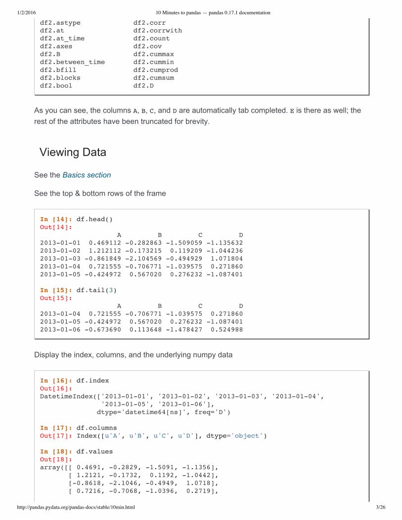
df2.astype df2.corr df2.at df2.corrwith df2.at_time df2.count df2.axes df2.cov df2.B df2.cummax df2.between_time df2.cummin df2.bfill df2.cumprod df2.blocks df2.cumsum df2.bool df2.D

As you can see, the columns A, B, C, and D are automatically tab completed. E is there as well; therest of the attributes have been truncated for brevity.

Viewing Data

See the Basics section

See the top & bottom rows of the frame

In [14]: df.head() Out[14]: A B C D 2013-01-01 0.469112 -0.282863 -1.509059 -1.135632 2013-01-02 1.212112 -0.173215 0.119209 -1.044236 2013-01-03 -0.861849 -2.104569 -0.494929 1.071804 2013-01-04 0.721555 -0.706771 -1.039575 0.271860 2013-01-05 -0.424972 0.567020 0.276232 -1.087401

In [15]: df.tail(3) Out[15]: A B C D 2013-01-04 0.721555 -0.706771 -1.039575 0.271860 2013-01-05 -0.424972 0.567020 0.276232 -1.087401 2013-01-06 -0.673690 0.113648 -1.478427 0.524988

Display the index, columns, and the underlying numpy data

In [16]: df.index Out[16]: DatetimeIndex(['2013-01-01', '2013-01-02', '2013-01-03', '2013-01-04', '2013-01-05', '2013-01-06'], dtype='datetime64[ns]', freq='D')

In [17]: df.columns Out[17]: Index([u'A', u'B', u'C', u'D'], dtype='object')

In [18]: df.values Out[18]: array([[ 0.4691, -0.2829, -1.5091, -1.1356], [ 1.2121, -0.1732, 0.1192, -1.0442], [-0.8618, -2.1046, -0.4949, 1.0718], [ 0.7216, -0.7068, -1.0396, 0.2719],

1/2/2016 10 Minutes to pandas — pandas 0.17.1 documentation

http://pandas.pydata.org/pandas-docs/stable/10min.html 4/26

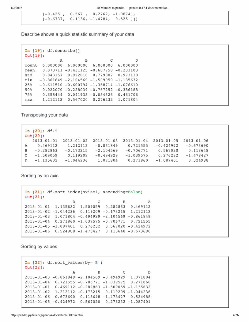
Describe shows a quick statistic summary of your data

In [19]: df.describe() Out[19]: A B C D count 6.000000 6.000000 6.000000 6.000000 mean 0.073711 -0.431125 -0.687758 -0.233103 std 0.843157 0.922818 0.779887 0.973118 min -0.861849 -2.104569 -1.509059 -1.135632 25% -0.611510 -0.600794 -1.368714 -1.076610 50% 0.022070 -0.228039 -0.767252 -0.386188 75% 0.658444 0.041933 -0.034326 0.461706 max 1.212112 0.567020 0.276232 1.071804

Transposing your data

Sorting by an axis

In [21]: df.sort_index(axis=1, ascending=False) Out[21]: D C B A 2013-01-01 -1.135632 -1.509059 -0.282863 0.469112 2013-01-02 -1.044236 0.119209 -0.173215 1.212112 2013-01-03 1.071804 -0.494929 -2.104569 -0.861849 2013-01-04 0.271860 -1.039575 -0.706771 0.721555 2013-01-05 -1.087401 0.276232 0.567020 -0.424972 2013-01-06 0.524988 -1.478427 0.113648 -0.673690

Sorting by values

In [22]: df.sort_values(by='B') Out[22]: A B C D 2013-01-03 -0.861849 -2.104569 -0.494929 1.071804 2013-01-04 0.721555 -0.706771 -1.039575 0.271860 2013-01-01 0.469112 -0.282863 -1.509059 -1.135632 2013-01-02 1.212112 -0.173215 0.119209 -1.044236 2013-01-06 -0.673690 0.113648 -1.478427 0.524988 2013-01-05 -0.424972 0.567020 0.276232 -1.087401

[-0.425 , 0.567 , 0.2762, -1.0874], [-0.6737, 0.1136, -1.4784, 0.525 ]])

In [20]: df.T Out[20]: 2013-01-01 2013-01-02 2013-01-03 2013-01-04 2013-01-05 2013-01-06 A 0.469112 1.212112 -0.861849 0.721555 -0.424972 -0.673690 B -0.282863 -0.173215 -2.104569 -0.706771 0.567020 0.113648 C -1.509059 0.119209 -0.494929 -1.039575 0.276232 -1.478427 D -1.135632 -1.044236 1.071804 0.271860 -1.087401 0.524988

1/2/2016 10 Minutes to pandas — pandas 0.17.1 documentation

http://pandas.pydata.org/pandas-docs/stable/10min.html 5/26

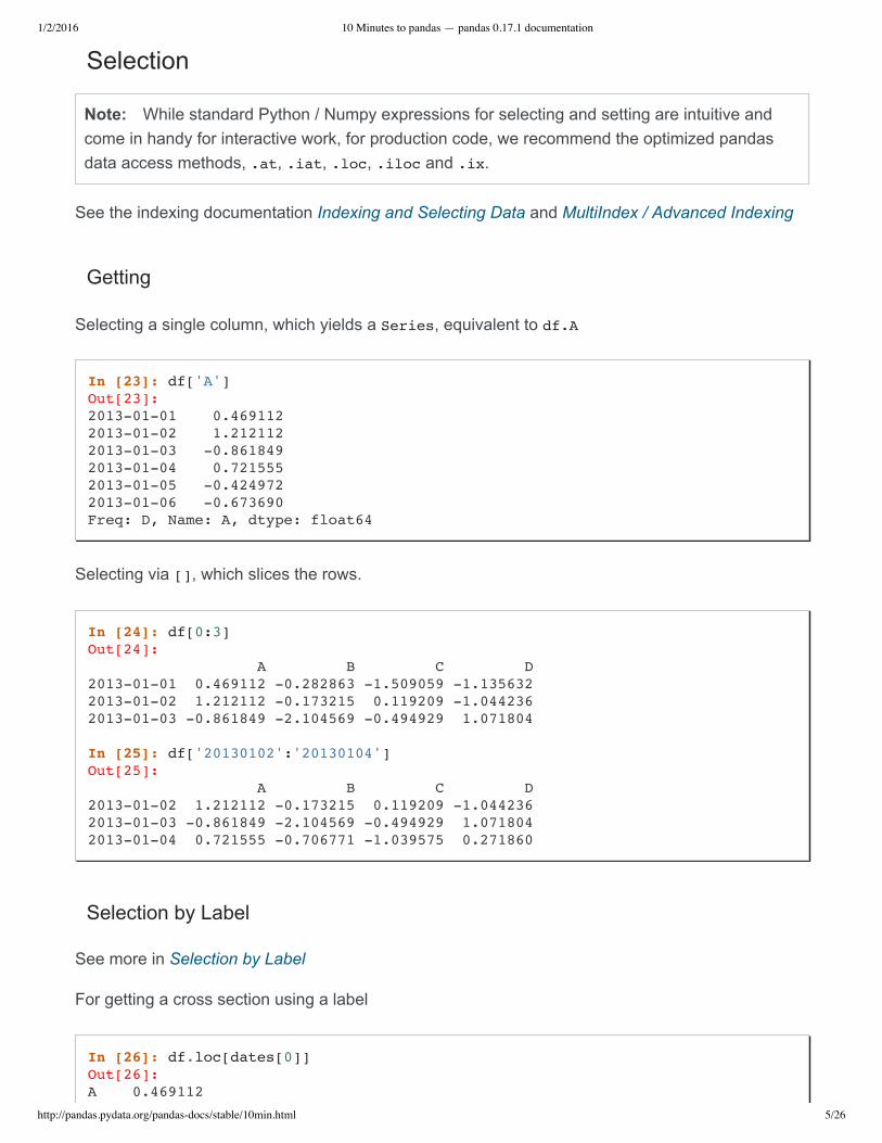
Selection

Note: While standard Python / Numpy expressions for selecting and setting are intuitive andcome in handy for interactive work, for production code, we recommend the optimized pandasdata access methods, .at, .iat, .loc, .iloc and .ix.

See the indexing documentation Indexing and Selecting Data and MultiIndex / Advanced Indexing

Getting

Selecting a single column, which yields a Series, equivalent to df.A

In [23]: df['A'] Out[23]: 2013-01-01 0.469112 2013-01-02 1.212112 2013-01-03 -0.861849 2013-01-04 0.721555 2013-01-05 -0.424972 2013-01-06 -0.673690 Freq: D, Name: A, dtype: float64

Selecting via [], which slices the rows.

In [24]: df[0:3] Out[24]: A B C D 2013-01-01 0.469112 -0.282863 -1.509059 -1.135632 2013-01-02 1.212112 -0.173215 0.119209 -1.044236 2013-01-03 -0.861849 -2.104569 -0.494929 1.071804

In [25]: df['20130102':'20130104'] Out[25]: A B C D 2013-01-02 1.212112 -0.173215 0.119209 -1.044236 2013-01-03 -0.861849 -2.104569 -0.494929 1.071804 2013-01-04 0.721555 -0.706771 -1.039575 0.271860

Selection by Label

See more in Selection by Label

For getting a cross section using a label

In [26]: df.loc[dates[0]] Out[26]: A 0.469112

1/2/2016 10 Minutes to pandas — pandas 0.17.1 documentation

http://pandas.pydata.org/pandas-docs/stable/10min.html 6/26

B -0.282863 C -1.509059 D -1.135632 Name: 2013-01-01 00:00:00, dtype: float64

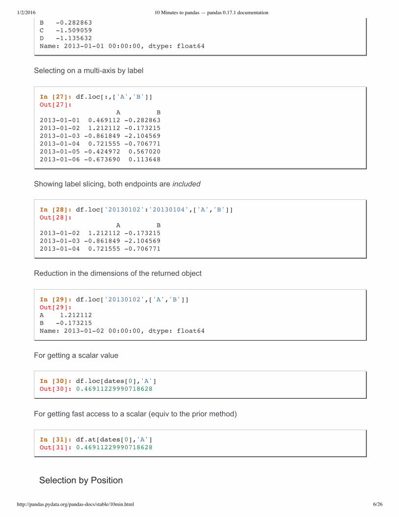
Selecting on a multi­axis by label

In [27]: df.loc[:,['A','B']] Out[27]: A B 2013-01-01 0.469112 -0.282863 2013-01-02 1.212112 -0.173215 2013-01-03 -0.861849 -2.104569 2013-01-04 0.721555 -0.706771 2013-01-05 -0.424972 0.567020 2013-01-06 -0.673690 0.113648

Showing label slicing, both endpoints are included

In [28]: df.loc['20130102':'20130104',['A','B']] Out[28]: A B 2013-01-02 1.212112 -0.173215 2013-01-03 -0.861849 -2.104569 2013-01-04 0.721555 -0.706771

Reduction in the dimensions of the returned object

In [29]: df.loc['20130102',['A','B']] Out[29]: A 1.212112 B -0.173215 Name: 2013-01-02 00:00:00, dtype: float64

For getting a scalar value

In [30]: df.loc[dates[0],'A'] Out[30]: 0.46911229990718628

For getting fast access to a scalar (equiv to the prior method)

In [31]: df.at[dates[0],'A'] Out[31]: 0.46911229990718628

Selection by Position

1/2/2016 10 Minutes to pandas — pandas 0.17.1 documentation

http://pandas.pydata.org/pandas-docs/stable/10min.html 7/26

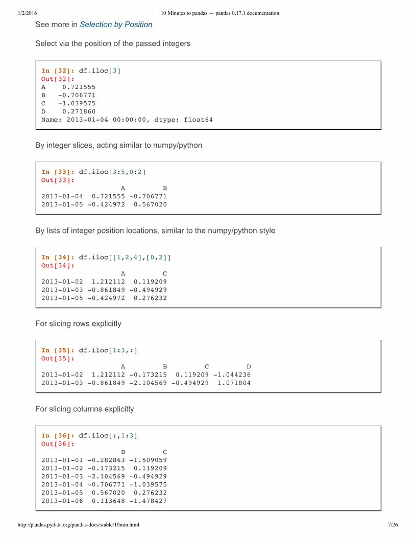
See more in Selection by Position

Select via the position of the passed integers

In [32]: df.iloc[3] Out[32]: A 0.721555 B -0.706771 C -1.039575 D 0.271860 Name: 2013-01-04 00:00:00, dtype: float64

By integer slices, acting similar to numpy/python

In [33]: df.iloc[3:5,0:2] Out[33]: A B 2013-01-04 0.721555 -0.706771 2013-01-05 -0.424972 0.567020

By lists of integer position locations, similar to the numpy/python style

In [34]: df.iloc[[1,2,4],[0,2]] Out[34]: A C 2013-01-02 1.212112 0.119209 2013-01-03 -0.861849 -0.494929 2013-01-05 -0.424972 0.276232

For slicing rows explicitly

In [35]: df.iloc[1:3,:] Out[35]: A B C D 2013-01-02 1.212112 -0.173215 0.119209 -1.044236 2013-01-03 -0.861849 -2.104569 -0.494929 1.071804

For slicing columns explicitly

In [36]: df.iloc[:,1:3] Out[36]: B C 2013-01-01 -0.282863 -1.509059 2013-01-02 -0.173215 0.119209 2013-01-03 -2.104569 -0.494929 2013-01-04 -0.706771 -1.039575 2013-01-05 0.567020 0.276232 2013-01-06 0.113648 -1.478427

1/2/2016 10 Minutes to pandas — pandas 0.17.1 documentation

http://pandas.pydata.org/pandas-docs/stable/10min.html 8/26

For getting a value explicitly

In [37]: df.iloc[1,1] Out[37]: -0.17321464905330858

For getting fast access to a scalar (equiv to the prior method)

In [38]: df.iat[1,1] Out[38]: -0.17321464905330858

Boolean Indexing

Using a single column’s values to select data.

In [39]: df[df.A > 0] Out[39]: A B C D 2013-01-01 0.469112 -0.282863 -1.509059 -1.135632 2013-01-02 1.212112 -0.173215 0.119209 -1.044236 2013-01-04 0.721555 -0.706771 -1.039575 0.271860

A where operation for getting.

In [40]: df[df > 0] Out[40]: A B C D 2013-01-01 0.469112 NaN NaN NaN 2013-01-02 1.212112 NaN 0.119209 NaN 2013-01-03 NaN NaN NaN 1.071804 2013-01-04 0.721555 NaN NaN 0.271860 2013-01-05 NaN 0.567020 0.276232 NaN 2013-01-06 NaN 0.113648 NaN 0.524988

Using the isin() method for filtering:

In [41]: df2 = df.copy()

In [42]: df2['E'] = ['one', 'one','two','three','four','three']

In [43]: df2 Out[43]: A B C D E 2013-01-01 0.469112 -0.282863 -1.509059 -1.135632 one 2013-01-02 1.212112 -0.173215 0.119209 -1.044236 one 2013-01-03 -0.861849 -2.104569 -0.494929 1.071804 two 2013-01-04 0.721555 -0.706771 -1.039575 0.271860 three 2013-01-05 -0.424972 0.567020 0.276232 -1.087401 four 2013-01-06 -0.673690 0.113648 -1.478427 0.524988 three

1/2/2016 10 Minutes to pandas — pandas 0.17.1 documentation

http://pandas.pydata.org/pandas-docs/stable/10min.html 9/26

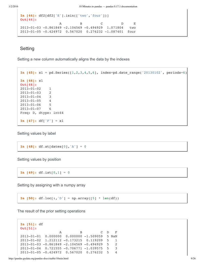
Setting

Setting a new column automatically aligns the data by the indexes

Setting values by label

In [48]: df.at[dates[0],'A'] = 0

Setting values by position

In [49]: df.iat[0,1] = 0

Setting by assigning with a numpy array

In [50]: df.loc[:,'D'] = np.array([5] * len(df))

The result of the prior setting operations

In [51]: df Out[51]: A B C D F 2013-01-01 0.000000 0.000000 -1.509059 5 NaN 2013-01-02 1.212112 -0.173215 0.119209 5 1 2013-01-03 -0.861849 -2.104569 -0.494929 5 2 2013-01-04 0.721555 -0.706771 -1.039575 5 3 2013-01-05 -0.424972 0.567020 0.276232 5 4

In [44]: df2[df2['E'].isin(['two','four'])] Out[44]: A B C D E 2013-01-03 -0.861849 -2.104569 -0.494929 1.071804 two 2013-01-05 -0.424972 0.567020 0.276232 -1.087401 four

In [45]: s1 = pd.Series([1,2,3,4,5,6], index=pd.date_range('20130102', periods=6))

In [46]: s1 Out[46]: 2013-01-02 1 2013-01-03 2 2013-01-04 3 2013-01-05 4 2013-01-06 5 2013-01-07 6 Freq: D, dtype: int64

In [47]: df['F'] = s1

1/2/2016 10 Minutes to pandas — pandas 0.17.1 documentation

http://pandas.pydata.org/pandas-docs/stable/10min.html 10/26

2013-01-06 -0.673690 0.113648 -1.478427 5 5

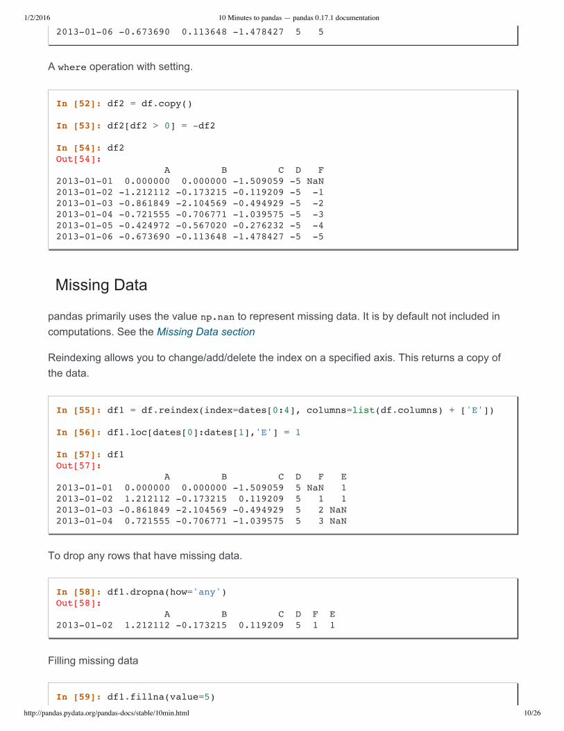
A where operation with setting.

In [52]: df2 = df.copy()

In [53]: df2[df2 > 0] = -df2

In [54]: df2 Out[54]: A B C D F 2013-01-01 0.000000 0.000000 -1.509059 -5 NaN 2013-01-02 -1.212112 -0.173215 -0.119209 -5 -1 2013-01-03 -0.861849 -2.104569 -0.494929 -5 -2 2013-01-04 -0.721555 -0.706771 -1.039575 -5 -3 2013-01-05 -0.424972 -0.567020 -0.276232 -5 -4 2013-01-06 -0.673690 -0.113648 -1.478427 -5 -5

Missing Data

pandas primarily uses the value np.nan to represent missing data. It is by default not included incomputations. See the Missing Data section

Reindexing allows you to change/add/delete the index on a specified axis. This returns a copy ofthe data.

To drop any rows that have missing data.

In [58]: df1.dropna(how='any') Out[58]: A B C D F E 2013-01-02 1.212112 -0.173215 0.119209 5 1 1

Filling missing data

In [59]: df1.fillna(value=5)

In [55]: df1 = df.reindex(index=dates[0:4], columns=list(df.columns) + ['E'])

In [56]: df1.loc[dates[0]:dates[1],'E'] = 1

In [57]: df1 Out[57]: A B C D F E 2013-01-01 0.000000 0.000000 -1.509059 5 NaN 1 2013-01-02 1.212112 -0.173215 0.119209 5 1 1 2013-01-03 -0.861849 -2.104569 -0.494929 5 2 NaN 2013-01-04 0.721555 -0.706771 -1.039575 5 3 NaN

1/2/2016 10 Minutes to pandas — pandas 0.17.1 documentation

http://pandas.pydata.org/pandas-docs/stable/10min.html 11/26

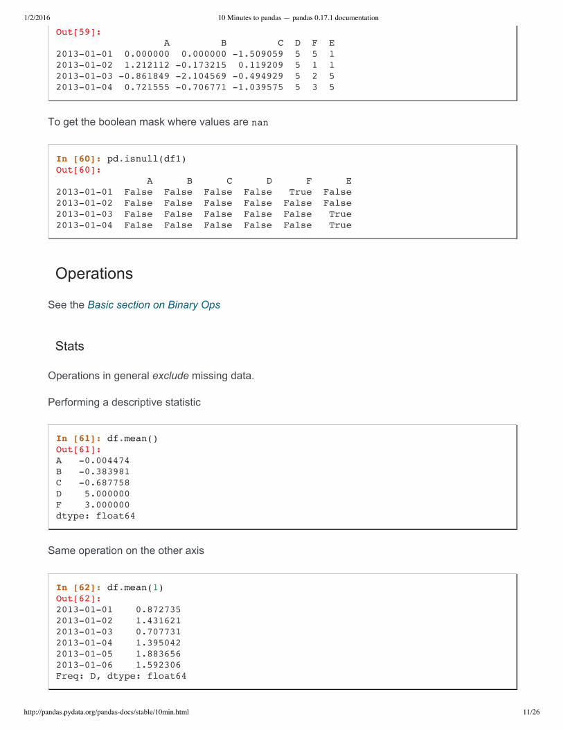
Out[59]: A B C D F E 2013-01-01 0.000000 0.000000 -1.509059 5 5 1 2013-01-02 1.212112 -0.173215 0.119209 5 1 1 2013-01-03 -0.861849 -2.104569 -0.494929 5 2 5 2013-01-04 0.721555 -0.706771 -1.039575 5 3 5

To get the boolean mask where values are nan

In [60]: pd.isnull(df1) Out[60]: A B C D F E 2013-01-01 False False False False True False 2013-01-02 False False False False False False 2013-01-03 False False False False False True 2013-01-04 False False False False False True

Operations

See the Basic section on Binary Ops

Stats

Operations in general exclude missing data.

Performing a descriptive statistic

In [61]: df.mean() Out[61]: A -0.004474 B -0.383981 C -0.687758 D 5.000000 F 3.000000 dtype: float64

Same operation on the other axis

In [62]: df.mean(1) Out[62]: 2013-01-01 0.872735 2013-01-02 1.431621 2013-01-03 0.707731 2013-01-04 1.395042 2013-01-05 1.883656 2013-01-06 1.592306 Freq: D, dtype: float64

1/2/2016 10 Minutes to pandas — pandas 0.17.1 documentation

http://pandas.pydata.org/pandas-docs/stable/10min.html 12/26

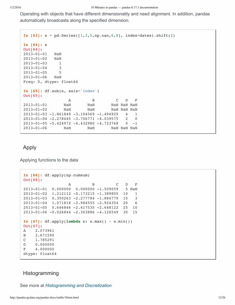
Operating with objects that have different dimensionality and need alignment. In addition, pandasautomatically broadcasts along the specified dimension.

Apply

Applying functions to the data

In [66]: df.apply(np.cumsum) Out[66]: A B C D F 2013-01-01 0.000000 0.000000 -1.509059 5 NaN 2013-01-02 1.212112 -0.173215 -1.389850 10 1 2013-01-03 0.350263 -2.277784 -1.884779 15 3 2013-01-04 1.071818 -2.984555 -2.924354 20 6 2013-01-05 0.646846 -2.417535 -2.648122 25 10 2013-01-06 -0.026844 -2.303886 -4.126549 30 15

In [67]: df.apply(lambda x: x.max() - x.min()) Out[67]: A 2.073961 B 2.671590 C 1.785291 D 0.000000 F 4.000000 dtype: float64

Histogramming

See more at Histogramming and Discretization

In [63]: s = pd.Series([1,3,5,np.nan,6,8], index=dates).shift(2)

In [64]: s Out[64]: 2013-01-01 NaN 2013-01-02 NaN 2013-01-03 1 2013-01-04 3 2013-01-05 5 2013-01-06 NaN Freq: D, dtype: float64

In [65]: df.sub(s, axis='index') Out[65]: A B C D F 2013-01-01 NaN NaN NaN NaN NaN 2013-01-02 NaN NaN NaN NaN NaN 2013-01-03 -1.861849 -3.104569 -1.494929 4 1 2013-01-04 -2.278445 -3.706771 -4.039575 2 0 2013-01-05 -5.424972 -4.432980 -4.723768 0 -1 2013-01-06 NaN NaN NaN NaN NaN

1/2/2016 10 Minutes to pandas — pandas 0.17.1 documentation

http://pandas.pydata.org/pandas-docs/stable/10min.html 13/26

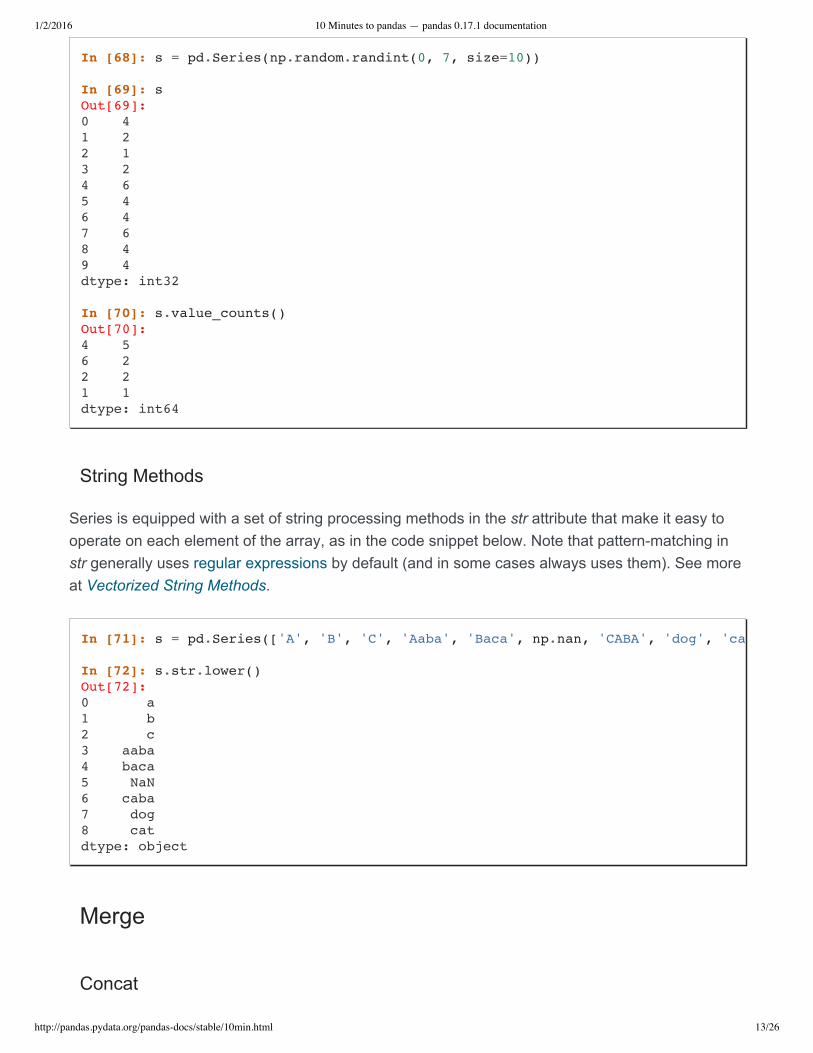
In [68]: s = pd.Series(np.random.randint(0, 7, size=10))

In [69]: s Out[69]: 0 4 1 2 2 1 3 2 4 6 5 4 6 4 7 6 8 4 9 4 dtype: int32

In [70]: s.value_counts() Out[70]: 4 5 6 2 2 2 1 1 dtype: int64

String Methods

Series is equipped with a set of string processing methods in the str attribute that make it easy tooperate on each element of the array, as in the code snippet below. Note that pattern­matching instr generally uses regular expressions by default (and in some cases always uses them). See moreat Vectorized String Methods.

Merge

Concat

In [71]: s = pd.Series(['A', 'B', 'C', 'Aaba', 'Baca', np.nan, 'CABA', 'dog', 'cat'

In [72]: s.str.lower() Out[72]: 0 a 1 b 2 c 3 aaba 4 baca 5 NaN 6 caba 7 dog 8 cat dtype: object

1/2/2016 10 Minutes to pandas — pandas 0.17.1 documentation

http://pandas.pydata.org/pandas-docs/stable/10min.html 14/26

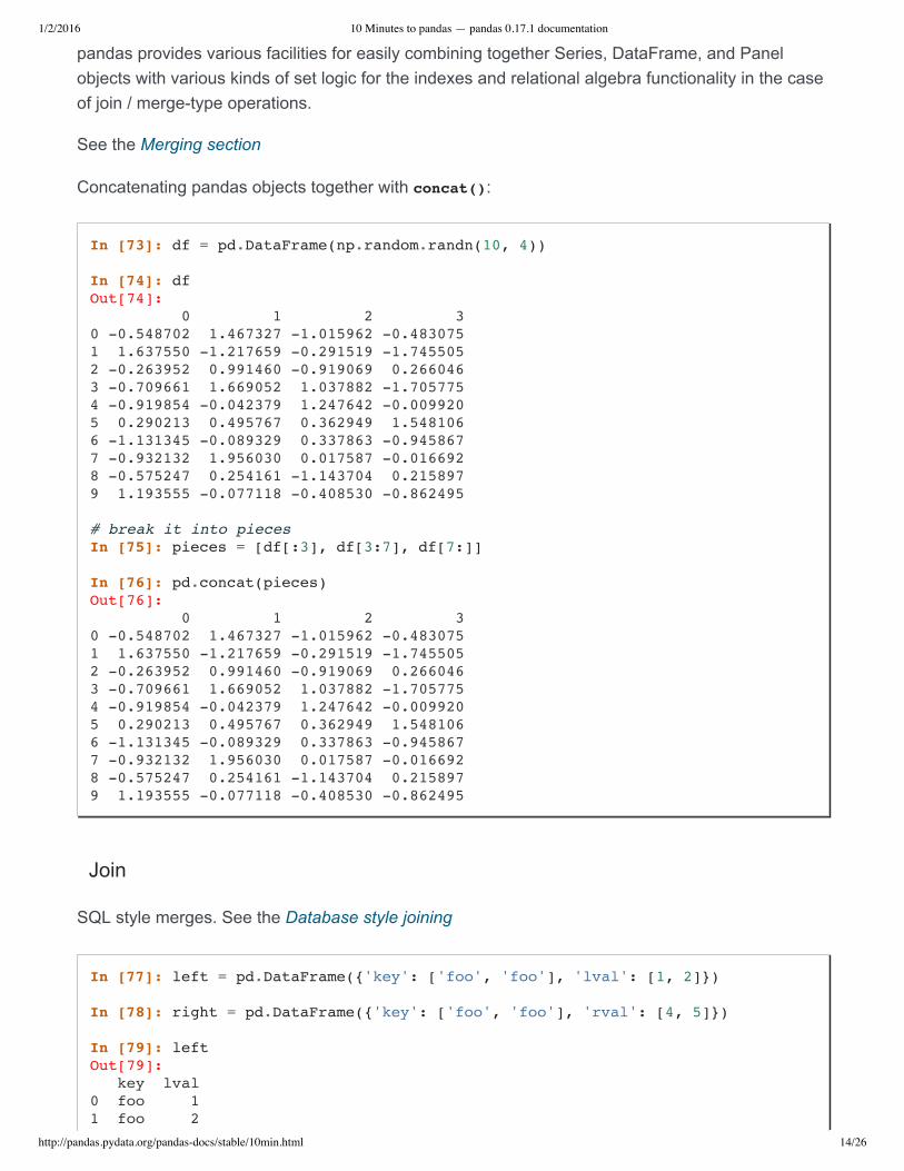
pandas provides various facilities for easily combining together Series, DataFrame, and Panelobjects with various kinds of set logic for the indexes and relational algebra functionality in the caseof join / merge­type operations.

See the Merging section

Concatenating pandas objects together with concat():

In [73]: df = pd.DataFrame(np.random.randn(10, 4))

In [74]: df Out[74]: 0 1 2 3 0 -0.548702 1.467327 -1.015962 -0.483075 1 1.637550 -1.217659 -0.291519 -1.745505 2 -0.263952 0.991460 -0.919069 0.266046 3 -0.709661 1.669052 1.037882 -1.705775 4 -0.919854 -0.042379 1.247642 -0.009920 5 0.290213 0.495767 0.362949 1.548106 6 -1.131345 -0.089329 0.337863 -0.945867 7 -0.932132 1.956030 0.017587 -0.016692 8 -0.575247 0.254161 -1.143704 0.215897 9 1.193555 -0.077118 -0.408530 -0.862495

# break it into pieces In [75]: pieces = [df[:3], df[3:7], df[7:]]

In [76]: pd.concat(pieces) Out[76]: 0 1 2 3 0 -0.548702 1.467327 -1.015962 -0.483075 1 1.637550 -1.217659 -0.291519 -1.745505 2 -0.263952 0.991460 -0.919069 0.266046 3 -0.709661 1.669052 1.037882 -1.705775 4 -0.919854 -0.042379 1.247642 -0.009920 5 0.290213 0.495767 0.362949 1.548106 6 -1.131345 -0.089329 0.337863 -0.945867 7 -0.932132 1.956030 0.017587 -0.016692 8 -0.575247 0.254161 -1.143704 0.215897 9 1.193555 -0.077118 -0.408530 -0.862495

Join

SQL style merges. See the Database style joining

In [77]: left = pd.DataFrame('key': ['foo', 'foo'], 'lval': [1, 2])

In [78]: right = pd.DataFrame('key': ['foo', 'foo'], 'rval': [4, 5])

In [79]: left Out[79]: key lval 0 foo 1 1 foo 2

1/2/2016 10 Minutes to pandas — pandas 0.17.1 documentation

http://pandas.pydata.org/pandas-docs/stable/10min.html 15/26

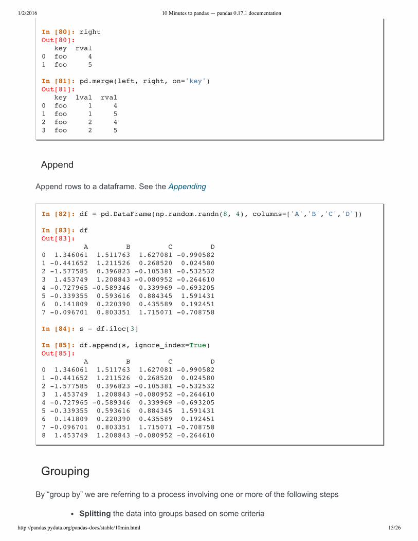
Append

Append rows to a dataframe. See the Appending

Grouping

By “group by” we are referring to a process involving one or more of the following steps

Splitting the data into groups based on some criteria

In [80]: right Out[80]: key rval 0 foo 4 1 foo 5

In [81]: pd.merge(left, right, on='key') Out[81]: key lval rval 0 foo 1 4 1 foo 1 5 2 foo 2 4 3 foo 2 5

In [82]: df = pd.DataFrame(np.random.randn(8, 4), columns=['A','B','C','D'])

In [83]: df Out[83]: A B C D 0 1.346061 1.511763 1.627081 -0.990582 1 -0.441652 1.211526 0.268520 0.024580 2 -1.577585 0.396823 -0.105381 -0.532532 3 1.453749 1.208843 -0.080952 -0.264610 4 -0.727965 -0.589346 0.339969 -0.693205 5 -0.339355 0.593616 0.884345 1.591431 6 0.141809 0.220390 0.435589 0.192451 7 -0.096701 0.803351 1.715071 -0.708758

In [84]: s = df.iloc[3]

In [85]: df.append(s, ignore_index=True) Out[85]: A B C D 0 1.346061 1.511763 1.627081 -0.990582 1 -0.441652 1.211526 0.268520 0.024580 2 -1.577585 0.396823 -0.105381 -0.532532 3 1.453749 1.208843 -0.080952 -0.264610 4 -0.727965 -0.589346 0.339969 -0.693205 5 -0.339355 0.593616 0.884345 1.591431 6 0.141809 0.220390 0.435589 0.192451 7 -0.096701 0.803351 1.715071 -0.708758 8 1.453749 1.208843 -0.080952 -0.264610

1/2/2016 10 Minutes to pandas — pandas 0.17.1 documentation

http://pandas.pydata.org/pandas-docs/stable/10min.html 16/26

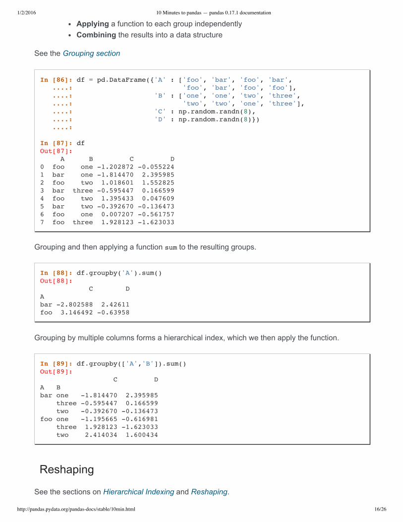
Applying a function to each group independentlyCombining the results into a data structure

See the Grouping section

Grouping and then applying a function sum to the resulting groups.

In [88]: df.groupby('A').sum() Out[88]: C D A bar -2.802588 2.42611 foo 3.146492 -0.63958

Grouping by multiple columns forms a hierarchical index, which we then apply the function.

In [89]: df.groupby(['A','B']).sum() Out[89]: C D A B bar one -1.814470 2.395985 three -0.595447 0.166599 two -0.392670 -0.136473 foo one -1.195665 -0.616981 three 1.928123 -1.623033 two 2.414034 1.600434

Reshaping

See the sections on Hierarchical Indexing and Reshaping.

In [86]: df = pd.DataFrame('A' : ['foo', 'bar', 'foo', 'bar', ....: 'foo', 'bar', 'foo', 'foo'], ....: 'B' : ['one', 'one', 'two', 'three', ....: 'two', 'two', 'one', 'three'], ....: 'C' : np.random.randn(8), ....: 'D' : np.random.randn(8)) ....:

In [87]: df Out[87]: A B C D 0 foo one -1.202872 -0.055224 1 bar one -1.814470 2.395985 2 foo two 1.018601 1.552825 3 bar three -0.595447 0.166599 4 foo two 1.395433 0.047609 5 bar two -0.392670 -0.136473 6 foo one 0.007207 -0.561757 7 foo three 1.928123 -1.623033

1/2/2016 10 Minutes to pandas — pandas 0.17.1 documentation

http://pandas.pydata.org/pandas-docs/stable/10min.html 17/26

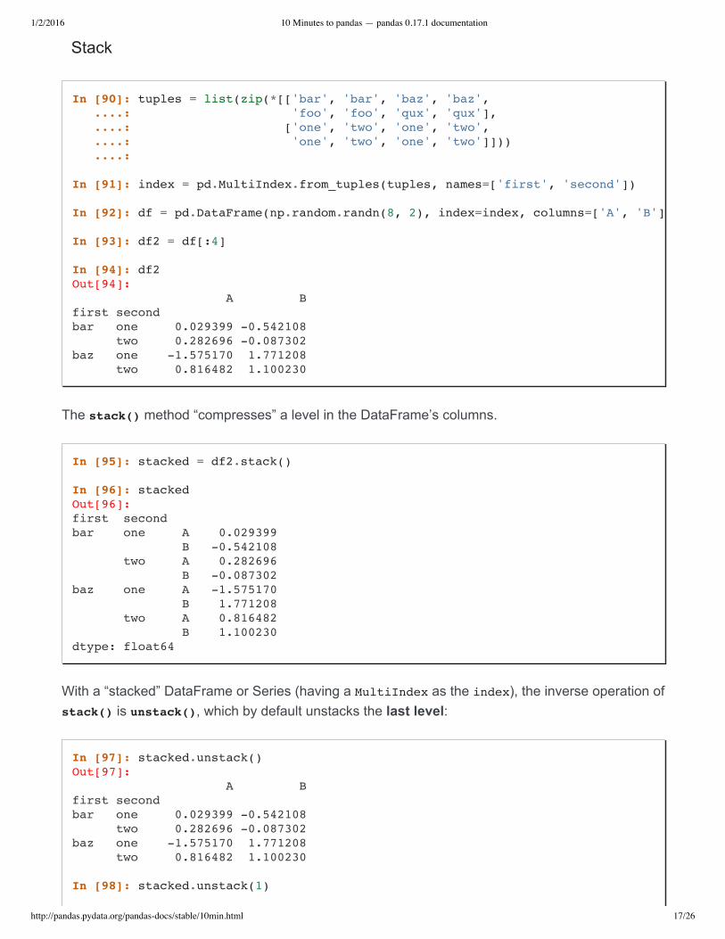
Stack

The stack() method “compresses” a level in the DataFrame’s columns.

In [95]: stacked = df2.stack()

In [96]: stacked Out[96]: first second bar one A 0.029399 B -0.542108 two A 0.282696 B -0.087302 baz one A -1.575170 B 1.771208 two A 0.816482 B 1.100230 dtype: float64

With a “stacked” DataFrame or Series (having a MultiIndex as the index), the inverse operation ofstack() is unstack(), which by default unstacks the last level:

In [97]: stacked.unstack() Out[97]: A B first second bar one 0.029399 -0.542108 two 0.282696 -0.087302 baz one -1.575170 1.771208 two 0.816482 1.100230

In [98]: stacked.unstack(1)

In [90]: tuples = list(zip(*[['bar', 'bar', 'baz', 'baz', ....: 'foo', 'foo', 'qux', 'qux'], ....: ['one', 'two', 'one', 'two', ....: 'one', 'two', 'one', 'two']])) ....:

In [91]: index = pd.MultiIndex.from_tuples(tuples, names=['first', 'second'])

In [92]: df = pd.DataFrame(np.random.randn(8, 2), index=index, columns=['A', 'B'])

In [93]: df2 = df[:4]

In [94]: df2 Out[94]: A B first second bar one 0.029399 -0.542108 two 0.282696 -0.087302 baz one -1.575170 1.771208 two 0.816482 1.100230

1/2/2016 10 Minutes to pandas — pandas 0.17.1 documentation

http://pandas.pydata.org/pandas-docs/stable/10min.html 18/26

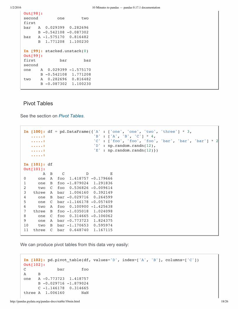
Out[98]: second one two first bar A 0.029399 0.282696 B -0.542108 -0.087302 baz A -1.575170 0.816482 B 1.771208 1.100230

In [99]: stacked.unstack(0) Out[99]: first bar baz second one A 0.029399 -1.575170 B -0.542108 1.771208 two A 0.282696 0.816482 B -0.087302 1.100230

Pivot Tables

See the section on Pivot Tables.

We can produce pivot tables from this data very easily:

In [100]: df = pd.DataFrame('A' : ['one', 'one', 'two', 'three'] * 3, .....: 'B' : ['A', 'B', 'C'] * 4, .....: 'C' : ['foo', 'foo', 'foo', 'bar', 'bar', 'bar'] * 2 .....: 'D' : np.random.randn(12), .....: 'E' : np.random.randn(12)) .....:

In [101]: df Out[101]: A B C D E 0 one A foo 1.418757 -0.179666 1 one B foo -1.879024 1.291836 2 two C foo 0.536826 -0.009614 3 three A bar 1.006160 0.392149 4 one B bar -0.029716 0.264599 5 one C bar -1.146178 -0.057409 6 two A foo 0.100900 -1.425638 7 three B foo -1.035018 1.024098 8 one C foo 0.314665 -0.106062 9 one A bar -0.773723 1.824375 10 two B bar -1.170653 0.595974 11 three C bar 0.648740 1.167115

In [102]: pd.pivot_table(df, values='D', index=['A', 'B'], columns=['C']) Out[102]: C bar foo A B one A -0.773723 1.418757 B -0.029716 -1.879024 C -1.146178 0.314665 three A 1.006160 NaN

1/2/2016 10 Minutes to pandas — pandas 0.17.1 documentation

http://pandas.pydata.org/pandas-docs/stable/10min.html 19/26

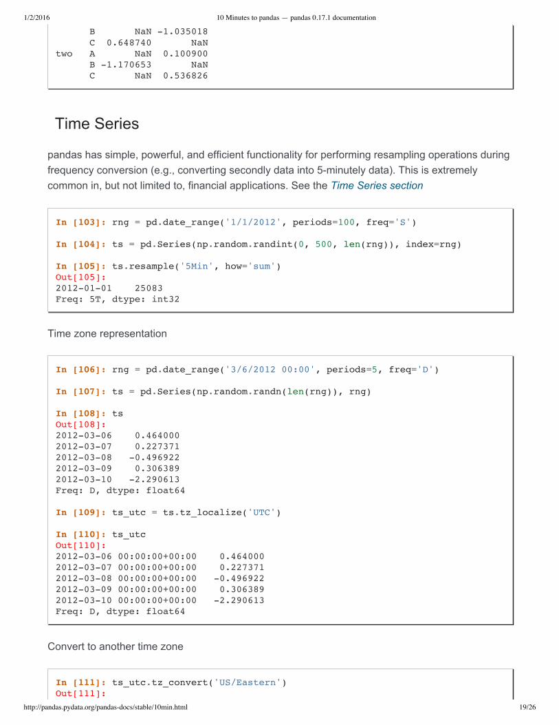
Time Series

pandas has simple, powerful, and efficient functionality for performing resampling operations duringfrequency conversion (e.g., converting secondly data into 5­minutely data). This is extremelycommon in, but not limited to, financial applications. See the Time Series section

Time zone representation

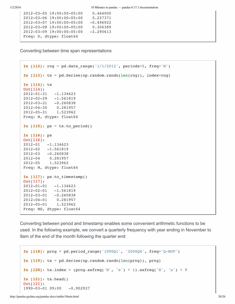
Convert to another time zone

In [111]: ts_utc.tz_convert('US/Eastern') Out[111]:

B NaN -1.035018 C 0.648740 NaN two A NaN 0.100900 B -1.170653 NaN C NaN 0.536826

In [103]: rng = pd.date_range('1/1/2012', periods=100, freq='S')

In [104]: ts = pd.Series(np.random.randint(0, 500, len(rng)), index=rng)

In [105]: ts.resample('5Min', how='sum') Out[105]: 2012-01-01 25083 Freq: 5T, dtype: int32

In [106]: rng = pd.date_range('3/6/2012 00:00', periods=5, freq='D')

In [107]: ts = pd.Series(np.random.randn(len(rng)), rng)

In [108]: ts Out[108]: 2012-03-06 0.464000 2012-03-07 0.227371 2012-03-08 -0.496922 2012-03-09 0.306389 2012-03-10 -2.290613 Freq: D, dtype: float64

In [109]: ts_utc = ts.tz_localize('UTC')

In [110]: ts_utc Out[110]: 2012-03-06 00:00:00+00:00 0.464000 2012-03-07 00:00:00+00:00 0.227371 2012-03-08 00:00:00+00:00 -0.496922 2012-03-09 00:00:00+00:00 0.306389 2012-03-10 00:00:00+00:00 -2.290613 Freq: D, dtype: float64

1/2/2016 10 Minutes to pandas — pandas 0.17.1 documentation

http://pandas.pydata.org/pandas-docs/stable/10min.html 20/26

2012-03-05 19:00:00-05:00 0.464000 2012-03-06 19:00:00-05:00 0.227371 2012-03-07 19:00:00-05:00 -0.496922 2012-03-08 19:00:00-05:00 0.306389 2012-03-09 19:00:00-05:00 -2.290613 Freq: D, dtype: float64

Converting between time span representations

Converting between period and timestamp enables some convenient arithmetic functions to beused. In the following example, we convert a quarterly frequency with year ending in November to9am of the end of the month following the quarter end:

In [112]: rng = pd.date_range('1/1/2012', periods=5, freq='M')

In [113]: ts = pd.Series(np.random.randn(len(rng)), index=rng)

In [114]: ts Out[114]: 2012-01-31 -1.134623 2012-02-29 -1.561819 2012-03-31 -0.260838 2012-04-30 0.281957 2012-05-31 1.523962 Freq: M, dtype: float64

In [115]: ps = ts.to_period()

In [116]: ps Out[116]: 2012-01 -1.134623 2012-02 -1.561819 2012-03 -0.260838 2012-04 0.281957 2012-05 1.523962 Freq: M, dtype: float64

In [117]: ps.to_timestamp() Out[117]: 2012-01-01 -1.134623 2012-02-01 -1.561819 2012-03-01 -0.260838 2012-04-01 0.281957 2012-05-01 1.523962 Freq: MS, dtype: float64

In [118]: prng = pd.period_range('1990Q1', '2000Q4', freq='Q-NOV')

In [119]: ts = pd.Series(np.random.randn(len(prng)), prng)

In [120]: ts.index = (prng.asfreq('M', 'e') + 1).asfreq('H', 's') + 9

In [121]: ts.head() Out[121]: 1990-03-01 09:00 -0.902937

1/2/2016 10 Minutes to pandas — pandas 0.17.1 documentation

http://pandas.pydata.org/pandas-docs/stable/10min.html 21/26

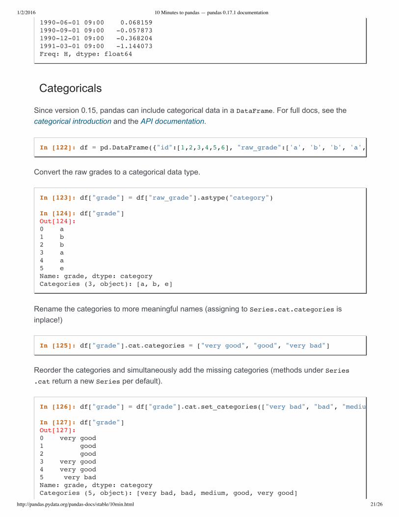
Categoricals

Since version 0.15, pandas can include categorical data in a DataFrame. For full docs, see thecategorical introduction and the API documentation.

Convert the raw grades to a categorical data type.

In [123]: df["grade"] = df["raw_grade"].astype("category")

In [124]: df["grade"] Out[124]: 0 a 1 b 2 b 3 a 4 a 5 e Name: grade, dtype: category Categories (3, object): [a, b, e]

Rename the categories to more meaningful names (assigning to Series.cat.categories isinplace!)

Reorder the categories and simultaneously add the missing categories (methods under Series.cat return a new Series per default).

1990-06-01 09:00 0.068159 1990-09-01 09:00 -0.057873 1990-12-01 09:00 -0.368204 1991-03-01 09:00 -1.144073 Freq: H, dtype: float64

In [122]: df = pd.DataFrame("id":[1,2,3,4,5,6], "raw_grade":['a', 'b', 'b', 'a',

In [125]: df["grade"].cat.categories = ["very good", "good", "very bad"]

In [126]: df["grade"] = df["grade"].cat.set_categories(["very bad", "bad", "medium"

In [127]: df["grade"] Out[127]: 0 very good 1 good 2 good 3 very good 4 very good 5 very bad Name: grade, dtype: category Categories (5, object): [very bad, bad, medium, good, very good]

1/2/2016 10 Minutes to pandas — pandas 0.17.1 documentation

http://pandas.pydata.org/pandas-docs/stable/10min.html 22/26

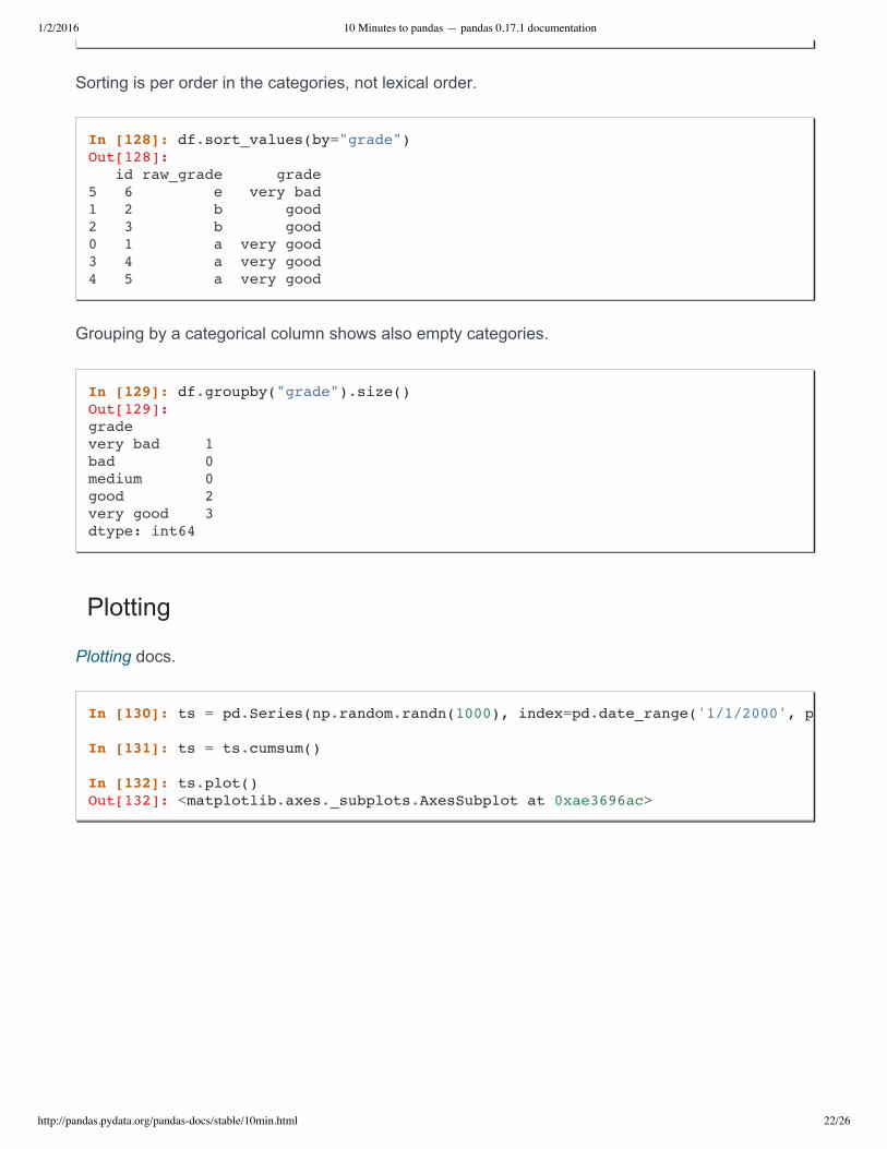
Sorting is per order in the categories, not lexical order.

In [128]: df.sort_values(by="grade") Out[128]: id raw_grade grade 5 6 e very bad 1 2 b good 2 3 b good 0 1 a very good 3 4 a very good 4 5 a very good

Grouping by a categorical column shows also empty categories.

In [129]: df.groupby("grade").size() Out[129]: grade very bad 1 bad 0 medium 0 good 2 very good 3 dtype: int64

Plotting

Plotting docs.

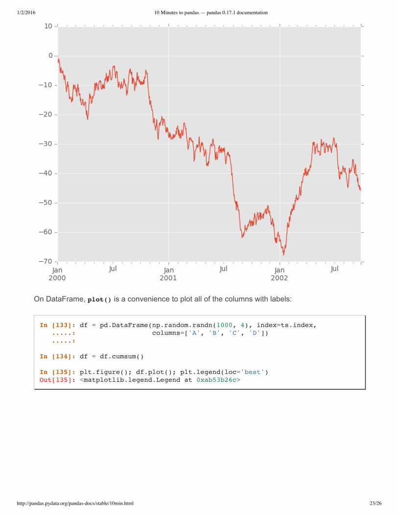
In [130]: ts = pd.Series(np.random.randn(1000), index=pd.date_range('1/1/2000', periods

In [131]: ts = ts.cumsum()

In [132]: ts.plot() Out[132]: <matplotlib.axes._subplots.AxesSubplot at 0xae3696ac>

1/2/2016 10 Minutes to pandas — pandas 0.17.1 documentation

http://pandas.pydata.org/pandas-docs/stable/10min.html 23/26

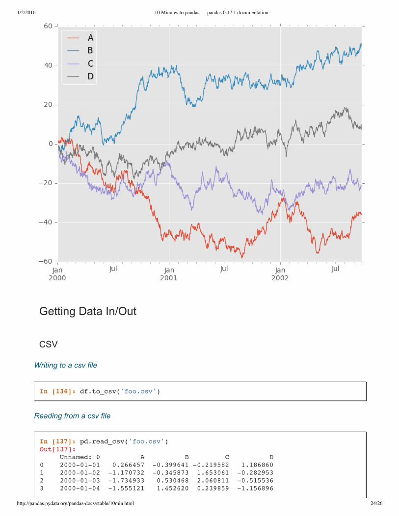
On DataFrame, plot() is a convenience to plot all of the columns with labels:

In [133]: df = pd.DataFrame(np.random.randn(1000, 4), index=ts.index, .....: columns=['A', 'B', 'C', 'D']) .....:

In [134]: df = df.cumsum()

In [135]: plt.figure(); df.plot(); plt.legend(loc='best') Out[135]: <matplotlib.legend.Legend at 0xab53b26c>

1/2/2016 10 Minutes to pandas — pandas 0.17.1 documentation

http://pandas.pydata.org/pandas-docs/stable/10min.html 24/26

Getting Data In/Out

CSV

Writing to a csv file

In [136]: df.to_csv('foo.csv')

Reading from a csv file

In [137]: pd.read_csv('foo.csv') Out[137]: Unnamed: 0 A B C D 0 2000-01-01 0.266457 -0.399641 -0.219582 1.186860 1 2000-01-02 -1.170732 -0.345873 1.653061 -0.282953 2 2000-01-03 -1.734933 0.530468 2.060811 -0.515536 3 2000-01-04 -1.555121 1.452620 0.239859 -1.156896

1/2/2016 10 Minutes to pandas — pandas 0.17.1 documentation

http://pandas.pydata.org/pandas-docs/stable/10min.html 25/26

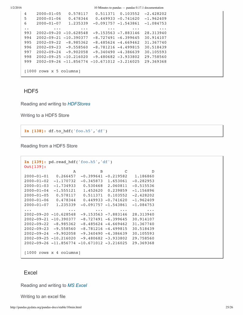
4 2000-01-05 0.578117 0.511371 0.103552 -2.428202 5 2000-01-06 0.478344 0.449933 -0.741620 -1.962409 6 2000-01-07 1.235339 -0.091757 -1.543861 -1.084753 .. ... ... ... ... ... 993 2002-09-20 -10.628548 -9.153563 -7.883146 28.313940 994 2002-09-21 -10.390377 -8.727491 -6.399645 30.914107 995 2002-09-22 -8.985362 -8.485624 -4.669462 31.367740 996 2002-09-23 -9.558560 -8.781216 -4.499815 30.518439 997 2002-09-24 -9.902058 -9.340490 -4.386639 30.105593 998 2002-09-25 -10.216020 -9.480682 -3.933802 29.758560 999 2002-09-26 -11.856774 -10.671012 -3.216025 29.369368

[1000 rows x 5 columns]

HDF5

Reading and writing to HDFStores

Writing to a HDF5 Store

In [138]: df.to_hdf('foo.h5','df')

Reading from a HDF5 Store

In [139]: pd.read_hdf('foo.h5','df') Out[139]: A B C D2000-01-01 0.266457 -0.399641 -0.219582 1.1868602000-01-02 -1.170732 -0.345873 1.653061 -0.2829532000-01-03 -1.734933 0.530468 2.060811 -0.5155362000-01-04 -1.555121 1.452620 0.239859 -1.1568962000-01-05 0.578117 0.511371 0.103552 -2.4282022000-01-06 0.478344 0.449933 -0.741620 -1.9624092000-01-07 1.235339 -0.091757 -1.543861 -1.084753... ... ... ... ...2002-09-20 -10.628548 -9.153563 -7.883146 28.3139402002-09-21 -10.390377 -8.727491 -6.399645 30.9141072002-09-22 -8.985362 -8.485624 -4.669462 31.3677402002-09-23 -9.558560 -8.781216 -4.499815 30.5184392002-09-24 -9.902058 -9.340490 -4.386639 30.1055932002-09-25 -10.216020 -9.480682 -3.933802 29.7585602002-09-26 -11.856774 -10.671012 -3.216025 29.369368

[1000 rows x 4 columns]

Excel

Reading and writing to MS Excel

Writing to an excel file

1/2/2016 10 Minutes to pandas — pandas 0.17.1 documentation

http://pandas.pydata.org/pandas-docs/stable/10min.html 26/26

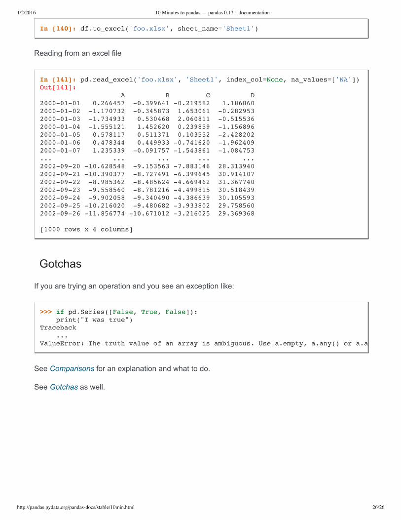
In [140]: df.to_excel('foo.xlsx', sheet_name='Sheet1')

Reading from an excel file

Gotchas

If you are trying an operation and you see an exception like:

See Comparisons for an explanation and what to do.

See Gotchas as well.

In [141]: pd.read_excel('foo.xlsx', 'Sheet1', index_col=None, na_values=['NA']) Out[141]: A B C D2000-01-01 0.266457 -0.399641 -0.219582 1.1868602000-01-02 -1.170732 -0.345873 1.653061 -0.2829532000-01-03 -1.734933 0.530468 2.060811 -0.5155362000-01-04 -1.555121 1.452620 0.239859 -1.1568962000-01-05 0.578117 0.511371 0.103552 -2.4282022000-01-06 0.478344 0.449933 -0.741620 -1.9624092000-01-07 1.235339 -0.091757 -1.543861 -1.084753... ... ... ... ...2002-09-20 -10.628548 -9.153563 -7.883146 28.3139402002-09-21 -10.390377 -8.727491 -6.399645 30.9141072002-09-22 -8.985362 -8.485624 -4.669462 31.3677402002-09-23 -9.558560 -8.781216 -4.499815 30.5184392002-09-24 -9.902058 -9.340490 -4.386639 30.1055932002-09-25 -10.216020 -9.480682 -3.933802 29.7585602002-09-26 -11.856774 -10.671012 -3.216025 29.369368

[1000 rows x 4 columns]

>>> if pd.Series([False, True, False]): print("I was true") Traceback ... ValueError: The truth value of an array is ambiguous. Use a.empty, a.any() or a.all().