GW100: Benchmarking G0W0 for Molecular SystemsMichiel J. van Setten,*,1,2 Fabio Caruso,4,5 Sahar Sharifzadeh,6,16 Xinguo Ren,4,9 Matthias Scheffler,4

Fang Liu,10 Johannes Lischner,7,11 Lin Lin,8 Jack R. Deslippe,12 Steven G. Louie,7,11 Chao Yang,8

Florian Weigend,2,3 Jeffrey B. Neaton,6,11,13 Ferdinand Evers,14 and Patrick Rinke4,15

1Nanoscopic Physics, Institute of Condensed Matter and Nanosciences, Universite Catholique de Louvain, Louvain-la-Neuve, 1348,Belgium2Institute of Nanotechnology and 3Institute of Physical Chemistry, Karlsruhe Institute of Technology Campus North, Karlsruhe,76344 Germany4Fritz-Haber-Institut der Max-Planck-Gesellschaft, Berlin, 14195, Germany5Department of Materials, University of Oxford, Oxford, OX1 3PH, United Kingdom6Molecular Foundry, 7Materials Sciences Division, and 8Computational Research Division, Lawrence Berkeley National Laboratory,Berkeley, California 94720, United States9Key Laboratory of Quantum Information, University of Science and Technology of China, Hefei, 230026, China10School of Applied Mathematics, Central University of Finance and Economics, Beijing, China11Department of Physics, University of California, Berkeley, California 94720, United States12National Energy Research Scientific Computing Center, Berkeley, California 94720, United States13Kavli Energy NanoSciences Institute at Berkeley, Berkeley, California 94720 United States14Institute of Theoretical Physics, University of Regensburg, Regensburg, 93040, Germany15COMP/Department of Applied Physics, Aalto University School of Science, Aalto 00076, Finland16Department of Electrical and Computer Engineering, Department of Physics, Division of Materials Science and Engineering, BostonUniversity, Boston, Massachusetts 02215, United States

*S Supporting Information

ABSTRACT: We present the GW100 set. GW100 is a benchmark set of theionization potentials and electron affinities of 100 molecules computed withthe GW method using three independent GW codes and different GWmethodologies. The quasi-particle energies of the highest-occupiedmolecular orbitals (HOMO) and lowest-unoccupied molecular orbitals(LUMO) are calculated for the GW100 set at the G0W0@PBE level usingthe software packages TURBOMOLE, FHI-aims, and BerkeleyGW. The useof these three codes allows for a quantitative comparison of the type of basisset (plane wave or local orbital) and handling of unoccupied states, thetreatment of core and valence electrons (all electron or pseudopotentials),the treatment of the frequency dependence of the self-energy (full frequency or more approximate plasmon-pole models), andthe algorithm for solving the quasi-particle equation. Primary results include reference values for future benchmarks, bestpractices for convergence within a particular approach, and average error bars for the most common approximations.

1. INTRODUCTION

Computational spectroscopy is developing into a complemen-tary approach to experimental spectroscopy. It facilitates theinterpretation of experimental spectra and can predict proper-ties of hitherto unexplored materials. In computationalspectroscopy, as in any other theoretical discipline, the firststep is the definition of the physical model. In theoreticalphysics and chemistry, this model is governed by a set ofequations. Computational sciences solve these equationsnumerically, and the solutions should of course be independentfrom the computational settings. However, in reality this is notalways the case. In practice, the equations are often

complicated, and the numerical techniques introduce many,often interdependent, computational parameters. A thoroughvalidation of these parameters can be very time-consuming.To validate computational approaches, theoretical bench-

marks are essential. In quantum chemistry, benchmark sets arewell-established (e.g., G2/97,1−3 GMTKN30,4 ISO34,5,6 S667).In solid state physics, a validation benchmark set for elementarysolids has only recently been published for ground stateproperties calculated in density-functional theory (DFT).8

Received: May 16, 2015

Article

pubs.acs.org/JCTC

© XXXX American Chemical Society A DOI: 10.1021/acs.jctc.5b00453J. Chem. Theory Comput. XXXX, XXX, XXX−XXX

According to refs 8 and 9, several DFT codes differ by asurprising amount even for the computationally efficientsemilocal Perdew−Burke−Ernzerhof (PBE) functional.10The physical model we address in this article describes

charged electronic excitations, and we apply it here tomolecules. We focus on Hedin’s GW approximation11 whereG is the single particle Green’s function and W the screenedCoulomb interaction. For solids, GW has become the methodof choice for the calculation of quasi-particle spectra asmeasured in direct and inverse photoemission.12−14 Recently,the GW approach has also increasingly been applied tomolecules and nanostructures.15−53

In its simplest form (G0W0), the GW approach is applied as acorrection to the electronic spectrum of a noninteractingreference Hamiltonian, such as Kohn−Sham DFT or Hartree−Fock11−14 (in the following denoted @reference). However,despite G0W0’s more than 50 year history and, starting 30 yearsago, its practical implementation within an electronic structureframework,54−56 results from different codes and approxima-tions have rarely been directly compared. In this article, weprovide a thorough assessment of G0W0, with a particularstarting point, for gas-phase molecules using three differentcodes, validating different computational implementations andelucidating best practices for convergence parameters, such asbasis sets, treatment of the unoccupied subspace, anddiscretization meshes.In this work, we make the first step and establish a consistent

set of benchmarks of ionization energies and electron affinitiesof 100 molecules−the GW100 set. We present converged G0W0calculations based on the Perdew−Burke−Ernzerhof (PBE)10generalized gradient approximation to DFT. Our G0W0@PBEresults for these molecules can serve as a reference for futureG0W0 implementations and calculations. We apply threedifferent G0W0 codes in this work: TURBOMOLE,49,57 FHI-aims,40,58 and BerkeleyGW.59 The three codes differ in theirchoice of basis set (atom centered orbitals in TURBOMOLEand FHI-aims and plane waves in BerkeleyGW) and in theirimplementation. The validation process was crucial to removeconceptual and numerical inconsistencies from our implemen-tations and to test the influence of all computational settings. Inthe end, all three codes agree on average within 0.2 eV forionization energies and electron affinities. TURBOMOLE andFHI-aims are all-electron codes and use the same basis sets inthis work. (The calculations perfomed in this work are allexplicitly nonrelitivistic to exclude the effects of differentrelativistic approaches. The QZVP basis sets for fifth rowelements used in this work are also fully all-electron and do notcontain an effective core potential.) They agree to ∼1 meV.BerkeleyGW, employing a real-axis full-frequency method andpseudopotentials, leads to results that differ from TURBO-MOLE and FHI-aims by 200 meV on average. We consider thisdifference in residual discrepancy as acceptable for the timebeing because FHI-aims and TURBOMOLE use the exact same(local-orbital) basis set, and BerkeleyGW uses a plane wavebasis set with pseudopotentials. The plane wave basis set makesBerkeleyGW also applicable to extended systems. Whether ornot there is another dominating source remains to beinvestigated.In the GW100 set, we also supply experimental ionization

energies and electron affinities, where available. These areintended for future reference. Care has to be taken in thecomparison to experimental values, because experimental datatends to carry uncertainties that are intrinsic to the measuring

process or reflect external influences (e.g., defects or disorder)and other environmental parameters (e.g., temperature). Theseeffects, and intrinsic effects such as the zero-point motion, arenot included in our current theoretical approach. An assess-ment of the GW method as such is beyond the scope of thiswork and would require an extensive study of the starting pointdependence of G0W0.

14,39,42,43,47,51,60,61 Indeed, the depend-ence on the starting point is a well-known problem ofperturbative GW calculations for molecules as well, which canbe solved only through fully self-consistent GW calcula-tions.29,39,62,63 The starting-point dependence for local andsemilocal DFT functional starting points are usually small (<0.1eV49). Considering the whole range of starting-points fromsemilocal DFT to Hartree−Fock, the starting-point depend-ence can easily exceed 1.0 eV.29,49,64 In this work, we do notinvestigate the starting point dependence and only compareresults obtained using PBE as a starting point.Before moving on to discuss the actual results of the GW

methods described above, we comment on the differences incomputational cost between the G0W0 method and otherapproaches that may be employed in the evaluation of thequasi-particle excitations of molecules. G0W0 calculations aresignificantly more demanding than local or semilocal DFTcalculations and comparable in cost to advanced DFTcalculations in, for example, the random-phase approxima-tion.65−68 The high numerical cost of G0W0 calculations mostlystems from the computation of the polarizability and of thescreened Coulomb interaction. The precise computationalbottlenecks that limit the applicability of the G0W0 method tolarge systems depends on the type of basis function that isadopted in the calculation. In plane wave-codes, the mainbottleneck arises from the necessity to include a large vacuumregion to avoid spurious interactions between the fictitiousperiodic replicas of the system. As a consequence, a largenumber of reciprocal-lattice vectors are required to numericallyconverge the calculations, which makes the computation of thepolarizability very demanding. In localized-basis code, such asFHI-aims and TURBOMOLE, on the other hand, the mostdemanding computational operation is the evaluation andstorage of the Coulomb integrals, which are typically handledwithin the framework of the resolution-of-the-identity.Numerical implementations of the G0W0 approach typically

scale as N( )3 or N( )4 with N being the number of basisfunctions. The scaling with system size is the same. Despitetheir high numerical cost, G0W0 calculations remain consid-erably cheaper than wave function-based approaches, such ascoupled-cluster singles-doubles (CCSD), CCSD with triples(CCSDT), or configuration interaction (CI). In these methods,the main computational bottlenecks arise from the complexansatz adopted for the many-body wave function, whichrequires the explicit inclusion of the excited Slater determi-nants. Correspondingly, the scaling of computational costrelative to system size is typically N( )6 for CCSD, N( )8 forCCSDT, and exponential for full CI.The remainder of the article is structured as follows: We start

by describing the test set that will be used in this paper insection 2. In section 3, we present the G0W0 approaches used inthis work and explain their similarities and differences. Insection 4, the ionization energies and electron affinities of theGW100 are presented. In section 5, we discuss the differentways to treat the analytic structure of W in our three G0W0approaches. The main conclusions are summarized in section 6.

Journal of Chemical Theory and Computation Article

DOI: 10.1021/acs.jctc.5b00453J. Chem. Theory Comput. XXXX, XXX, XXX−XXX

B

2. THE GW100 SET

The 100 molecules in the GW100 set include different elementsand thereby cover a considerable range of ionization potentials(from ∼4 eV for Rb2 to ∼25 eV for He). The selectedmolecules exhibit a spectrum of typical chemical bondingsituations. For instance, for carbon, we include a variety ofcovalent bonds, such as C2H6, C2H4, C2H2, C6H6, CO, CO2,and C4. Special interest is devoted to bonds of metal atoms byincluding Cu2 and Ag2, Li2, K2, Na2, and Rb2 as well as smallmetallic clusters Na4 and Na6. In contrast, alkaline metal halidesare prototypes for ionic bonds with LiF being an extreme andKBr a more moderate case. The alkaline earth metalcompounds MgF2 and MgO are also ionic, the former with avanishing and the latter with a large dipole moment. Includingseries of homologous like N2-P2-As2, F2-Cl2-Br2-I2, or CF4,CCl4, CBr4, or CI4 facilitates the identification of trends withina group of elements. These trends can then be correlated withcertain physical or chemical properties, such as the decreasingionic bond character in the last example. Furthermore, we havealso included several simple organic molecules, like alcohols,aldehydes, and nitrogenous bases, as well as the most typicaltest cases often appearing in benchmark sets such as water andcarbon mono- and dioxide.We have considered using a standard test set, for example,

the G2 set. This was not done for the following reasons: First,some of the GW codes are restricted to closed-shell systems,and the G2 set contains many open-shell systems, for example,the alkaline atoms. Second, it is restricted to compounds of thefirst two periods, excluding the elements Li, Be, Na, Mg, and Aland thus covers neither bonds between metal atoms norpronounced ionic bonds. Third, it contains only smallmolecules in which the degree of delocalization is rathersmall. In our work, we observe that none of the ninecompounds that show a discrepancy between GW resulting inlarger than 1 eV in the IP at GW-level is contained in the G2set. The respective systems turn out to be strongly ionicalkaline (earth) hydrides, fluorides, chlorides, bromides, andoxides as well as C4 and O3. The worst case that is also presentin the G2 set is FH with a maximal discrepancy of 0.8 eV. Wewould thus not expect any other G2 molecule to show a largerdeviation.The molecular geometries used in this work are mainly taken

from experimental data. For some molecules, the final structurewas obtained by optimizing a known morphology using DFT inthe PBE approximation for the exchange-correlation functionalusing the def2-QZVP basis set. All molecular geometries areincluded in the Supporting Information.

3. COMPUTATIONAL METHODOLOGY

The objective of this work is to establish a set of converged andvalidated G0W0 results for molecules that will serve as abenchmark for future work. Specifically, we calculate the G0W0self-energy11

∫ωπ

ω ω ω ωΣ ′ = ′ ′ + ′ ′ ′σ σ

−∞

+∞G Wr r r r r r( , , )

2d ( , , ) ( , , )0 0

(1)

where G0σ denotes the one-particle causal Green’s function for

spin channel σ = ↑,↓ and W0 is the screened Coulombinteraction in the random-phase approximation (RPA). Tradi-tionally, one splits the self-energy into energy dependentcorrelation and energy independent exchange terms as

ω ωΣ = Σ + Σσ σ σ( ) ( )x c (2)

G0σ is given in terms of the single-particle wave functions

ψnσKS(r) and eigenvalues ϵnσ

KS of a reference Kohn−Sham DFTcalculation.69

∑ωψ ψ

ω η′ =

′− ϵ − ϵ − ϵ

σ σ σ

σ σ

*

G r rr r

( , , )( ) ( )

sgn( )n

n n

n n0

KS KS

KSF

KS(3)

where ϵF is the Fermi level (chemical potential) and η a positiveinfinitesimal. W0 follows from the noninteracting responsefunction χ0 that in a real-space representation assumes thefollowing form

∫χ ωπ

ω ω ω ω′ = − ′ ′ + ′ ′ ′σ σ

−∞

+∞G Gr r r r r r( , , )

2d ( , , ) ( , , )0 0 0

(4)

∑ ∑ψ ψ ψ ψ

ω η=

− ′ ′

− ϵ + ϵ +σ

σ σ σ σ

σ σ

* *f f r r r r( ) ( ) ( ) ( ) ( )

n m

n m n m m n

m n,

KS KS KS KS

KS KS(5)

where the second line is the sum-over states representation ofAdler and Wiser,70,71 and fm and f n are the occupation factors ofstates m and n, respectively. Given the noninteracting responsefunction χ0, W0 is expanded in powers of χ0

χ χ χ χ= + + + ··· = +W v v v v v v v v v0 0 0 0 (6)

where we have omitted the space and frequency variables forsimplicity. The last equal sign in eq 6 introduces the reducibleresponse function χ = χ0[1 − vχ0]

−1.Given the G0W0 self-energy, the quasi-particle (QP) energies

εnQP are computed by solving the diagonal QP equation in thebasis of the single-particle states |nσ⟩, i.e.

ε σ ε σ= ϵ + ⟨ |Σ − | ⟩σ σσ

σn v n( )n n nQP KS QP

xc (7)

In the above equation, vxc denotes the exchange-correlationpotential of the preceding DFT calculation. Since we willrestrict ourselves to closed shell molecules for the remainder ofthe paper, we drop the spin index σ.In our comparative study, we use a DFT-PBE starting point.

Once we have decided on this reference Hamiltonian, G0 isuniquely defined. As a result, Σ in the G0W0 approximation isalso uniquely defined and all G0W0 implementations should, inprinciple, produce the same G0W0@PBE results. However,G0W0 implementations can differ in several aspects, that inpractice can lead to deviations. The most critical aspects arelisted as follows:

(a). The Choice of Basis Set. In this work, we will compareGW results obtained with both local orbital (LO) and planewave (PW) basis sets. In a local basis set, the size of theHamiltonian is usually significantly smaller than in plane waves.For example, for ethene with the LO basis used here,approximately 350 functions were used; the analogous planewave calculation used a factor of 225 more functions. However,for an LO basis, there is no unique recipe to systematicallyincrease the basis set to approach the complete basis set limit.Conversely, a plane wave basis set is conceptually easier toconverge: one main parameter, the kinetic energy cutoff, needsto be increased until convergence is achieved. However, planewaves require periodic boundary conditions, and moleculestherefore have to be placed in a supercell, which is a large,periodically repeated box that is filled with vacuum. Althoughthe size of the supercell usually convergences quickly for localand semi-local DFT functionals, the screened Coulomb

Journal of Chemical Theory and Computation Article

DOI: 10.1021/acs.jctc.5b00453J. Chem. Theory Comput. XXXX, XXX, XXX−XXX

C

interaction W0 in G0W0 can be long-ranged. A brute forcesupercell convergence is therefore computationally impracti-cal.72 Instead, the Coulomb interaction is truncated,73,74 whichintroduces, in principle, an additional convergence parameter.In BerkeleyGW, this truncation is automatically based onsupercell size. To compute ionization energies and electronaffinities, we correct for the shift in vacuum level that is presentdue to periodic boundary conditions. Taking the molecule atthe center of the supercell, the vacuum correction is calculatedas the electrostatic potential at the supercell edges.In plane wave G0W0 calculations, additional energy cutoffs

are often introduced that reduce the number of unoccupiedstates included in the empty state summations of the Green’sfunction (eq 3) and the noninteracting response function (eq5).75−77 These energy cutoffs can reduce the computationalcost, albeit at the expense of new convergence parameters.78,79

Conversely, the use of a small number of basis functions in localorbital calculations can limit the number and the accuracy ofempty states above the vacuum level. If in this situation asystematic extrapolation to the basis set limit is not feasible, thiscan lead to limitations in the accuracy of the response functiongiven by eq 5 and G0 and W0 and, therefore, the self-energyitself.G0W0 has also been implemented in other basis sets, such as

projector augmented waves (PAW), see refs 75, 80, and 81 forexamples, and linear augmented plane waves (LAPW), see refs82−85 for examples, and linearized muffin tin orbitals(LMTO), see ref 86 for an example. These implementationshave not been included in the present test.(b). The Treatment of Core Electrons and Valence

Electrons in the Core Regions. In the FHI-aims andTURBOMOLE calculations in this work, we included allelectrons explicitly at each step of the calculation. However, atthe moment, a pure plane wave basis set requirespseudopotentials that remove the rapid oscillations of theelectronic wave functions near the nuclei and hence drasticallyreduce the required energy cutoff. In a pseudopotentialapproach, the electrons are divided into core and valenceelectrons. The core electrons are frozen in their atomic groundstate and are used to generate a smooth potential for thevalence electrons.87−92 On the DFT level, pseudopotentials aretypically derived from single-atom DFT calculations performedwith the same functional as used later.However, interactions between core and valence electrons

that depend on the environment in a polyatomic systemundermine transferability and lead to deviations betweenpseudopotentials and all-electron calculations. The use ofpseudopotentials can lead to errors in GW calculations becauseof the neglect of core polarization effects,14,93 deviations in thepseudo and all-electron wave functions near the nucleus,94,95

and core−valence interactions.94,95 To shed more light on thequantitative role of core electrons and pseudopotentials, wedirectly compare all-electron, frozen core, and pseudopotentialG0W0 calculations in this work.DFT-PBE pseudopotentials are used in our planewave G0W0

calculations. All valence electrons of the same principalquantum number are treated on the G0W0 level, whereas thedescription of the core electrons and the core−valenceinteraction remains on the DFT level.(c). Treatment of the Frequency Dependence. All

quantities in G0W0 depend explicitly on a frequency (or time)argument (see section 3). Different G0W0 implementationsdiffer in their treatment of this frequency dependence. Because

the poles in G0 and all subsequent quantities lie close to the realfrequency axis, all quantities in G0W0 exhibit a pronounced finestructure on the real frequency axis, whose resolution requiresfine frequency grids and a large number of frequency points.Different strategies are employed to avoid the computationalbottleneck of dense frequency grids. In this work, we willcompare several different ways: the fully analytic treatment inTURBOMOLE (TM-RI) and (TM-noRI),49 an integration onthe imaginary axis with subsequent analytic continuation to thereal axis as implemented in FHI-aims (AIMS-2P) and (AIMS-P16),40,58 and the BerkeleyGW implementation of the fullfrequency treatment on the real axis (BGW-FF)96 and of ageneralized plasmon pole model (BGW-GPP).55 Techniquesemploying contour deformation and approaches to circumventthe sum over empty states have also been reported in theliterature,97−101 but they are not considered in this work.

(d). Solution of the QP Equation. The final step in G0W0is the calculation of the QP -energies by solving eq 7. Atechnical aspect that we draw particular attention to is theoccurrence of multiple solutions in the QP equation.102−104

Because not all GW codes search for all solutions, differentG0W0 implementations may give different answers for multiple-solution cases even though the underlying self-energies may bevery similar.In summary, the impact of these differing approaches (a−d)

can affect the QP energies in a significant way, which has onlyin part been quantified by previous studies.40,45,49,94,95 Apartfrom code validation, a second main goal of our work is aquantitative comparison of different methods. This goal will beachieved by comparing the G0W0 results (i.e., the QP energies)obtained from three different G0W0 implementations: TUR-BOMOLE, FHI-aims, and BerkeleyGW.In the following sections, we describe the conceptual and

technical differences that distinguish the TURBOMOLE, FHI-aims, and BerkeleyGW G0W0 implementations. A more generaldescription of the GW method and its application to moleculesin particular can be found in various reviews12−14,49,105,106 andis not the topic of this paper. We will also provide detailedconvergence studies of the relevant computational parameters.

3.1. The Frequency Dependence of the G0W0 Self-Energy. A pronounced difference between different G0W0implementations is the treatment of the frequency dependenceof the self-energy in eq 1 and of intermediate quantities. In thiswork, we will compare an analytic treatment of the polestructure facilitated by the spectral representation of theresponse function with a plasmon-pole model and a numericalreal as well as imaginary frequency treatment. In the next foursections, we describe the technical aspects of these approaches.The implications on the results of these different approacheswill be discussed in the Results and Discussion sections.

3.1.1. Implementation of the Fully Analytic (FA) SpectralRepresentation in TURBOMOLE. The RPA response function(eqs 5 and 6) is calculated explicitly in its spectralrepresentation. Because the Green’s function G0 has Nocc +Nunocc poles, the screened interactionW0 exhibits 2 × NoccNunoccpoles. As the exact pole positions of W0 are inherited from G0and therefore known, we can evaluate the energy integral for Σ(eq 1) analytically. This gives for Σ 2 × (Nocc + Nunocc)NoccNunocc poles. In the rest of this section, we summarize themost important technical details following ref 49, where wehere focus on the nonmagnetic case ψ = ψ↑ = ψ↓.The implementation of G0W0 in TURBOMOLE is based on

the spectral representation of the reducible response function.

Journal of Chemical Theory and Computation Article

DOI: 10.1021/acs.jctc.5b00453J. Chem. Theory Comput. XXXX, XXX, XXX−XXX

D

∑χ ω ρ ρω η ω η

′ = ′+ − Ω

−− + Ω

⎛⎝⎜

⎞⎠⎟r r r r( , , ) ( ) ( )

1 1

mm m

m m

(8)

The pole positions, Ωm, are the (charge neutral) excitationenergies, and ρm(r) denotes transition densities. The ρm areexpanded in a basis of orbital products,

∑ρ ψ ψ= +X Yr r r( ) ( ) ( ) ( )mi a

m m i a i a,

,KS KS

(9)

where i,j,.. label occupied states, and a,b,.. label empty states.The vectors |Xm,Ym⟩ are solutions of the eigenvalue problem

Λ − Ω Δ | ⟩ =X Y( ) , 0m m m (10)

under the orthonormality constraint

δ⟨ |Δ| ⟩ =′ ′ ′X Y X Y, ,m m m m m m, (11)

The operators

Λ = Δ =−

⎛⎝⎜

⎞⎠⎟

⎛⎝⎜

⎞⎠⎟

A BB A

,1 00 1 (12)

contain the orbital rotation Hessians

δ δ+ = ϵ − ϵ + ⟨ | ⟩ij ab(A B) ( ) 2iajb a i ij ab (13)

δ δ− = ϵ − ϵ(A B) ( )iajb a i ij ab (14)

with ∫ ψ ψ ψ ψ⟨ | ⟩ = ′ ′ ′| − ′|r r r r r rij ab d d ( ) ( ) ( ) ( )i j a br rKS KS 1 KS KS .

From the reducible response function, the screenedCoulomb interaction W can be directly constructed bycontracting with the Coulomb interaction v

ω χ ω= + · ·W v v v( ) ( ) (15)

The self-energy can finally be obtained directly by perform-ing the energy integral analytically because in this formalism theenergy structure of both G and W is known. Performing theintegral leads to a closed expression for the matrix elements ofthe self-energy. The real part of the diagonal matrix elements ofΣ includes the exchange contribution

∑⟨ |Σ | ⟩ = − |n n ni in( )i

x

(16)

while for the correlation contribution, we have

∑ ∑

∑

ρη

ρη

ℜ ⟨ |Σ ϵ | ⟩ = | | |ϵ − ϵ + Ω

ϵ − ϵ + Ω +

+ | | |ϵ − ϵ − Ω

ϵ − ϵ − Ω +

⎡⎣⎢⎢

⎤⎦⎥⎥

n n in

an

( ( ) )12

( )( )

( )( )

nm i

mn i m

n i m

am

n a m

n a m

c 22 2

22 2

(17)

where, as before, m runs over all density excitations, and η is aninfinitesimal.

3.1.2. BerkeleyGW Implementation of the Full Frequency(FF) Integration along the Real Frequency Axis. The FF-BerkeleyGW approach evaluates the frequency-dependent self-energy numerically along the real frequency axis. Similar to theTURBOMOLE implementation, G0, W0, and Σ retain the fullpole structure. However, unlike in TURBOMOLE, the polestructure is represented on the frequency grid.In FF-BerkeleyGW the frequency dependent self-energy is

∫

∫

∑

∑

∑

ω ψ ψ

πψ ψ

ω ω ωω ω η

πψ ψ

ω ω ωω ω η

Σ ′ = − * ′ ′

− * ′

′ ′ ′ − ′ ′− ϵ + ′ −

− * ′

′ ′ ′ − ′ ′− ϵ − ′ +

=

=

∞

= +

+

∞

v

i

W Wi

i

W Wi

r r r r r r

r r

r r r r

r r

r r r r

( , , ) ( ) ( ) ( , )

12

( ) ( )

d( , , ) ( , , )

12

( ) ( )

d( , , ) ( , , )

j

N

j j

j

N

j j

r a

j

a N

N N

a a

a

a

r

1

KS KS

1

KS KS

0 KS

1

KS KS

0 KS

occ

occ

occ

occ unocc

(18)

where Wr/a are the retarded (r) and advanced (a) screenedCoulomb matrix, which can be expressed as

∫ω ω′ ≡ ϵ ″ ″ ′ ″−W vr r r r r r r( , , ) [ ( , , )] ( , ) dr a r a/ / 1(19)

where the retarded/advanced dielectric function ϵr/a has theform

∫ω δ χ ωϵ ′ = ′ − ″ ″ ′ ″vr r r r r r r r r( , , ) ( , ) ( , ) ( , , ) dr a r a/0

/

and the retarded/advanced reducible polarizability is defined as

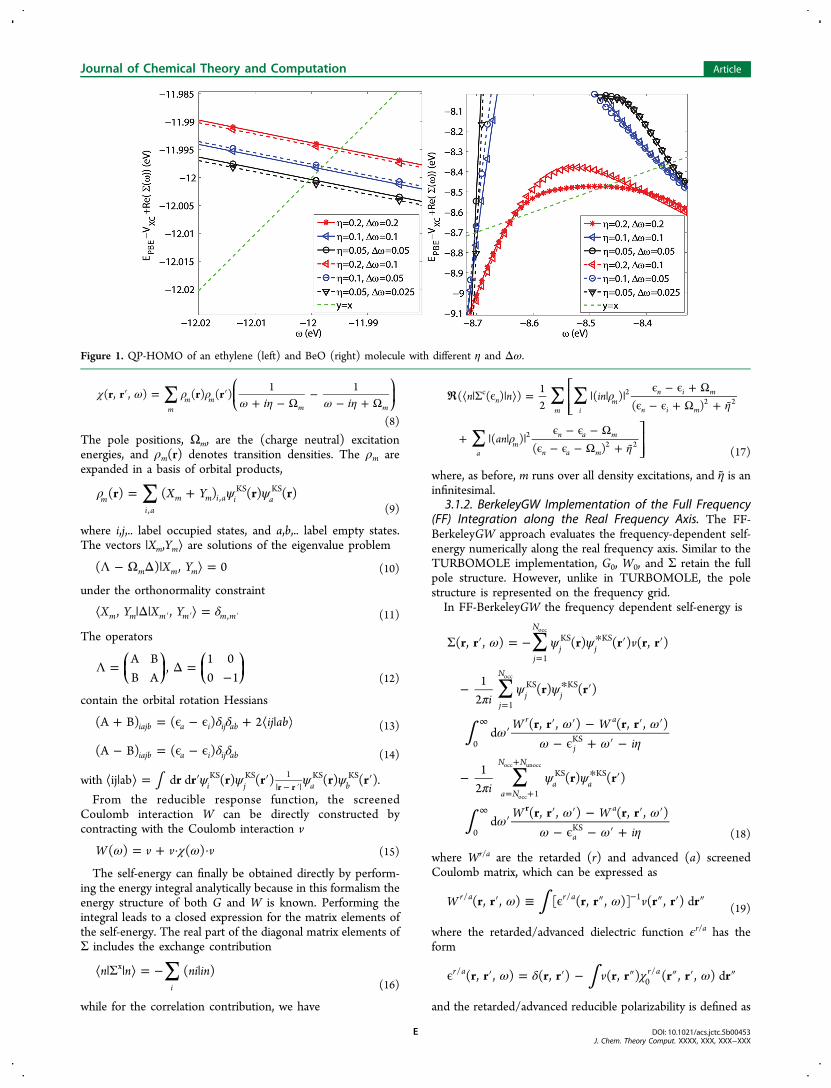
Figure 1. QP-HOMO of an ethylene (left) and BeO (right) molecule with different η and Δω.

Journal of Chemical Theory and Computation Article

DOI: 10.1021/acs.jctc.5b00453J. Chem. Theory Comput. XXXX, XXX, XXX−XXX

E

∑ ∑χ ω ψ ψ ψ ψ

ω η ω η

′ = * * ′ ′

×− Δϵ ±

−+ Δϵ ±

= = +

+

⎛⎝⎜⎜

⎞⎠⎟⎟i i

r r r r r r( , , )12

( ) ( ) ( ) ( )

1 1

r a

i

N

j N

N N

i j i j

i j i j

0/

1 1

KS KS KS KS

,KS

,KS

occ

occ

occ unocc

(20)

where Δϵi,j = ϵj − ϵi ≥ 0.The integral in eq 18 is evaluated numerically on the interval

[0,ωhighcut ], beyond which the integrand is negligibly small. We

further reduce computational cost by dividing the interval[0,ωhigh

cut ] into two intervals: [0,ωlowcut ] and [ωlow

cut ,ωhighcut ] treated

with two different integration schemes. The low frequencycutoff ωlow

cut is chosen to ensure that all poles of the numerator inthe integrand lie below ωlow

cut ; therefore, the integrand decayssmoothly beyond this point. A uniform fine frequency step Δωis used on [0,ωlow

cut ], whereas a smaller number of quadraturepoints can be used to perform a standard numerical integrationof eq 18 within the interval [ωlow

cut ,ωhighcut ]. Because the integrand

contains a number of singularities in the interval [0,ωlowcut ], we

use the special integration scheme of ref 107 to perform thenumerical integration accurately on this interval.For all 18 of the molecules studied with FF-BGW, we use η =

0.2 eV and Δω = 0.2 eV. The left panel of Figure 1 shows atypical example (ethylene molecule) of the convergence withthe dependence of the quasi-particle energy on the parametersη and Δω for predicted QP-HOMO energy. Because our aimhere is to test the convergence behavior for η and Δω, we useda low Eϵ

cut of 5.0 Ry (68 eV). (In principle, we use eV as theenergy unit; however, in cases where the input parameters of aspecific code are supplied in another unit, we also provide thequantity in this unit.) Figure 1 shows that for a given η, Δω = ηis sufficient for an accuracy of 0.01 eV, and that η = 0.2 eV issufficient. The right panel of Figure 1 shows an example for amolecule with a large slope of the self-energy. Here, aconvergence within 0.2 eV is reached.In a plane wave basis, the number of basis functions is much

larger than in the localized basis set used in TURBOMOLE andFHI-aims. Therefore, intermediate quantities, such as thedielectric function and the self-energy, require larger matrices.To keep the calculation tractable, we only computed thedielectric function for a reduced set of plane waves with planewave cutoff energy Eϵ

cut. In addition, the number of unoccupiedstates that enter the Green’s function and the self-energy iscontrolled by the energy of the highest unoccupied state, Emax.Because Eϵ

cut and Emax are interdependent,37 careful convergence

studies are required. Here, we converged these parameterswithin GPP-GW as will be described below. We converged thedielectric function by increasing both Emax and Eϵ

cut until thescreened exchange component of the self-energy changed byless than 0.2 eV and extrapolated the Coulomb-hole term of theself-energy by means of the static completion method.108

Within this approach, a term is added to the Coulomb-holecomponent of Σ, which corrects for the truncation of thenumber of unoccupied states.108

In Table 1, the values of the parameters introduced in thissection are listed for 18 molecules studied with FF-BGW. Forall FF-BGW calculations, values of η = 0.2 eV, Δω = 0.2 eV,and Eϵ

cut = 24 Ry (326 eV) have been used.3.1.3. FHI-aims Implementation of the Imaginary

Frequency Treatment Including Analytic Continuation(AC). In imaginary frequency implementations, G0, W0, and Σretain their full pole structure but on the imaginary frequencyaxis. This representation requires significantly fewer frequency

points due to the smooth behavior of all quantities on theimaginary frequency axis. The self-energy is then analyticallycontinued to the real frequency axis. The “quality” of the self-energy on the real-frequency axis depends on the type ofanalytic continuation.FHI-aims provides two different analytic continuation

models: (i) a “two-pole fit”109 and (ii) a Pade approximation(see ref 110). In the “two-pole fit”, each matrix element of theself-energy is fitted to the following expression on the imaginaryaxis

∑ωω

Σ ≃+=

ia

i b( )ij

n

n

n1

2

(21)

where the dependence of a and b on i and j has been omittedfor simplicity. In the Pade approximation, Σij is given by

ωω ω

ω ωΣ ≃

+ + +

+ + +−

−

ia a i a i

b i b i( )

( ) ... ( )

1 ( ) ... ( )ijN

N

NN

0 1 ( 1)/2( 1)/2

1 /2/2

(22)

where N is the total number of parameters employed in thePade expansion. The ionization energies and electron affinitiesin Tables 2 and 5 have been calculated using N = 16 (which isequivalent to a sum of 8 poles). Σ on the real-frequency axis isthen obtained by replacing iω with ω in eqs 21 or 22, and theG0W0 quasi-particle energies are obtained by solving eq 7.

3.1.4. Generalized Plasmon Pole (GPP) in the BerkeleyGWImplementation. Within our GPP implementation,59 theexpression for the self-energy, Σ, is written as the sum of twoterms, termed the screened-exchange (SX) and Coulomb-hole(CH). Here,

∑ω ψ ψω ω

Σ = * × Ω − Φ− ϵ − =

iv( ) ( )

(1 tan )( )j

N

j jj

SX1

KS KS2

2 2

v

(23)

and

Table 1. Computational Parameters for 18 MoleculesComputed within FF-BGWa

molecule Ewfncut (Ry (eV)) Nv

b Ncc ωlow

cut (eV)

acetylene 80 (1088) 5 1659 115.0methane 90 (1225) 4 1253 115.0vinyl bromide 80 (1088) 9 2644 120.0ethylene 80 (1088) 6 832 115.0ethane 80 (1088) 7 1939 115.0acetaldehyde 100 (1361) 9 1909 120.0N2 120 (1633) 5 905 120.0H2O 110 (1497) 4 770 120.0BeO 110 (1497) 4 1183 115.0MgO 110 (1497) 4 2033 115.0LiH 60 (816) 1 2504 100.0CO2 110 (1497) 8 911 125.0COS 110 (1497) 8 1724 120.0F2 90 (1225) 7 531 125.0MgF2 90 (1225) 8 1223 120.0C2H3F 90 (1225) 9 1566 125.0H2O2 110 (1497) 7 925 125.0N2H4 110 (1497) 7 1404 120.0

aColumns 2, 3, and 5 are fixed at the converged value from the BGW-GPP calculation. bNumber of valence bands cNumber of conductionbands

Journal of Chemical Theory and Computation Article

DOI: 10.1021/acs.jctc.5b00453J. Chem. Theory Comput. XXXX, XXX, XXX−XXX

F

Table 2. Ionization Potentials (the Negative of the QP-HOMO Energies) of the GW100 Set Calculated with G0W0@PBE usingTURBOMOLE, FHI-aims, and BerkeleyGWa

name formula AIMS-2P AIMS-P16 BGW-GPP BGW-FF TM-RI TM-noRI EXTRA exp.

1 helium He 23.44 23.48 24.10 23.24 23.48 23.49(0.03) 24.592 neon Ne 20.45 20.38 21.35 20.26 20.38 20.33(0.01) 21.563 argon Ar 15.07 15.13 15.94 15.04 15.13 15.28(0.03) 15.764 krypton Kr 13.49 13.57 14.00 13.55 13.57 13.89(0.16) 14.005 xenon Xe 12.03 12.02 12.08 11.97 12.02 12.136 hydrogen123 H2 15.81 15.81 16.23 15.68 15.82 15.85(0.09) 15.437 lithium dimer123 Li2 5.14 4.99 5.43 4.98 4.99 5.05(0.02) 4.738 sodium dimer123 Na2 5.04 4.83 5.03 4.82 4.85 4.88(0.03) 4.899 sodium tetramer124 Na4 4.16 4.10 4.34 4.10 4.12 4.14(0.03) 4.2710 sodium hexamer124 Na6 4.17 4.24 4.47 4.23 4.24 4.34(0.06) 4.1211 potassium dimer123 K2 4.20 3.98 4.02 3.97 3.98 4.08(0.04) 4.0612 rubidium dimer125 Rb2 4.01 3.80 3.92 3.79 3.79 3.9013 nitrogen123 N2 14.81 14.89 15.43 14.72 14.85 14.89 15.05(0.04) 15.58*14 phosphorus dimer123 P2 10.04 10.21 10.66 10.18 10.21 10.38(0.04) 10.62*15 arsenic dimer123 As2 9.28 9.47 9.67 9.47 9.47 9.67(0.10) 10.00*16 fluorine123 F2 14.92 14.96 15.59 14.73 14.85 14.96 15.10(0.04) 15.70*17 chlorine123 Cl2 10.98 11.10 11.85 11.03 11.10 11.31(0.05) 11.4918 bromine123 Br2 10.11 10.22 10.64 10.20 10.22 10.56(0.18) 10.5119 iodine123 I2 9.15 9.28 9.58 9.23 9.36*20 methane123 CH4 13.90 13.93 14.28 13.80 13.86 13.93 14.00(0.06) 14.35*21 ethane123 C2H6 12.30 12.37 12.63 12.22 12.30 12.37 12.46(0.06) 12.20*22 propane126 C3H8 11.74 11.79 12.05 11.73 11.80 11.89(0.06) 11.51*23 butane123 C4H10 11.42 11.49 11.73 11.42 11.59(0.05) 11.09*24 ethylene123 C2H4 10.17 10.33 10.68 10.30 10.30 10.33 10.40(0.03) 10.68*25 ethyn123 C2H2 10.93 11.02 11.35 10.97 11.00 11.02 11.09(0.01) 11.49*26 tetracarbon127 C4 10.73 10.78 11.49 10.75 10.91(0.03) 12.5427 cyclopropane123 C3H6 10.47 10.56 10.93 10.52 10.56 10.65(0.04) 10.54*28 benzene123 C6H6 8.92 8.99 9.21 8.97 9.10(0.01) 9.23*29 cyclooctatetraene128 C8H8 7.97 8.06 8.47 8.04 8.18(0.02) 8.43*30 cyclopentadiene123 C5H6 8.24 8.35 8.77 8.33 8.45(0.02) 8.53*31 vinyl fluoride123 C2H3F 10.08 10.20 10.80 10.14 10.16 10.20 10.32(0.02) 10.63*32 vinyl chloride123 C2H3Cl 9.68 9.76 10.32 9.73 9.76 9.89(0.02) 10.20*33 vinyl bromide123 C2H3Br 8.81 8.99 9.42 8.97 9.14(0.01) 9.90*34 vinyl iodide123 C2H3I 8.95 9.04 9.48 9.01 9.35*35 tetrafluoromethane123 CF4 15.29 15.37 15.96 15.27 15.37 15.60(0.06) 16.20*36 tetrachloromethane123 CCl4 10.89 10.98 11.77 10.92 11.21(0.06) 11.69*37 tetrabromomethane123 CBr4 9.81 9.90 10.40 9.89 10.22(0.16) 10.54*38 tetraiodomethane123 CI4 8.78 8.82 9.23 8.71 9.10*39 silane123 SiH4 12.21 12.31 12.77 12.23 12.31 12.40(0.06) 12.82*40 germane123 GeH4 11.92 12.02 12.28 11.95 12.02 12.11(0.04) 12.46*41 disilane123 Si2H6 10.21 10.31 10.80 10.25 10.30 10.41(0.06) 10.53*42 pentasilane127 Si5H12 8.82 8.94 9.45 8.89 9.05(0.05) 9.36*43 lithium hydride123 LiH 7.09 6.54 7.85 6.67 6.51 6.55 6.58(0.04) 7.9044 potassium hydride123 KH 5.20 4.86 5.76 4.82 4.86 4.99(0.01) 8.0045 borane123 BH3 12.82 12.87 13.28 12.79 12.87 12.96(0.06) 12.0346 diborane123 B2H6 11.78 11.84 12.17 11.76 11.84 11.93(0.06) 11.90*47 ammonia123 NH3 10.29 10.32 10.93 10.27 10.32 10.39(0.05) 10.82*48 hydrazoic acid123 HN3 10.25 10.39 10.96 10.36 10.40 10.55(0.02) 10.72*49 phosphine123 PH3 10.18 10.27 10.79 10.22 10.27 10.35(0.05) 10.59*50 arsine123 AsH3 10.09 10.12 10.45 10.10 10.12 10.21(0.02) 10.58*51 hydrogen sulfide123 SH2 9.94 10.03 10.64 9.97 10.03 10.13(0.04) 10.50*52 hydrogen fluoride123 FH 15.26 15.30 16.24 15.20 15.30 15.37(0.01) 16.12*53 hydrogen chloride123 ClH 12.16 12.25 12.97 12.18 12.25 12.36(0.01) 12.7954 lithium fluoride123 LiF 10.38 9.95 11.84 9.89 9.95 10.27(0.03) 11.3055 magnesium fluoride123 F2Mg 12.72 12.32 13.73 12.44 12.26 12.32 12.50(0.06) 13.3056 titanium tetrafluoride123 TiF4 14.01 13.89 14.88 13.82 13.90 14.07(0.05)57 aluminum fluoride123 AlF3 14.28 14.25 15.11 14.17 14.25 14.48(0.06) 15.45*58 boron monofluoride123 BF 10.42 10.56 11.49 10.53 10.56 10.73(0.05) 11.0059 sulfur tetrafluoride129 SF4 11.99 12.12 12.79 12.04 12.12 12.38(0.07) 12.0060 potassium bromide123 BrK 7.71 7.30 7.99 7.30 7.31 7.57(0.13) 8.82*

Journal of Chemical Theory and Computation Article

DOI: 10.1021/acs.jctc.5b00453J. Chem. Theory Comput. XXXX, XXX, XXX−XXX

G

∑ω ψ ψω ω ω

Σ = * × Ω − Φ − ϵ − ″

″ ″″

iv( )

12

( )(1 tan )

( )nn n

nCH

KS KS2

(24)

where j runs over occupied states, n″ runs over both occupied

and unoccupied states, and Ω, ω, λ, and Φ are the effective bare

plasma frequency, GPP mode frequency, amplitude, and phase

of the renormalized Ω2, respectively, defined in reciprocal space

as

ω ρρ

Ω =+ + ′

| + |− ′

′ qq G q G

q GG G

0( )

( )( ) ( )( )GG

2p2

2(25)

ωλ

=| |

Φ′′

′q

qq

( )( )

cos ( )GG2 GG

GG (26)

λδ

| | =Ω− ϵ′

Φ ′

′ ′−

′eqq

q( )

( )( ; 0)

i qGG

( ) GG2

GG GG1

GG

(27)

Here, ρ is the electron charge density in reciprocal space, andωp

2= 4πρ(0)e2/m is the classical plasma frequency. Theconvolution of G0 and W0 is performed analytically. Finally,Σ contains the same number of poles as G0 in this setting.As mentioned above, GW calculations within any basis

require thorough convergence studies because the dielectricfunction and self-energy converge slowly with respect to the

Table 2. continued

name formula AIMS-2P AIMS-P16 BGW-GPP BGW-FF TM-RI TM-noRI EXTRA exp.

61 gallium monochloride123 GaCl 9.54 9.55 10.24 9.53 9.55 9.74(0.07) 10.07*62 sodium chloride123 NaCl 8.54 8.10 9.60 8.06 8.10 8.43(0.14) 9.80*63 magnesium chloride123 MgCl2 11.05 10.99 11.98 10.95 10.99 11.20(0.07) 11.80*64 aluminum iodide123 AlI3 9.28 9.32 9.67 9.30 9.66*65 boron nitride123 BN 11.19 11.03† 12.19 9.68 11.00 11.01 11.15(0.03)66 hydrogen cyanide123 NCH 13.13 13.21 13.87 13.19 13.21 13.32(0.01) 13.61*67 phosphorus mononitride123 PN 11.03 11.14 12.13 11.10 11.14 11.29(0.04) 11.8868 hydrazine123 H2NNH2 9.25 9.28 9.78 9.10 9.23 9.28 9.37(0.04) 8.98*69 formaldehyde123 H2CO 10.32 10.33 11.02 10.25 10.33 10.46(0.02) 10.89*70 methanol123 CH4O 10.50 10.56 11.14 10.49 10.56 10.67(0.05) 10.96*71 ethanol130 C2H6O 10.12 10.16 10.57 10.09 10.27(0.05) 10.64*72 acetaldehyde123 C2H4O 9.59 9.55 10.16 9.43 9.48 9.55 9.66(0.03) 10.24*73 ethoxy ethane131 C4H10O 9.30 9.32 9.70 9.27 9.42(0.05) 9.61*74 formic acid123 CH2O2 10.78 10.73 11.39 10.67 10.73 10.87(0.01) 11.50*75 hydrogen peroxide123 HOOH 10.92 10.99 11.58 10.82 10.90 10.99 11.10(0.01) 11.70*76 water123 H2O 11.92 11.97 12.75 11.68 11.89 11.97 12.05(0.03) 12.62*77 carbon dioxide123 CO2 13.04 13.25 13.81 13.17 13.18 13.25 13.46(0.06) 13.77*78 carbon disulfide123 CS2 9.62 9.75 10.37 9.70 9.75 9.95(0.05) 10.09*79 carbon oxide sulfide123 OCS 10.73 10.91 11.49 11.02 10.86 10.91 11.11(0.05) 11.19*80 carbon oxide selenide123 OCSe 10.08 10.20 10.55 10.18 10.43(0.09) 10.37*81 carbon monoxide123 CO 13.37 13.57 14.33 13.53 13.57 13.71(0.04) 14.01*82 ozone123 O3 11.91 11.39† 13.05 12.00 11.36 11.39 11.49(0.03) 12.73*83 sulfur dioxide123 SO2 11.74 11.82 12.55 11.76 11.82 12.06(0.06) 12.50*84 beryllium monoxide123 BeO 9.35 8.58† 10.66 9.68 8.60 8.62 8.60(0.01) 10.1085 magnesium monoxide123 MgO 7.03 6.68† 8.51 7.08 6.66 6.66 6.75(0.03) 8.7686 toluene123 C7H8 8.48 8.61 8.97 8.59 8.73(0.02) 8.82*87 ethylbenzene127 C8H10 8.44 8.55 8.92 8.54 8.66(0.02) 8.77*88 hexafluorobenzene126 C6F6 9.43 9.49 10.04 9.45 9.74(0.07) 10.20*89 phenol123 C6H5OH 8.28 8.37 8.72 8.34 8.51(0.01) 8.75*90 aniline123 C6H5NH2 7.61 7.64 7.98 7.62 7.78(0.02) 8.05*91 pyridine123 C5H5N 9.08 9.04 9.50 9.01 9.17(0.01) 9.51*92 guanine127 C5H5N5O 7.60 7.69 7.92 7.67 7.87(0.01) 8.24*93 adenine127 C5H5N5O 7.92 7.98 8.35 7.95 8.16(0.01) 8.48*94 cytosine127 C4H5N3O 8.25 8.29 8.77 8.26 8.44(0.01) 8.94*95 thymine127 C5H6N2O2 8.58 8.71 9.19 8.68 8.87(0.01) 9.20*96 uracil127 C4H4N2O2 9.37 9.22 9.94 9.17 9.38(0.01) 9.68*97 urea132 CH4N2O 9.38 9.32 9.94 9.27 9.46(0.02) 10.15*98 silver dimer133 Ag2 7.14 7.07 8.37 7.08 7.6699 copper dimer134 Cu2 7.54 7.55 8.33 7.52 7.53 7.78(0.06) 7.46100 copper cyanide123 NCCu 9.79 9.42† 10.80 9.41 9.56(0.04)

aThe first column denotes the molecule’s index. The AIMS-2P, AIMS-P16, TM-RI, and TM-noRI results have been calculated with a def2-QZVPbasis. Extrapolated AIMS-P16 results (see section 3.2) are shown in column EXTRA. The estimated errors for the extrapolated results (ERR),calculated as absolute difference between basis-set size and cardinal number extrapolation, are given in brackets. No extrapolated values are presentedfor molecules containing fifth row elements because SVP and TZVP all-electron basis sets are not available. The AIMS values marked with † arecalculated using a 128 parameter Pade fit. The experimental geometries are taken from the references listed behind each molecule. The experimentalionization energies, taken from the NIST database,122 are reported for comparison. Experimental values marked * correspond to vertical ionizationenergies.

Journal of Chemical Theory and Computation Article

DOI: 10.1021/acs.jctc.5b00453J. Chem. Theory Comput. XXXX, XXX, XXX−XXX

H

energy of the highest unoccupied state (Emax) included in thecalculation as well as the G-vector cutoff for the dielectricmatrix (Eϵ

cut). Moreover, these parameters are interdependent.37

We tested the convergence of the quasi-particle energies byvarying Emax such that the unoccupied states reached 30, 45, 90,120, and 150 eV above the vacuum level while simultaneouslyvarying Eϵ

cut from 82, 163, 327, and 408 to 544 eV. We note thatEmax defines the number of unoccupied states used to constructthe dielectric function and the self-energy, whereas Eϵ

cut affectsthe self-energy only through its effect on the dielectric function.Because of the computational cost of these convergence

studies, we systematically checked the convergence of thecalculated ionization energies and electron affinities of only 35randomly chosen molecules and applied consistent conver-gence parameters to all 100 molecules. An example of theconvergence of the ionization energy is shown for magnesiumoxide and ozone in Figure 2. We determined that, at Emax = 90eV and Eϵ

cut = 408 eV, the error was less than 0.2 eV for all butthe ozone molecule (see Figure 3) when compared to the

highest convergence criteria tested (Emax = 150 eV and Eϵcut =

544 eV). Therefore, this was set as the convergence criteria forall 100 molecules. When computationally feasible (for 10additional molecules), we checked that going beyond thisconvergence criteria did not alter predicted energies for theremaining molecules by more than 0.2 eV. The ozone moleculewas exceptionally difficult to converge and required a highernumber of unoccupied states. The reported value of ionizationenergy and electron affinity of ozone was Emax = 120 eV andEϵcut = 544 eV.In our pseudopotentials for transition metal atoms, semicore

d-states are explicitly treated as valence. Here, the density that isused to construct the plasma frequency does not include thesemicore, but inclusion of semicore electrons is necessary fordescribing the nodal structure of the valence wave function.111

Because the planewave cutoff is very high with the use ofsemicore states, we performed a limited convergence study forCu2 of the influence of dielectric function cutoffs and numberof bands. We estimate an error of ∼0.3 eV for the predictedionization energies and electron affinities of these transitionmetal-containing compounds.

3.2. Basis Sets. Types of Local Basis Sets. The G0W0 QPenergies in TURBOMOLE and FHI-aims are calculated usingthe TURBOMOLE def2 basis sets of contracted Gaussianorbitals.112 The QZVP basis sets for fifth row elements used inthis work are also fully all-electron and do not contain aneffective core potential. In the TURBOMOLE calculations, thecontracted Gaussians are treated analytically, exploiting thestandard properties of Gaussian functions. With FHI-aims, incontrast, the Gaussian orbitals are treated numerically to becompliant with the numeric atom-centered orbital (NAO)technology of FHI-aims.40,58 NAOs are of the form

φ = Ωu r

rYr( )

( )( )i

ilm (28)

where ui(r) are the numerically tabulated radial functions, andYlm(Ω) is the spherical harmonics.In the Supporting Information, we provide a convergence

study for the most critical numerical parameters inTURBOMOLE and FHI-aims for four representative mole-cules. The quantities that only depend on the occupied KS-

Figure 2. Convergence behavior of the BGW-GPP ionization energy of ozone and magnesium oxide. The left panel shows convergence with respectto the dielectric function cutoff with the number of unoccupied states fixed such that it spans 90 eV above the vacuum level, and the right panelshows the convergence with respect to number of states for a dielectric function cutoff of 408 eV. The energy is given as a difference with respect tothe highest convergence criteria.

Figure 3. Number of molecules for which the estimated convergenceerror associated with the chosen Emax and Eϵ

cut is within a given interval(given in eV). The estimated error is the difference between thehighest convergence parameter tested and the parameter used for all100 molecules.

Journal of Chemical Theory and Computation Article

DOI: 10.1021/acs.jctc.5b00453J. Chem. Theory Comput. XXXX, XXX, XXX−XXX

I

reference states, the KS-energies, the (matrix elements of the)exchange-correlation potentials, and the exchange part of theself-energy Σx are converged at the meV level and agreebetween FHI-aims and TURBOMOLE at this level. Thecorrelation part of the self-energy Σc also depends on theunoccupied states and introduces additional convergenceparameters that depend on the method that is used to calculateit. Their convergence will therefore be discussed separately.Because the ground state quantities obtained with TURBO-MOLE and FHI-aims are practically identical, we will conduct abasis-set convergence study for the ground state only onceusing results obtained with TURBOMOLE.Convergence of the KS States in the Local Basis Sets

(DFT). The convergence of the KS-HOMO with respect to thesize of the basis set is presented in Figure 4. The KS eigenvaluescalculated with def2-SVP, def2-TZVP, and def2-QZVP basissets are compared to the “complete” basis set extrapolation.The extrapolation is obtained from the def2-TZVP and def2-QZVP results by a linear regression against the inverse of thetotal number of basis functions. This extrapolation techniquewas applied previously in ref 49 and described and validatedthere in more detail. The KS energies converge systematicallywith increasing basis set size (details are provided in the

Supporting Information). The molecules containing fifth rowelements are excluded from the studies because there are no all-electron SVP and TZVP basis sets available for these elements.Most molecules are seen to converge from below. At the

QZVP level, the KS energies of 66 (88) out of the 100molecules are converged to within 50 meV (100 meV). Wenote that the def2 basis sets are optimized for Hartree−Focktotal energies. There, convergence for KS eigenvalues mightthus be slower.

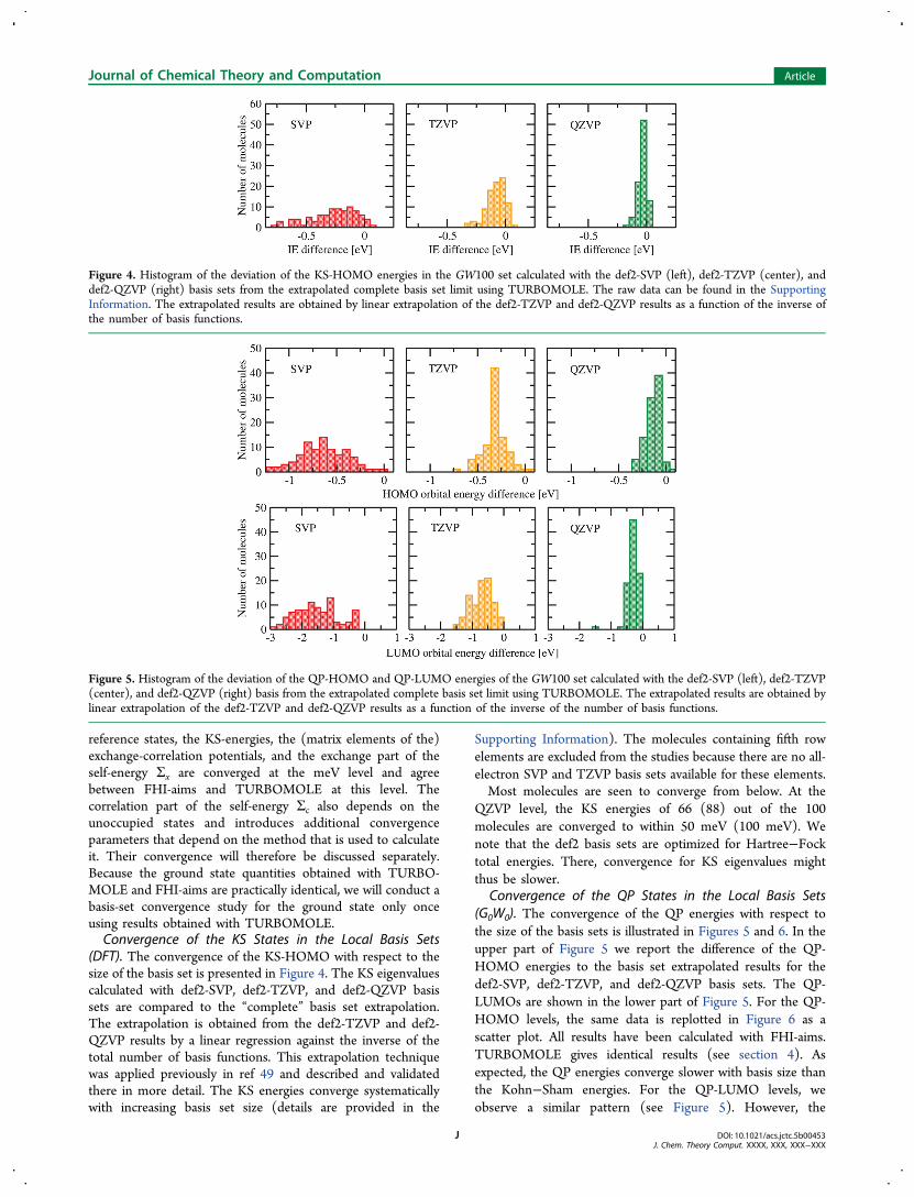
Convergence of the QP States in the Local Basis Sets(G0W0). The convergence of the QP energies with respect tothe size of the basis sets is illustrated in Figures 5 and 6. In theupper part of Figure 5 we report the difference of the QP-HOMO energies to the basis set extrapolated results for thedef2-SVP, def2-TZVP, and def2-QZVP basis sets. The QP-LUMOs are shown in the lower part of Figure 5. For the QP-HOMO levels, the same data is replotted in Figure 6 as ascatter plot. All results have been calculated with FHI-aims.TURBOMOLE gives identical results (see section 4). Asexpected, the QP energies converge slower with basis size thanthe Kohn−Sham energies. For the QP-LUMO levels, weobserve a similar pattern (see Figure 5). However, the

Figure 4. Histogram of the deviation of the KS-HOMO energies in the GW100 set calculated with the def2-SVP (left), def2-TZVP (center), anddef2-QZVP (right) basis sets from the extrapolated complete basis set limit using TURBOMOLE. The raw data can be found in the SupportingInformation. The extrapolated results are obtained by linear extrapolation of the def2-TZVP and def2-QZVP results as a function of the inverse ofthe number of basis functions.

Figure 5. Histogram of the deviation of the QP-HOMO and QP-LUMO energies of the GW100 set calculated with the def2-SVP (left), def2-TZVP(center), and def2-QZVP (right) basis from the extrapolated complete basis set limit using TURBOMOLE. The extrapolated results are obtained bylinear extrapolation of the def2-TZVP and def2-QZVP results as a function of the inverse of the number of basis functions.

Journal of Chemical Theory and Computation Article

DOI: 10.1021/acs.jctc.5b00453J. Chem. Theory Comput. XXXX, XXX, XXX−XXX

J

deviations are approximately a factor of 2 larger for each basisset.When comparing the QP results between the local orbital

codes FHI-aims and TURBOMOLE and the plane wave codeBerkeleyGW in the Results section, we will always use theextrapolated values. These will be referred to as “EXTRA”. Forthe QP energies, we estimate the error in the extrapolation bycomparing to a second extrapolation scheme, i.e., extrapolatingagainst 1/Cn

3 where Cn is the cardinal number of the basis set (2for SVP, 3 for TZVP, etc.). The mean absolute error is 0.04 forQP-HOMO and 0.1 for QP-LUMO. In the SupportingInformation, a systematic comparison against other basis sets(including Dunning’s correlation consistent basis sets113) isgiven for four typical molecules. In the Results section, theestimated errors are provided together with the extrapolatedresults.Auxiliary Basis Sets. The G0W0 implementations in

TURBOMOLE and FHI-aims make use of the resolution-of-identity (RI) technique to compute four-center Coulombintegrals of the type

∫φ φ φ φ

| =′ ′

| − ′|′ij kl

r r r r

r rr r( )

( ) ( ) ( ) ( )d di j k l

(29)

To avoid the numerical cost associated with the computationand storage of the (ij|kl) matrix, an auxiliary basis set {Pμ} isintroduced to expand the product of basis function pairs as

∑φ φ ≃μ

μμ

=

C Pr r r( ) ( ) ( )i j

N

ij1

aux

(30)

where Cijμ are the expansion coefficients, and Naux is the number

of auxiliary basis functions Pμ. The G0W0 equations can beconveniently rewritten employing eq 30 as described in detail inrefs 40, 49, and 114.In our experience, RI speeds up DFT calculations by an

order of magnitude in TURBOMOLE. For G0W0, thecomputational effort is reduced by an order of magnitude forcalculations with ∼100 basis functions. In addition, the scalingreduces from N5 to N4 or better (where N is the number ofatoms) up to 1000 basis functions.49 For G0W0 in FHI-aims, RI

is essential.40 The scaling of G0W0 in FHI-aims is always N4 orbetter.The auxiliary basis functions in TURBOMOLE are supplied

in a database.115,116 They are designed such that the RI-inducederror lies in the meV regime for DFT total energycalculations.116 An important difference for FHI-aims is thatthe auxiliary basis functions in FHI-aims are constructed on thefly40,114 and are not predefined as in TURBOMOLE.We define the G0W0 RI error as the difference between the

QP energies calculated with and without applying RI in all stepsof the calculation. This comparison is shown in Figure 7 for

TURBOMOLE using a subset of GW100. We observe thatG0W0 is more sensitive to the RI approximation than DFT withlocal or semi-local functionals. In an earlier study, we found fora smaller set of molecules that the G0W0 RI error for the QP-HOMO energies is below 0.1 eV.49 The same trend is observedhere (see Figure 7). Only very small systems, such as heliumand hydrogen, tend to have a larger G0W0 RI error of 0.24 and0.13 eV, respectively. In the FHI-aims calculations, theparameters for constructing the auxiliary basis sets are chosensuch that the quasi-particle energies agree with the RI-freeTURBOMOLE values to better than 1 meV compared for allsystems (see also Table 2). [All input and output files of theFHI-aims calculations are available at https://NOMAD-Repository.eu DOI: 10.17172/NOMAD/2015.11.03-1.]

Convergence in the Plane-Wave Basis. The BerkeleyGW59

package computes the dielectric function and self-energy withina plane-wave basis set. The input DFT-PBE eigenvalues arecomputed with the Quantum Espresso package117 with a plane-wave wave function cutoff defined such that the total DFT-PBEenergy is converged to <1 meV/atom. The wave functioncutoffs for all 100 molecules are provided in the SupportingInformation. Typical values between 50 (680) and 120 Ry(1633 eV) are sufficient, but in some cases, even 300 Ry (4082eV) are necessary. The molecules are placed in a large supercellthat is twice the size necessary to contain 99.9% of the chargedensity. To avoid spurious interactions between periodicimages at the G0W0 step, the Coulomb potential is truncatedat half of the unit cell length.59

The KS eigenvalues computed with Quantum Espresso agreewell with TURBOMOLE and FHI-aims (see Table S6 in the

Figure 6. Deviation of the QP-HOMO energies from the extrapolatedcomplete basis set limit for the def2-SVP, def2-TZVP and def2-QZVPbasis sets as a function of the inverse number of basis functions. Theresults have been obtained with TURBOMOLE.

Figure 7. G0W0 RI error of the QP-HOMO energies in theTURBOMOLE calculations compared to the reciprocal of the numberof basis functions (1/NBF). The RI error for the G0W0 calculations isdefined as the difference between the QP-energies calculated with andwithout applying the RI approach at all steps of the calculation.

Journal of Chemical Theory and Computation Article

DOI: 10.1021/acs.jctc.5b00453J. Chem. Theory Comput. XXXX, XXX, XXX−XXX

K

Supporting Information). In most cases, the deviation is wellbelow 0.1 eV, the mean absolute deviation is 0.048 eV with theextrapolated and 0.045 eV with the QZVP results. The largestdiscrepancies, on the order of 0.1 eV, occur almost exclusivelyin Fluor-containing molecules.As alluded to in section 3, we obtain the QP energies by

solving the QP equation (eq 7, repeated here for convenience)

ε ε= ϵ + ⟨ |Σ + Σ − | ⟩n v n( )n n x c nQP KS QP

xc (31)

We observe that Σx − vxc also differs by less than 50 meV forthe GW100 molecules between the three codes (see Table S6in the Supporting Information).The Response Function in the Local Basis. Because of the

compactness of the basis in TURBOMOLE and FHI-aims, theresponse function can be treated in the full Hilbert space of thedef2-QZVP basis for all molecules in GW100. Even for thesmallest molecules, the def2-QZVP basis describes a homoge-neous excitation spectrum up to 350 eV. For all molecules withmore than 4 electrons, the excitation spectrum ranges wellbeyond 800 eV. We tested that at least states up to 400 eV arerequired in the construction of Σ (i.e., in the sum over m in eq17) for all systems. The QP-HOMO energies are thenconverged to within 0.05 eV. For states with energies higherthan 400 eV, the denominator in eq 17 becomes large enoughto suppress further contributions.We mention this assessment here to estimate the

contribution of higher lying states in G0W0. In practice, wealways include all states of the Hilbert space spanned by thechosen basis set in our TURBOMOLE and FHI-aimscalculations.3.3. Treatment of Core Electrons. In the FHI-aims and

TURBOMOLE calculations, all electrons have been taken intoaccount explicitly at each step of the calculation. They areincluded fully in the KS and the G0W0 calculations and thusalso take part in the screening.3.3.1. Pseudopotentials. In the BerkeleyGW calculations, we

employed Troullier−Martins norm-conserving pseudopoten-tials.118 For all atoms except the transition metals, thepseudopotentials were taken from version 0.2.5 of theQuantum Espresso pseudopotential library.117 For Ti, Cu,and Ag, we found it necessary to include semicore states in thepseudopotential to properly describe the valence orbitals nearthe core.119 For Cu and Ag, we use the pseudopotentials ofHutter and co-workers120,121 in which 19 valence electrons aretreated explicitly. For Ti, we generated the pseudopotentialusing the FHI98pp package,87 treating 12 electrons as valence.The plane-wave cutoff is set such that total DFT energies areconverged to 10 meV/atom and the DFT HOMO energies areconverged to 50 meV for all molecules. As shown in Figure 8,the HOMO energies are converged to <5 meV for the majorityof the molecules (79 molecule). The error is computed as thedifference between the converged cutoff energy and a cutoff of120 Ry (1633 eV). For cases where the converged cutoff energyis determined to be greater than 120 Ry (1633 eV), the error isestimated as the difference between this value and a planewavecutoff, which is increased by 10 Ry (136 eV). The core radiicutoff for the pseudopotentials and the wave function cutoff forall 100 molecules are listed in the Supporting Information. Thissame planewave cutoff is used at the GW step.3.4. The Quasi-Particle Equation. The final technical step

of a G0W0 calculation is the solution of the quasi-particleequation. Once the G0W0 self-energy is obtained, the quasi-

particle energies εnQP are calculated by solving the diagonal

quasi-particle equation (eq 7, repeated here for convenience)

ε ε= ϵ + ⟨ |Σ − | ⟩n v n( )n n nQP KS QP

xc (32)

Here, ϵnKS are the Kohn−Sham eigenvalues (computed in PBE

in this work). Eq 32 is generally solved iteratively due to theinterdependence of the self-energy Σ(εnQP) and the quasi-particle energy εn

QP. In most cases, εnQP falls in a region in which

the self-energy has no poles, making it featureless and almostconstant. Then, the solution is unique in the region of interest,and eq 32 may even be linearized such that a single evaluationof Σ at the KS energy is sufficient and there is no iterationprocess. In BerkeleyGW GPP calculations, the quasi-particleequation is always linearized. This is justified because the GPPself-energy is smooth near the quasi-particle energy.In some cases, however, the initial KS energy is close to a

pole of Σ, and as a result, eq 32 has more than one solution.These solutions are relatively close in energy, which impliesthat the correction to the KS eigenvalue is not unique. Aschematic example is shown in Figure 9. In practice, mostavailable G0W0 codes search for only a single solution of thequasi-particle equation. Which solution is found depends onthe initialization and the type of the iterative procedure. Ingeneral, different codes might find different solutions to thenonlinear quasi-particle equation even though the self-energy issimilar. We expect all solutions to be physically relevant inprinciple. However, which one is actually physically relevantdepends, e.g., on the quasi-particle weight (i.e., the poleresidue), and furthermore may also depend on the physicalobservable one would like to study.Generically, one expects those solutions with the largest

quasi-particle peak Z/(ω − εnQP), the so-called Z-factor

ω=

− ⟨ |Σ | ⟩ω ω ε

∂∂ =

Zn n

1

1 ( )n

nQP (33)

Figure 8. Error in the computed DFT HOMO eigenvalues due to thechosen planewave cutoff. As noted in the text, the error is calculated asthe orbital energy difference for a calculation that employs the chosencutoff and 120 Ry (1633 eV) cutoff. If the converged cutoff is greaterthan or equal to 120 Ry (1633 eV), the error is determined as thedifference between the converged value and 10 Ry (136 eV) higherthan this value.

Journal of Chemical Theory and Computation Article

DOI: 10.1021/acs.jctc.5b00453J. Chem. Theory Comput. XXXX, XXX, XXX−XXX

L

to be most important. Especially very close to the poles, theslope of Σ at the quasi-particle energy is large, Z is small, andthe weight of the quasi-particle peak in the spectral function isreduced. The remaining weight is shifted to the other solutions,in the case of multiple solutions, or the incoherent background.Solutions that result from intersections with the almost verticallines when a pole in Σ changes sign are spurious in a sense. Forthe molecules considered here, these poles are very sharp, as wewill demonstrate in the Results section. The slope is thusalmost infinite and the corresponding weight will go to zero. Alesser Pade approximant or large damping η, as often applied ina full frequency treatment, will broaden the pole and can giverise to a nonvanishing spurious Z-factor. At this point, we willrefrain from further analysis of the role of the different solutionsfor physical observables. In this work, we ascribe the solutionwith the highest energy to the QP-HOMO.One may conclude now that states whose derivative of the

self-energy is large at the quasi-particle energy, i.e., that have asmall Z-factor, might lend themselves to multisolution behavior.If a small Z-factor is detected, it might indeed be necessary totest whether the solution of the quasi-particle equation actuallycorresponds to the highest in energy intersection between theΔ(ω) and Σ(ω). A small Z-factor, however, is not always anindicator of multisolution behavior. We will see examples of thisbelow.

4. RESULTS

In the following, we present our numerical assessment of theG0W0 implementations in TURBOMOLE, FHI-aims, andBerkeleyGW. We have chosen the energies of the highestoccupied molecular orbital (QP-HOMO, εH

QP) and lowestunoccupied molecular orbital (LUMO, εL

QP) as our mainobservables in this comparison. Both have a well-definedphysical meaning: εH

QP corresponds to the first verticalionization energy, and εL

QP is the electron affinity. For mostmolecules in the GW100 set, the quasi-particle equation yields aunique solution for QP-HOMO and QP-LUMO. However,four molecules exhibit the aforementioned multisolutionbehavior described in section 3.4. Section 4.1.1 reports allsolutions for these four molecules in detail. In the finalsubsection of the results section, we will then make acomparison to other G0W0 results that are available in theliterature.

4.1. Ionization Energies. Table 2 presents the G0W0@PBEQP-HOMO energies for the molecules of the GW100 set. (Fora subset of the molecules considered in this work, the G0W0@PBE ionization energies−evaluated with the three codes−havebeen reported in previous publications.37,40,49 The resultspresented in Table 2 show small numerical differences for someof these molecules. The deviations of these values to previouslypublished data are generally smaller than 0.1 eV and can bemainly attributed to the different (larger) basis sets employedin the present study. Furthermore, in the previous TURBO-MOLE calculations, we added an exchange-correlation kernelto the RPA response function and the quasi-particle equationwas linearized. The only molecule previously calculated withBerkeleyGW is benzene, for which there is no differencebetween our current and the previous calculation.) For brevity,we have introduced the following abbreviations in this section:AIMS-2P for a two pole fit in FHI-aims and AIMS-P16 andAIMS-P128 for a 16 and 128 parameter Pade fit in FHI-aims,respectively, BGW-GPP and BGW-FF for the generalizedplasmon model and the full-frequency treatment in Berke-leyGW, respectively, and TM-RI and TM-noRI for the RI andthe RI-free treatment in TURBOMOLE. respectively. EXTRAdenotes extrapolated local orbital results obtained byextrapolating the def2-TZVP and QZVP values calculatedusing FHI-aims (see section 3.2). The TM-noRI and the BGW-FF calculations are computationally very demanding. They havetherefore only been performed for subsets of the GW100 set(see Tables 2 and 5).The absolute values of the differences of the approaches used

in this work are reported in Figure 10 for all moleculesconsidered in this work. The FHI-aims and TURBOMOLEresults are compared at the QZVP level, and the BerkeleyGWresults are compared to the extrapolated results. The AIMS-P16and TM-noRI QP energies (green shading) generally differ byless than 1−2 meV. There are, however, some molecules forwhich we observe a larger discrepancy. In these cases, weobserve a QP weight Z in the range between 0.6 and 0.8. AIMS-P16 is slightly less accurate in these cases. For the systems forwhich we observe the multisolution behavior (ozone (index81), boron nitride (index 65), beryllium oxide (index 84), andmagnesium oxide (index 85)), the quasi-particle equation forthe QP-HOMO is solved close to a pole of the self-energy. Asalluded to in section 3.4, this leads to multiple solutions of the

Figure 9. Schematic of a graphical solution of the quasi-particle equation (eq 32). All intersections of the red line with the correlation part of the self-energy (black line) are solutions of the quasi-particle equation. The left panel shows the most common situation with a clear single solution near theKS starting point; the right panel shows the situation that can lead to multiple solutions.

Journal of Chemical Theory and Computation Article

DOI: 10.1021/acs.jctc.5b00453J. Chem. Theory Comput. XXXX, XXX, XXX−XXX

M

quasi-particle equation even though the underlying self-energiesshow only minor numerical differences. These cases will bediscussed separately in section 4.1.1.As is also seen in Table 2 and Figure 10, slightly larger

discrepancies are observed for the other implementations (seered and yellow shading in Figure 10). AIMS-2P and TM-RIyield values that are generally within 0.1 eV of the AIMS-P16and TM-noRI results. Similarly, the BGW-FF QP energiesagree with AIMS-P16 values within 0.2 eV and BGW-GPPwithin 0.5 eV.Table 3 condenses the information given in Figure 10 by

reporting the mean deviation (MD) and mean absolute

deviation (MAD) of the QP-HOMO energies obtained fromthe different G0W0 calculations. The mean deviations reportedin Table 3 show that TM-RI tends to underestimate QP-HOMO, whereas the generalized plasmon pole model leads tolarger QP-HOMO values, overestimating the full-frequency-determined QP-HOMO for all systems.The most important conclusion that can be drawn from

Tables 2 and 3 is that the AIMS-P16 and TM-noRI resultsagree to within 3 meV; the numerical aspects in theseconsiderably different implementations are under control. Itfurther shows that the analytic continuation for quasi-particleenergies is very accurate, provided that a Pade fit is used andthe number of parameters is converged explicitly. We willtherefore use AIMS-P16 and AIMS-P128 to extrapolate theQP-HOMO energies to the complete basis set limit, which isalso shown in Table 2 in the column EXTRA. This columnpresents our main result, converged benchmark numbers forthe GW100 set.There is a difference of ∼0.5 eV between the ionization

energies from BGW-GPP and TM or AIMS as shown in Table3. The comparison with BGW-FF shows that the majority of

these differences arise from the GPP approximation. For the 18molecules we tested explicitly (discounting possible deviationsarising from the multiple solution behavior), BGW-FF andEXTRA agree to better than 0.2 eV.

4.1.1. Multiple Solutions of the Quasi-Particle Equation.The quasi-particle energies listed in Table 2 have been obtainedfrom the solution of the nonlinear quasi-particle (eq 32). Asalluded to before, the solution for the QP-HOMO (and QP-LUMO) is unique for the majority of the systems consideredhere. However, for the QP-HOMO of ozone, boron nitride,magnesium oxide, and beryllium oxide, we find multiplesolutions. Figure 11 illustrates the behavior for ozone for the

different calculations. An analogous plot for magnesium oxide isshown in section 5.1, and plots for boron nitride and berylliumoxide are reported in the Supporting Information. Thesolutions of the QP equation are the intersections of the redline with the self-energy curves. Table 4 reports all solutions wefind for the four multisolution molecules.It should be noted that, technically speaking, each solution of

the quasi-particle equation is potentially physically relevant.However, at least two mechanisms can be identified, whereas inpractice usually not more than one solution needs to beconsidered. First, in cases with strong broadening, secondaryintersections are suppressed, see, for example, the blue trace inFigure 11. Second, even if the broadening is weak, the slope ofthe self-energy at the intersection point (i.e., the quasi-particleweight) will be different, favoring in general one point againstall others. Only in intermediate situations, as appears to be thecase with ozone, for example, could two or more solutionssurvive.

4.2. Electron Affinities. In Table 5 we report the G0W0@PBE electron affinities for the molecules of the GW100 set.Again, we present AIMS-2P, AIMS-P16, BGW-GPP, BGW-FF,TM-noRI, and TM-RI results.The absolute value of the difference between the various

calculated electron affinities are reported in Figure 12.

Figure 10. Absolute difference between QP-HOMO energiescalculated with the different G0W0 implementations. The FHI-aimsand TURBOMOLE results are compared at the QZVP level. TheBerkeleyGW results are compared to the extrapolated values. Theaverages of the absolute deviations are shown as horizontal lines.

Table 3. Mean Deviation (MD) and Mean AbsoluteDeviation (MAD) between the QP-HOMO EnergiesPresented in Table 2

MD (eV) MAD (eV)

AIMS-P16 - AIMS-2P −0.0014 0.1250AIMS-P16 - TM-RI 0.0456 0.0467AIMS-P16 - TM-noRI −0.0005 0.0032EXTRA - BGW-GPP −0.4990 0.5002EXTRA - BGW-FF 0.2030 0.2143

Figure 11. Comparison of the energy-dependent correlation part ofthe self-energy Σc(ε) calculated with the three different codes usingdifferent procedures for ozone. “TM-5” and “TM-3” indicateTURBOMOLE results calculated with imaginary shifts of η = 10−3

and 10−5 Hartree, respectively. The intersections of these curves withthe (red) line ω − ϵKS + Vxc − Σx correspond to the solutions of theQP equation.

Journal of Chemical Theory and Computation Article

DOI: 10.1021/acs.jctc.5b00453J. Chem. Theory Comput. XXXX, XXX, XXX−XXX

N

The analysis of the deviations in Table 6 and Figure 12shows trends similar to those observed for εH

QP in section 4.1.Again, the agreement between the TM-noRI and AIMS-P16electron affinities is on the order of a few meV. The TM-RIG0W0 implementation yields electron affinities that aregenerally within 14 meV from the TM-noRI and AIMS-P16values. One may conclude from this that QP energies ofoccupied states are more sensitive to the RI approximation thanthose of unoccupied states.In the comparison between the extrapolated and BGW data,

we observe a significant difference between systems with abound and unbound LUMO state. In the case of a boundLUMO state, the agreement between the EXTRA values andBGW results is similar to that observed for the occupied states.For the unbound LUMOs, the agreement can be far off. Here,the local orbital description of the unbound states clearly is notwell-converged. It is noted, however, that the convergence isthe worst for small systems. Most molecules with more thanfour none-hydrogen atoms show a small deviation also forunbound LUMOs.4.3. Literature Comparison. 4.3.1. Comparison with

Plane-Wave Results. A subset of the GW100 molecules(C2H4O is present in both sets; in GW100, this is acetaldehyde,whereas in Pham et al.’s set, this is ethylene oxide) haspreviously been calculated by Pham et al. using a plane-wavebasis set.38,45 The diagonal quasi-particle equation was solved as

in the present work. Moreover, the analytic structure of the self-energy was taken into account consistently. These results arehence fully comparable to the results of the present paper. Forseven out of 12 of the molecules in the intersecting subset, weobserve an agreement within ∼0.1 eV of our extrapolatedresults. The molecules containing fluorine show a somewhatlarger discrepancy and so do ozone and pyridine (up to 0.5 eV).For ozone, the slope of the self-energy around the quasi-particleenergy is steep, which implies a low quasi-particle weight (seesection 4.1.1) and furthermore exhibits multisolution behavioras discussed previously and in section 4.1.1. In pyridine, theself-energy also exhibits a relatively large slope of 0.35.However, no multisolution behavior aggravates the solutionof the quasi-particle equation.DNA bases have been studied by Qian et al.31 They used a

plane-wave basis in combination with a Wannier-typeoptimized basis for the response function. The diagonalquasi-particle equation was solved as in the present work, andthe self-energy was calculated using the analytic continuation.They estimated that their results are accurate to within 0.1 eV.Our extrapolated results for G, A, C, T lie approximately 0.2 eVlower in energy (0.4 eV for uracil). There are two possiblecauses for the observed deviation. First, the comparison ofextrapolated results to none-extrapolated results, which tends tolower the extrapolated results. The second cause is thecomparison of all-electron to froze-core results; increasing thenumber of valence electrons increases the screening. Thisreduces the absolute size of the (in general positive)contribution of the correlation part of the self-energy andhence lowers the QP energies. Both effects thus point in thedirection of the observed deviation.

4.3.2. Comparison with Local-Orbital Results. Recently,several local-orbital G0W0 implementations have emerged. Wehave included the G0W0@PBE values reported with thesecodes29,30,32,33,40,41,44,47−50 in Table 7. We often observenumerical differences that are larger than 0.1 eV and, forsome systems, on the order of 1 eV. For example, the G0W0@PBE ionization energy of the CO2 molecule has already beenstudied in several other works.29,40,47,49 The reported valuesspan a range of almost 1 eV (12.8−13.6 eV, the experimentalionization energy being 13.78 eV122). For other systems, e.g.,N2 and NH3, the published G0W0@PBE ionization energies arealso distributed in a similar energy range.We attribute the large spread to the different basis function

choices (Gaussian, molecular orbital, etc.) and sizes (triple-ζ,quadruple-ζ, etc.) and the fact that no extrapolation to thecomplete basis set limit has been performed. The differenttreatments of the frequency dependence also play a role. Theresults reported in this work allow us to estimate the impact ofthese approximations. For instance, Figure 10 illustrates thatthe error of a two-pole analytic continuation is mostly smallerthan 0.12 eV. Conversely, Figure 6 indicates that the basis setsize has a considerable impact on the ionization energies. Evenfor the relatively large QZVP basis, the QP-HOMO energiesare underestimated by ∼0.12 eV on average.Another factor that may affect the comparison with the

published G0W0 ionization energies is the way in which thequasi-particle equation is solved. The quasi-particle energiesmay be determined either from the iterative solution of eq 32or, alternatively, from the linearized quasi-particle equation(see, for example, ref 136.). Looking at our CO2 example, it islinearized in refs 29, 47, and 49 and solved in ref 40. We find

Table 4. Solutions of the Quasi-Particle Equation for theQP-HOMO Level of Ozone, Boron Nitride, BerylliumOxide, and Magnesium Oxide for the Different Calculationsa

calculation left center right

BNBGW-GPP −12.19BGW-FF −9.68AIMS-2P −11.19AIMS-P16 −11.15AIMS-P128 −11.67 −11.46 −11.03TM −11.67 −11.42 −11.00

O3

BGW-GPP −12.73BWG-FF −12.00AIMS-2P −11.91AIMS-P16 −11.96 −11.63 −11.39AIMS-P128 −11.96 −11.63 −11.39TM −11.95 −11.62 −11.39

BeOBGW-GPP −10.50BGW-FF −9.68 −8.64 −8.45AIMS-2P −9.35AIMS-P16 −9.07AIMS-P128 −9.63 −8.88 −8.58TM −9.63 −8.86 −8.62

MgOBGW-GPP −8.369BGW-FF −7.08AIMS-2P −7.03AIMS-P16 −6.79AIMS-P128 −7.11 −6.95 −6.68TM −7.09 −6.91 −6.66

aThe numbers in boldface are the solutions as reported by the specificcode (as reported solution). In Table 2, we always report the solutionwith the highest energy.

Journal of Chemical Theory and Computation Article

DOI: 10.1021/acs.jctc.5b00453J. Chem. Theory Comput. XXXX, XXX, XXX−XXX

O

Table 5. LUMO Energies Analagous to Table 2a

name formula AIMS-2P AIMS-P16 BGW-GPP BGW-FF TM-RI TM-noRI EXTRA(ERR) exp.

1 helium He 11.01 11.01 0.44 11.07 11.012 neon Ne 11.63 11.64 0.13 11.65 11.643 argon Ar 8.08 8.11 −0.69 8.12 8.114 krypton Kr 7.61 7.63 −0.80 7.62 7.635 xenon Xe 7.92 7.98 0.23 7.96 7.986 hydrogen123 H2 3.50 3.50 0.26 3.50 3.50 3.30(0.52)7 lithium dimer123 Li2 −0.67 −0.63 −0.79 −0.61 −0.63 −0.75(0.04)8 sodium dimer123 Na2 −0.61 −0.55 −0.59 −0.50 −0.54 −0.66(0.7) 0.54*9 sodium tetramer124 Na4 −1.09 −1.01 −1.17 −0.99 −1.01 −1.15(0.9) 0.91*10 sodium hexamer124 Na6 −1.07 −0.97 −1.08 −0.94 −0.97 −1.13(0.10)11 potassium dimer123 K2 −0.61 −0.65 −0.72 −0.62 −0.65 −0.75(0.05) 0.50*12 rubidium dimer125 Rb2 −0.63 −0.62 −0.74 −0.62 0.50*13 nitrogen123 N2 2.41 2.45 2.00 2.47 2.45 2.12(0.09)14 phosphorus dimer123 P2 −0.82 −0.72 −1.21 −0.70 −0.72 −1.08(0.08) 0.63*15 arsenic dimer123 As2 −0.92 −0.85 −1.12 −0.86 −0.85 −1.52(0.35) 0.74*16 fluorine123 F2 −0.88 −0.70 −0.41 −0.97 −0.63 −0.70 −1.23(0.14)17 chlorine123 Cl2 −0.98 −0.89 −1.56 −0.85 −0.89 −1.40(0.12)18 bromine123 Br2 −1.54 −1.40 −1.93 −1.41 −1.40 −1.96(0.29)19 iodine123 I2 −1.81 −1.68 −2.17 −2.1620 methane123 CH4 2.42 2.45 0.25 2.48 2.45 2.03(0.35)21 ethane123 C2H6 2.27 2.29 0.32 2.32 2.29 1.93(0.24)22 propane126 C3H8 2.16 2.19 0.35 2.23 2.19 1.87(0.19)23 butane123 C4H10 2.12 2.14 0.36 2.18 1.83(0.17)24 ethylene123 C2H4 1.94 2.02 1.91 2.04 2.02 1.82(0.09)25 acetylene123 C2H2 2.81 2.86 0.19 2.88 2.86 2.56(0.04)26 tetracarbon127 C4 −3.03 −2.94 −3.20 −2.93 −3.15(0.06) 3.88*27 cyclopropane123 C3H6 2.42 2.45 0.35 2.48 2.45 1.96(0.21)28 benzene123 C6H6 0.97 1.09 1.16 1.10 0.89(0.03)29 cyclooctatetraene128 C8H8 −0.01 0.06 0.04 0.07 −0.12(0.02) 0.6530 cyclopentadiene123 C5H6 0.98 1.04 1.02 1.06 0.85(0.04)31 vinyl fluoride123 C2H3F 2.04 2.15 2.12 2.08 2.17 2.15 1.88(0.03)32 vinyl chloride123 C2H3Cl 1.32 1.42 1.20 1.44 1.44 1.17(0.03)33 vinyl bromide123 C2H3Br 1.35 1.38 1.25 1.40 1.11(0.01)34 vinyl iodide123 C2H3I 0.82 0.89 0.47 0.8435 tetrafluoromethane123 CF4 4.34 4.41 0.32 4.42 4.41 3.88(0.14)36 tetrachloromethane123 CCl4 −0.08 −0.01 −0.64 0.02 −0.54(0.13)37 tetrabromomethane123 CBr4 −1.14 −1.08 −1.43 −1.08 −1.56(0.29)38 tetraiodomethane123 CI4 −2.22 −2.14 −2.43 −2.1139 silane123 SiH4 2.48 2.51 0.09 2.53 2.51 2.26(0.19)40 germane123 GeH4 2.12 2.30 0.04 2.31 2.30 1.85(0.18)41 disilane123 Si2H6 1.65 1.69 0.23 1.72 1.51(0.10)42 pentasilane127 Si5H12 0.07 0.16 −0.08 0.19 0.00(0.07)43 lithium hydride123 LiH −0.11 −0.07 −0.37 −0.06 −0.07 −0.16(0.09) 0.34*44 potassium hydride123 KH −0.17 −0.18 −0.56 −0.16 −0.18 −0.32(0.01)45 borane123 BH3 0.05 0.12 −0.06 0.12 0.12 0.03(0.05) 0.04*46 diborane(6)123 B2H6 0.78 0.84 0.70 0.85 0.84 0.74(0.07)47 ammonia123 NH3 2.28 2.31 0.24 2.33 2.31 2.00(0.20)48 hydrazoic acid123 HN3 1.34 1.40 1.38 1.43 1.40 1.10(0.04)49 phosphine123 PH3 2.46 2.50 0.03 2.52 2.50 2.26(0.14)50 arsine123 AsH3 1.84 2.32 −0.13 2.34 2.32 1.94(0.09)51 hydrogen sulfide123 SH2 2.52 2.56 −0.35 2.59 2.56 2.25(0.11)52 hydrogen fluoride123 FH 2.51 2.54 0.26 2.55 2.54 2.04(0.07)53 hydrogen chloride123 ClH 2.00 2.06 −0.45 2.09 2.06 1.53(0.06)54 lithium fluoride123 LiF 0.09 0.09 −0.58 0.09 0.09 −0.01(0.01)55 magnesium fluoride123 F2Mg −0.18 −0.14 −1.22 −1.18 −0.14 −0.14 −0.31(0.06)56 titanium tetrafluoride123 TiF4 −0.59 −0.60 −0.66 −0.57 −1.06(0.13) 2.5057 aluminum fluoride123 AlF3 0.07 0.16 −0.61 0.17 0.16 −0.23(0.10)58 boron monofluoride123 BF 1.06 1.22 0.89 1.24 1.22 1.05(0.05)59 sulfur tetrafluoride129 SF4 0.25 0.38 0.00 0.42 0.38 −0.10(0.13)60 potassium bromide123 BrK −0.30 −0.31 −0.91 −0.31 −0.31 −0.42(0.06) 0.64*61 gallium monochloride123 GaCl −0.04 −0.02 −0.31 −0.01 −0.02 −0.39(0.15)

Journal of Chemical Theory and Computation Article

DOI: 10.1021/acs.jctc.5b00453J. Chem. Theory Comput. XXXX, XXX, XXX−XXX

P

that the ionization energies obtained from these twoapproaches may differ by up to 0.5 eV.In summary, we believe that deviations up to a few hundred

meV can be explained by the technical differences in the G0W0

implementations discussed above. We mention that the resultsof Rostgaard et al.29 deviate in 4 out of 22 cases by ∼1 eV ormore (up to 2 eV), which seems hard to reconcile with ourgeneral findings.4.4. Comparison to Experimental Values. In this work,

the focus is on methodology; we establish a G0W0@PBEbenchmark that holds (with certain bounds) irrespective ofhow the G0W0 equations have been implemented. Residualdiscrepancies to experimental data persist, which are typicallyseveral hundred meV (see Table 8). Our work strongly suggeststhat on the theory side these discrepancies reflect (i) theneglect of self-consistency and (ii) vertex corrections.

For some classes of molecules, an informed choice of thestarting point, e.g., B3LYP, PBE0, or static COHSEX instead ofPBE, could lead to a reduction of the discrepancies toexperiment by factors of order unity (see, for example, refs43 and 137). However, corrections that are applicable to broadsystem classes and that can be systematically improved uponcan probably not be achieved in this way. Our table also showsa comparison between the simplifying GPP model andexperimental data. The comparison is favorable, at first sight,which at this point is not fully understood and a matter ofongoing investigation.63

5. DISCUSSIONAs discussed in section 3.2, both the KS energies and theexchange part of the self-energy are well converged. Moreover,we have already discussed in section 3.2 the errors introducedby the finite basis set and additional computational

Table 5. continued

name formula AIMS-2P AIMS-P16 BGW-GPP BGW-FF TM-RI TM-noRI EXTRA(ERR) exp.

62 sodium chloride123 NaCl −0.39 −0.39 −1.38 −0.39 −0.39 −0.42(0.01) 0.73*63 magnesium chloride123 MgCl2 −0.52 −0.43 −1.30 −0.43 −0.43 −0.68(0.08)64 aluminum iodide123 AlI3 −0.87 −0.80 −1.23 −0.7865 boron nitride123 BN −3.93 −3.88 −3.99 −3.93 −3.95 −3.95(0.02) 3.16*66 hydrogen cyanide123 NCH 2.54 2.58 2.47 2.60 2.58 2.22(0.02)67 phosphorus mononitride123 PN −0.30 −0.20 −0.65 −0.18 −0.20 −0.59(0.10)68 hydrazine123 H2NNH2 1.96 1.99 0.33 0.35 2.02 1.99 1.68(0.14)69 formaldehyde123 H2CO 0.89 0.96 0.93 0.99 0.96 0.71(0.03)70 methanol123 CH4O 2.22 2.25 0.42 2.27 2.25 1.81(0.19)71 ethanol130 C2H6O 2.04 2.08 0.44 2.10 1.67(0.17)72 acetaldehyde123 C2H4O 0.99 1.05 1.10 1.08 0.83(0.05)73 ethoxy ethane131 C4H10O 2.07 2.10 0.36 2.13 1.70(0.17)74 formic acid123 CH2O2 1.85 1.91 1.91 1.94 1.91 1.59(0.00)75 hydrogen peroxide123 HOOH 2.21 2.35 2.17 1.95 2.40 2.35 1.95(0.05)76 water123 H2O 2.33 2.37 0.26 2.38 2.38 2.01(0.16)77 carbon dioxide123 CO2 2.45 2.50 0.25 0.28 2.50 2.50 0.93(0.42)78 carbon disulfide123 CS2 −0.30 −0.20 −0.43 −0.16 −0.20 −0.55(0.09) 0.5879 carbon oxide sulfide123 OCS 1.14 1.21 0.94 1.03 1.25 1.22 0.83(0.10) 0.4680 carbon oxide selenide123 OCSe 0.80 0.87 0.73 0.90 0.52(0.13)81 carbon monoxide123 CO 0.58 0.67 0.40 0.70 0.67 0.37(0.08) 1.3382 ozone123 O3 −2.41 −2.30 −2.59 −1.87 −2.23 −2.30 −2.69(0.11) 2.10*83 sulfur dioxide123 SO2 −1.12 −1.00 −1.24 −0.95 −1.00 −1.49(0.12) 1.11*84 beryllium monoxide123 BeO −2.34 −2.56 −2.80 −2.48 −2.49 −2.72(0.04)85 magnesium monoxide123 MgO −2.01 −1.89 −2.08 −1.87 −2.13(0.09)86 toluene123 C7H8 0.94 1.01 0.95 1.03 0.83(0.03)87 ethylbenzene127 C8H10 0.97 1.04 0.96 1.06 0.87(0.04)88 hexafluorobenzene126 C6F6 0.61 0.66 −0.21 0.68 0.36(0.08) 0.7089 phenol123 C6H5OH 0.88 0.96 0.93 0.97 0.74(0.02)90 aniline123 C6H5NH2 1.06 1.15 1.13 1.16 0.94(0.03)91 pyridine123 C5H5N 0.41 0.51 0.50 0.53 0.30(0.01)92 guanine127 C5H5N5O 0.72 0.74 0.42 0.77 0.46(0.02)93 adenine127 C5H5N5O 0.42 0.47 0.48 0.49 0.21(0.01) −0.54*94 cytosine127 C4H5N3O 0.21 0.26 0.26 0.28 0.01(0.01)95 thymine127 C5H6N2O2 0.01 0.06 0.00 0.08 −0.18(0.01) −0.29*96 uracil127 C4H4N2O2 −0.07 0.01 −0.03 0.03 −0.25(0.01) −0.22*97 urea132 CH4N2O 1.60 1.62 0.25 1.64 1.17(0.02)98 silver dimer133 Ag2 −1.06 −1.05 −1.47 −1.20 1.10*99 copper dimer134 Cu2 −1.21 −0.92 −1.44 −0.75 −0.76 −1.23(0.08) 0.84*100 copper cyanide123 NCCu −1.84 −1.65 −2.08 −1.64 −1.85(0.05) 1.47*

aThe experimental electron affinities marked with * are laser photoelectron spectroscopy values. We note that the QP-LUMOs of the single atoms inthe GW100 set (He−Xe) exhibit such a strong dependence on the basis set that a controlled extrapolation is not possible within the SVP, TZVP, orQZVP series. As before, no extrapolated values are presented for molecules containing fifth row elements because SVP and TZVP all-electron basissets are not available.

Journal of Chemical Theory and Computation Article

DOI: 10.1021/acs.jctc.5b00453J. Chem. Theory Comput. XXXX, XXX, XXX−XXX

Q

approximations, such as RI and the freezing of core states. Inthis section, we discuss the differences between the QP energiesreported in Tables 2 and 5 that originate from the correlationpart of the GW self-energy. We start by discussing theappearance of multiple solutions of the QP equation and theirimpact on the QP energies. Then, we discuss the aspects thatrelate to different approaches to treat the frequency depend-ence of the self-energy.5.1. Multiple Solutions of the QP Equation. For four

molecules, ozone, boron nitride, beryllium oxide, andmagnesium oxide, we found multiple solutions with comparableenergy for the QP-HOMO level. To illustrate this behavior, weshowed the correlation part of the G0W0@PBE self-energy forozone in Figure 11. In Figure 13, we show that of magnesiumoxide. Similar plots for boron nitride and beryllium oxide areprovided in the Supporting Information. For boron nitride,Δ(ω) crosses one pole of Σ(ω), which results in threesolutions. For ozone, beryllium oxide, and magnesium oxide,we obtain five solutions.Inspection of Figures 11 and 13 confirms that the

multisolution behavior typically emerges when the intersection

is close to poles in the self-energy. For BrK, LiH, KH, coppercyanide, and Cu2, we also observe large self-energy derivatives(small Z-factors), but the poles are not close enough to thesolution of the quasi-particle equation to give rise to multiplesolutions. An example is show in Figure 14 for copper cyanide.The slope of the self-energy is large but rather constantbetween the KS energy and the QP energy. Any Newton−Raphson-like algorithm to iterate the QP equation willconverge to a unique QP energy when started at the KSenergy. This QP energy is, however, close to a pole, hence smalldifferences in the self-energy calculated by the differentapproaches do result in changes in the final value. Thisbehavior differs from the case of magnesium oxide, for example,where the first iteration step takes the algorithm to the otherside of the first pole.Figures 11 and 13, as well as Table 4, illustrate that the

occurrence of multiple solutions strongly depends on thefrequency treatment of the G0W0 implementation. In general,the GPP approach and the two pole analytic continuation givesrise to a self-energy that has too few poles or poles that areconsiderably broadened. Additionally, the GPP approximationshifts the self-energy poles away from the quasi-particleenergies, resulting in higher predicted G0W0 quasi-particleenergies. The result is a slowly varying self-energy with a uniquesolution to the quasi-particle equation in the energy region ofinterest. For many systems (including many of the molecules inGW100), the true poles of Σ are sufficiently far away from thequasi-particle energies or several poles merge into a broad polewith a gently sloped self-energy in the energy region of interest.In these cases, the GPP model and the two pole analyticcontinuation can be expected to agree well with the analyticand numerical full frequency methods (see also section 5.2).In the case of multiple solutions, the solution that is reported

by the code depends on the iterative solver that is employed forthe QP equation. The solver in TURBOMOLE is constructedto always find the solution with the largest quasi-particle weight,i.e., the smallest derivative. In FHI-aims, a simple iteration isused, which sometimes yields a different solution. InBerkeleyGW, the QP equation is linearized in the case ofGPP and solved by graphically finding the point where ϵKS + Σ− VXC is equivalent to ϵQP in the case of FF.

5.2. Pade, Two-Pole, and Plasmon Pole Approxima-tions. For most systems, the solutions of the diagonal QPequation (eq 32) are found in a region in which the self-energyis rather flat, i.e., ∂Σ/∂ε is small and the quasi-particle weight

=ε− ∂Σ ∂Z 1

1 /is close to unity. In these cases, the self-energy is

only evaluated in an energy region in which there are no polesnearby. For this purpose, a simple approximation for the energydependence of Σ, such as the two-pole analytic continuation,may provide quasi-particle energies converged within 0.2 eV, asthe data reported in Tables 2 and 5 indicate. This is furtherillustrated in Figure 15, where we report the difference betweenthe AIMS-2P and TM-noRI ionization energies (left panel) andbetween BGW-GPP and EXTRA (right panel), as a function ofΣ′ = ∂Σ/∂εFor small values of Σ′ (−0.5<Σ′ < 0), the deviation between

AIMS-2P and TM-noRI is consistently below 0.2 eV. In thiscase, the two-pole analytic continuation tends to overestimatethe ionization energies by ∼0.1 eV on average. However, for Σ′< −0.5, AIMS-2P systematically underestimates the ionizationenergies by 0.4−0.5 eV as compared to TM-noRI.138

Figure 12. Absolute difference between QP-LUMO energiescalculated with the different G0W0 implementations. The FHI-aimsand TURBOMOLE results are compared at the QZVP level. TheBerkeleyGW results are compared to the extrapolated values. Theaverages of the absolute deviations are shown as horizontal lines.

Table 6. Mean Deviation (MD) and Mean AbsoluteDeviation (MAD) between the QP-LUMO EnergiesPresented in Table 2

MD (eV) MAD(eV)

AIMS-P16 - AIMS-2P 0.0652 0.0710AIMS-P16 - TM-RI −0.0143 0.0302AIMS-P16 - TM-noRI −0.0035 0.0061EXTRA - BGW-GPP 0.4399 0.6902EXTRA - BGW-GPP (bound) 0.0682 0.0725EXTRA - BGW-FF 0.3133 0.4388

Journal of Chemical Theory and Computation Article

DOI: 10.1021/acs.jctc.5b00453J. Chem. Theory Comput. XXXX, XXX, XXX−XXX

R

Molecules that present large derivatives ∂Σ/∂ϵ for the QP-HOMO level are, for instance, BrK, LiH, KH, Cu2, NCCu, O3,BN, BeO, and MgO. Here, the quasi-particle equation hassolutions close to a pole of the self-energy, as illustrated inFigures 11 and 13. As a consequence, the resolution of thepole-structure of the self-energy, as achieved by differentmethods, now matters more. For O3, BeO, and MgO, AIMS-P16 provides enough fitting parameters. Conversely, for BNand CNCu, it is necessary to increase the number of Pade parameters up to 128 to describe the poles of the self-energysufficiently well, as illustrated in Figures 11 and 13 and Table 4.

Very smooth self-energies result from plasmon-pole modelsfor the response function. Besides the “flattening” of thecorrelation part of the self-energy, we also observe an overalldecreased correlation part of the self-energy (see Figures 11and 13) that is not present in the 2-pole self-energy.

5.3. Numerical Full Frequency Integration. In contrastto imaginary frequency treatments and plasmon pole models, afull frequency treatment can in principle be converged to theexact analytic G0W0 self-energy by increasing the density of thefrequency grid. (The Pade approximation could, in principlefrom a mathematical point of view, also be converged fully to

Table 7. G0W0@PBE Literature Values for QP-HOMO Energies Compared to the BGW-GPP and Extrapolated Data from thisStudya

name formula BGW-GPP EXTRAPham et al.45

(PW)Bruneval et al.47

(LO)Rostgaard et al.29

(LO)Qian et al.31

(PW) other

lithium dimer Li2 −5.43 −5.05 −5.12 −4.4 −5.1418

sodium dimer Na2 −5.03 −4.88 −4.89 −4.7 −5.116

sodium tetramer Na4 −4.34 −4.14 −4.2516

sodium hexamer Na6 −4.47 −4.34 −4.1616

potassium dimer K2 −4.02 −4.08 −3.8418

nitrogen N2 −15.43 −15.05 −14.98 −15.7phosphorus dimer P2 −10.66 −10.38 −10.12 9fluorine F2 −15.59 −15.10 −15.19 −16.2chlorine Cl2 −11.85 −11.31 −11.16 −11.5methane CH4 −14.28 −14.00 −14.03 −14.4 −14.3135

propane C3H8 −12.05 −11.89 −11.84butane C4H10 −11.73 −11.59 −11.58ethylene C2H4 −10.68 −10.40 −10.37 −9.6acetylene C2H2 −11.35 −11.09 −11.08 −11.2cyclopropane C3H6 −10.93 −10.65 −10.6benzene C6H6 −9.21 −9.10 −9.04 −9.0399

tetrafluoromethane CF4 −15.96 −15.60 −15.38tetrachloromethane CCl4 −11.77 −11.21 −11.22silane SiH4 −12.77 −12.40 −12.4 −12.4 −12.3099

disilane Si2H6 −10.80 −10.41 −10.38 −11.3lithium hydride LiH −7.85 −6.58 −7.07 −8ammonia NH3 −10.93 −10.39 −10.5 −10.6 −10.719

phosphine PH3 −10.79 −10.35 −10.21 −10hydrogen sulfide SH2 −10.64 −10.13 −9.9hydrogen chloride ClH −12.97 −12.36 −12.35lithium fluoride LiF −11.84 −10.27 −10.61 −12aluminum fluoride AlF3 −15.11 −14.48 −14.34sodium chloride NaCl −9.60 −8.43 −8.43 −8.8hydrogen cyanide NCH −13.87 −13.32 −13.2hydrazine H2NNH2 −9.78 −9.37 −9.87 −9.5formaldehyde H2CO −11.02 −10.46 −10.51hydrogen peroxide HOOH −11.58 −11.10 −11.02 −11.1water H2O −12.75 −12.05 −12.15 −11.9carbon dioxide CO2 −13.81 −13.46 −13.32 −13.6carbon disulfide CS2 −10.37 −9.95 −9.89carbon oxide sulfide OCS −11.49 −11.11 −11.01carbon monoxide CO −14.33 −13.71 −13.55 −13.9 −14.119

ozone O3 −13.05 −11.49 −12.2sulfur dioxide SO2 −12.55 −12.06 −11.83 −11.7pyridine C5H5N −9.50 −9.17 −9.54guanine C5H5N5O −7.92 −7.87 −7.64adenine C5H5N5O −8.35 −8.16 −7.99cytosine C4H5N3O −8.77 −8.44 −8.18thymine C5H6N2O2 −9.19 −8.87 −8.63uracil C4H4N2O2 −9.94 −9.38 −8.99aUsing either a local-orbital (LO) or plane-wave (PW) basis.

Journal of Chemical Theory and Computation Article

DOI: 10.1021/acs.jctc.5b00453J. Chem. Theory Comput. XXXX, XXX, XXX−XXX

S

the analytic self-energy. However, in practice, it is very hard tofit more than 64 poles to the smoothly varying self-energy onthe imaginary axis.) We indeed see that the FF results

reproduce the pole-positions in the analytically treated self-energy accurately (see Figures 11 and 13). Even in MgO, whichfeatures many low intensity poles, we observe this agreementfor many poles positions. In contrast, the pole-broadening inFF is much more pronounced. This is caused by the finite meshsize of the numerical integration, Δω, and the imaginary shift η(see eq 18). The full frequency approach ideally requires Δω≪ η. In practice, however, Δω ≲ η, which introducesconsiderable additional broadening. To simulate this effect inTURBOMOLE, we ran calculations with η = 0.2 eV andobtained self-energy matrix elements almost identical with FF(not shown).The agreement of the pole positions and the self-energy

curves calculated at equal broadening η suggests that both theplane-wave basis and the localized basis would, in a fullyconverged calculation, produce the same results. Decreasing ηin eq 18 would, however, necessitate a smaller Δω, whichwould increase the number of frequency points to acomputationally prohibitive amount. The deviations seen inFigure 16 are therefore caused mostly by dicretization errors.In principle, the accuracy of the FF approach can

systematically be improved by decreasing Δω and η, respectingthe condition Δω≪ η. However, fully converging the FFapproach to reproduce the complex pole structure of Σ thatarises in molecular systems may often be computationallyprohibitive for actual production calculations.

6. CONCLUSIONSIn this work, we have benchmarked the G0W0 method formolecular systems. We have devised the GW100 benchmark setof 100 closed shell molecules containing a variety of elementsand chemical bonding types. Using G0W0@PBE, we reportconverged QP-HOMO and QP-LUMO energies that can serveas reference for future GW development work. Forcompleteness, we also included the experimental ionizationenergies and affinities where available.We have compared the three G0W0 implementations in FHI-

aims, BerkeleyGW, and TURBOMOLE, as well as severalapproximations and numerical approaches that are available inthese codes.At convergence, the QP-HOMO and QP-LUMO levels agree

on the order of 200 meV. AIMS-P16 and TM-noRI even agreeto a precision of 1 meV.In the process of this work, we have identified two crucial

aspects that control the accuracy of the G0W0 quasi-particleenergies: the size of the basis set and the treatment of thefrequency dependence. The complex pole structure of theresponse function of molecules cannot accurately be describedby commonly applied approximate approaches, such asplasmon-pole models or an analytic continuation with only 2poles. In contrast, an analytic continuation with high orderPade approximants and numerical full frequency treatmentsfacilitates an accurate ab initio description but care needs to beto taken to converge the numerical parameters (the number ofpole parameters and the frequency grid on the imaginary axis inthe Pade approach and the frequency grid in the FF method).With the derivative of the self-energy, we have also identified

a rule of thumb criterion that allows us to detect problematiccases that may require special attention. As long as thederivative at the QP energies stays small, |∂Σ/∂ ω| ≪ 1, thereare no poles close by and the detailed pole structure of the self-energy is of lesser importance. If the absolute value of thederivative becomes of order unity, poles in the self-energy are

Table 8. Mean Deviation (MD) and Mean AbsoluteDeviation (MAD) between the QP-HOMO Energiespresented in Table 2 and the Experimental IonizationEnergies with the Second Half of the Table Comparing OnlyThose Systems for which the Experimental IonizationEnergy is Vertical

MD(eV) MAD (eV)

AIMS-P16 - EXP 0.52 0.58EXTRA - EXP 0.40 0.50GPP - EXP −0.09 0.28AIMS-P16 - EXP (vertical only) 0.48 0.51EXTRA - EXP (vertical only) 0.37 0.42GPP - EXP (vertical only) −0.05 0.20

Figure 13. Comparison of the energy-dependent correlation part ofthe self-energy Σc(ε) calculated with the three different codes usingdifferent procedures for magnesium oxide. “TM-5” and “TM-3”indicate TURBOMOLE results calculated with imaginary shifts of η =1e−3 and 1e−5 Hartree, respectively. The intersections of these curveswith the (red) line ω − ϵKS + Vxc − Σx correspond to the solutions ofthe QP equation.

Figure 14. Energy-dependent correlation part of the self-energy Σc(ε)of copper cyanide calculated using TURBOMOLE.

Journal of Chemical Theory and Computation Article

DOI: 10.1021/acs.jctc.5b00453J. Chem. Theory Comput. XXXX, XXX, XXX−XXX

T

situated closer to the quasi-particle energies. This could be anindication for the emergence of multiple solutions. As it turnsout, our test set includes four such molecules. For thesemolecules, the different solvers for the iterative solution of thequasi-particle equation that are implemented in the three codesconverge on different solutions.

■ ASSOCIATED CONTENT*S Supporting InformationThe Supporting Information is available free of charge on theACS Publications website at DOI: 10.1021/acs.jctc.5b00453.

Extended information on the various convergence studiesreported in the text and graphical solutions of the QPequation of BN and BeO (PDF)All molecular geometries (TXT)

■ AUTHOR INFORMATIONCorresponding Author*E-mail: michiel.vansetten@uclouvain.be.NotesThe authors declare no competing financial interest.

■ ACKNOWLEDGMENTSFinancial support by the Center for Functional Nanostructures(CFN) and CPU time allocation at the HC3 cluster at theKarlsruhe Institute of Technology (KIT) Steinbuch Center forComputing (SCC) are gratefully acknowledged. P.R. acknowl-edges support by the Academy of Finland through its Centresof Excellence Program (Grant 251748). J.B.N., S.S., J.L., S.G.L.,and J.R.D. were partially supported by the Scientific Discoverythrough Advanced Computing (SciDAC) Partnership Programon Excited State Phenomena in Energy Materials funded by theU.S. Department of Energy, Office of Science, and of AdvancedScientific Computing Research under Contract No. DE-AC02-05CH11231 at Lawrence Berkeley National Laboratory. Workperformed at the Molecular Foundry was also supported by the

Office of Science, Office of Basic Energy Sciences, of the U.S.Department of Energy. We thank the National Energy ResearchScientific Computing Center and Argonne LeadershipComputing Facility for computational resources.

■ REFERENCES(1) Curtiss, L.; Raghavachari, K.; Trucks, G. W.; Pople, J. A. J. Chem.Phys. 1991, 94, 7221.(2) Curtiss, L. A.; Raghavachari, K.; Redfern, P. C.; Pople, J. A. J.Chem. Phys. 1997, 106, 1063.(3) Curtiss, L. A.; Redfern, P. C.; Raghavachari, K.; Pople, J. A. J.Chem. Phys. 1998, 109, 42.(4) GoILricke, S.; Grimme, L. Phys. Chem. Chem. Phys. 2011, 13,6670.(5) Grimme, M. S.; Korth, M. J. Org. Chem. 2007, 72, 2118−2126.(6) Goerigk, L.; Grimme, S. J. Chem. Theory Comput. 2010, 6, 107−126.(7) Rezac, J.; Hobza, P. J. Chem. Theory Comput. 2011, 7, 685−689.(8) Lejaeghere, K.; Van Speybroeck, V.; Van Oost, G.; Cottenier, S.Crit. Rev. Solid State Mater. Sci. 2014, 39, 1.(9) Comparing Solid State DFT Codes, Basis Sets and Potentials.https://molmod.ugent.be/deltacodesdft (July 16th, 2015).(10) Perdew, J. P.; Burke, K.; Ernzerhof, M. Phys. Rev. Lett. 1996, 77,3865.(11) Hedin, L. Phys. Rev. 1965, 139, A796.(12) Aulbur, W. G.; Jonsson, L.; Wilkins, J. W. Solid State Phys. 2000,54, 1−218.(13) Onida, G.; Reining, L.; Rubio, A. Rev. Mod. Phys. 2002, 74, 601−659.(14) Rinke, P.; Qteish, A.; Neugebauer, J.; Freysoldt, C.; Scheffler, M.New J. Phys. 2005, 7, 126.(15) Ethridge, E. C.; Fry, J. L.; Zaider, M. Phys. Rev. B: Condens.Matter Mater. Phys. 1996, 53, 3662−3668.(16) Ishii, S.; Ohno, K.; Kawazoe, Y.; Louie, S. G. Phys. Rev. B:Condens. Matter Mater. Phys. 2001, 63, 155104.(17) Grossman, J. C.; Rohlfing, M.; Mitas, L.; Louie, S. G.; Cohen,M. L. Phys. Rev. Lett. 2001, 86, 472.(18) Ishii, S.; Ohno, K.; Kawazoe, Y.; Louie, S. G. Phys. Rev. B:Condens. Matter Mater. Phys. 2002, 65, 245109.(19) Ismail-Beigi, S.; Louie, S. G. Phys. Rev. Lett. 2003, 90, 076401.(20) Pavlyukh, Y.; Hubner, W. Phys. Lett. A 2004, 327, 241.(21) Tiago, M. L.; Chelikowsky, J. R. Phys. Rev. B: Condens. MatterMater. Phys. 2006, 73, 205334.(22) del Puerto, M. L.; Tiago, M. L.; Chelikowsky, J. R. Phys. Rev.Lett. 2006, 97, 096401.(23) Dori, N.; Menon, M.; Kilian, L.; Sokolowski, M.; Kronik, L.;Umbach, E. Phys. Rev. B: Condens. Matter Mater. Phys. 2006, 73,195208.(24) del Puerto, M. L.; Tiago, M. L.; Chelikowsky, J. R. Phys. Rev. B:Condens. Matter Mater. Phys. 2008, 77, 045404.(25) Ramos, L. E.; Paier, J.; Kresse, G.; Bechstedt, F. Phys. Rev. B:Condens. Matter Mater. Phys. 2008, 78, 195423.(26) Noguchi, Y.; Ishii, S.; Ohno, K.; Sasaki, T. J. Chem. Phys. 2008,129, 104104.(27) Bruneval, F. Phys. Rev. Lett. 2009, 103, 176403.

Figure 15. Difference between AIMS-2P and TM-noRI (left) and BGW-GPP and EXTRA (right) ionization energies as a function of ∂Σ/∂ε.

Figure 16. Deviation between the extrapolated quasi-particle energiesand BerkeleyGW evaluated in the GPP (left) and with a full frequencytreatment (right).

Journal of Chemical Theory and Computation Article

DOI: 10.1021/acs.jctc.5b00453J. Chem. Theory Comput. XXXX, XXX, XXX−XXX

U

(28) Tiago, M. L.; Idrobo, J. C.; Og ut, S.; Jellinek, J.; Chelikowsky, J.R. Phys. Rev. B: Condens. Matter Mater. Phys. 2009, 79, 155419.(29) Rostgaard, C.; Jacobsen, K. W.; Thygesen, K. S. Phys. Rev. B:Condens. Matter Mater. Phys. 2010, 81, 085103.(30) Blase, X.; Attaccalite, C.; Olevano, V. Phys. Rev. B: Condens.Matter Mater. Phys. 2011, 83, 115103.(31) Qian, X.; Umari, P.; Marzari, N. Phys. Rev. B: Condens. MatterMater. Phys. 2011, 84, 075103.(32) Refaely-Abramson, S.; Baer, R.; Kronik, L. Phys. Rev. B: Condens.Matter Mater. Phys. 2011, 84, 075144.(33) Foerster, D.; Koval, P.; Sanchez-Portal, D. J. Chem. Phys. 2011,135, 074105.(34) Marom, N.; Ren, X.; Moussa, J. E.; Chelikowsky, J. R.; Kronik,L. Phys. Rev. B: Condens. Matter Mater. Phys. 2011, 84, 195143.(35) Ke, S. Phys. Rev. B: Condens. Matter Mater. Phys. 2011, 84,205415.(36) Baumeier, B.; Andrienko, D.; Ma, Y.; Rohlfing, M. J. Chem.Theory Comput. 2012, 8, 997.(37) Sharifzadeh, S.; Tamblyn, I.; Doak, P.; Darancet, P. T.; Neaton,J. B. Eur. Phys. J. B 2012, 85, 323.(38) Nguyen, H.-V.; Pham, T. A.; Rocca, D.; Galli, G. Phys. Rev. B:Condens. Matter Mater. Phys. 2012, 85, 081101.(39) Caruso, F.; Rinke, P.; Ren, X.; Scheffler, M.; Rubio, A. Phys. Rev.B: Condens. Matter Mater. Phys. 2012, 86, 081102.(40) Ren, X.; Rinke, P.; Blum, V.; Wieferink, J.; Tkatchenko, A.;Sanfilippo, A.; Reuter, K.; Scheffler, M. New J. Phys. 2012, 14, 053020.(41) Hubener, H.; Perez-Osorio, M. A.; Ordejon, P.; Giustino, F.Phys. Rev. B: Condens. Matter Mater. Phys. 2012, 85, 245125.(42) Korzdorfer, T.; Marom, N. Phys. Rev. B: Condens. Matter Mater.Phys. 2012, 86, 041110.(43) Marom, N.; Caruso, F.; Ren, X.; Hofmann, O. T.; Korzdorfer,T.; Chelikowsky, J. R.; Rubio, A.; Scheffler, M.; Rinke, P. Phys. Rev. B:Condens. Matter Mater. Phys. 2012, 86, 245127.(44) Bruneval, F. J. Chem. Phys. 2012, 136, 194107.(45) Pham, T. A.; Nguyen, H.-V.; Rocca, D.; Galli, G. Phys. Rev. B:Condens. Matter Mater. Phys. 2013, 87, 155148.(46) Caruso, F.; Rinke, P.; Ren, X.; Rubio, A.; Scheffler, M. Phys. Rev.B: Condens. Matter Mater. Phys. 2013, 88, 075105.(47) Bruneval, F.; Marques, M. A. L. J. Chem. Theory Comput. 2013,9, 324.(48) Faber, C.; Attaccalite, C.; Olevano, V.; Runge, E.; Blase, X. Phys.Rev. B: Condens. Matter Mater. Phys. 2011, 83, 115123.(49) van Setten, M. J.; Weigend, F.; Evers, F. J. Chem. Theory Comput.2013, 9, 232−246.(50) Faber, C.; Boulanger, P.; Attaccalite, C.; Duchemin, I.; Blase, X.Philos. Trans. R. Soc., A 2014, 372, 20130271.(51) Atalla, V.; Yoon, M.; Caruso, F.; Rinke, P.; Scheffler, M. Phys.Rev. B: Condens. Matter Mater. Phys. 2013, 88, 165122.(52) Baumeier, B.; Rohlfing, M.; Andrienko, D. J. Chem. TheoryComput. 2014, 10, 3104−3110.(53) Kaplan, F.; Weigend, F.; van Setten, M. J. J. Chem. TheoryComput. 2015, 151013162319003.(54) Hybertsen, M. S.; Louie, S. G. Phys. Rev. Lett. 1985, 55, 1418−1421.(55) Hybertsen, M. S.; Louie, S. G. Phys. Rev. B: Condens. MatterMater. Phys. 1986, 34, 5390.(56) Godby, R. W.; Schluter, M.; Sham, L. J. Phys. Rev. Lett. 1986, 56,2415.(57) TURBOMOLE V6.6, 2014; a development of University ofKarlsruhe and Forschungszentrum Karlsruhe GmbH, 1989−2007;TURBOMOLE GmbH, since 2007. Available from http://www.turbomole.com.(58) Blum, V.; Gehrke, R.; Hanke, F.; Havu, P.; Havu, V.; Ren, X.;Reuter, K.; Scheffler, M. Comput. Phys. Commun. 2009, 180, 2175−2196.(59) Deslippe, J.; Samsonidze, G.; Strubbe, D. A.; Jain, M.; Cohen,M. L.; Louie, S. G. Comput. Phys. Commun. 2012, 183, 1269.(60) Holm, B.; von Barth, U. Phys. Scr. 2004, 2004, 135.

(61) Fuchs, F.; Furthmuller, J.; Bechstedt, F.; Shishkin, M.; Kresse, G.Phys. Rev. B: Condens. Matter Mater. Phys. 2007, 76, 115109.(62) Koval, P.; Foerster, D.; Sanchez-Portal, D. Phys. Rev. B: Condens.Matter Mater. Phys. 2014, 89, 155417.(63) Lischner, J.; Sharifzadeh, S.; Deslippe, J.; Neaton, J. B.; Louie, S.G. Phys. Rev. B: Condens. Matter Mater. Phys. 2014, 90, 115130.(64) Marom, N.; Caruso, F.; Ren, X.; Hofmann, O. T.; Korzdorfer,T.; Chelikowsky, J. R.; Rubio, A.; Scheffler, M.; Rinke, P. Phys. Rev. B:Condens. Matter Mater. Phys. 2012, 86, 245127.(65) Langreth, D. C.; Perdew, J. P. Phys. Rev. B 1977, 15, 2884−2901.(66) Hesselmann, A.; Gorling, A. Mol. Phys. 2010, 108, 359.(67) Eshuis, H.; Bates, J. E.; Furche, F. Theor. Chem. Acc. 2012, 131,1084.(68) Ren, X.; Rinke, P.; Joas, C.; Scheffler, M. J. Mater. Sci. 2012, 47,21.(69) In this paper, we only consider DFT Kohn−Sham referenceHamiltonians. In general, other single-particle Hamiltonians, such asHartree or Hartree−Fock, are also permissible.(70) Adler, S. L. Phys. Rev. 1962, 126, 413.(71) Wiser, N. Phys. Rev. 1963, 129, 62.(72) Freysoldt, C.; Eggert, P.; Rinke, P.; Schindlmayr, A.; Scheffler,M. Phys. Rev. B: Condens. Matter Mater. Phys. 2008, 77, 235428.(73) Rozzi, C. A.; Varsano, D.; Marini, A.; Gross, E. K. U.; Rubio, A.Phys. Rev. B: Condens. Matter Mater. Phys. 2006, 73, 205119.(74) Ismail-Beigi, S. Phys. Rev. B: Condens. Matter Mater. Phys. 2006,73, 233103.(75) Shishkin, M.; Kresse, G. Phys. Rev. B: Condens. Matter Mater.Phys. 2006, 74, 035101.(76) Berger, A.; Reining, L.; Sottile, F. Phys. Rev. B: Condens. MatterMater. Phys. 2012, 85, 085126.(77) van Schilfgaarde, M.; Kotani, T.; Faleev, S. V. Phys. Rev. B:Condens. Matter Mater. Phys. 2006, 74, 245125.(78) Klimes, J. c. v.; Kaltak, M.; Kresse, G. Phys. Rev. B: Condens.Matter Mater. Phys. 2014, 90, 075125.(79) Gulans, A. J. Chem. Phys. 2014, 141, 164127.(80) Arnaud, B.; Alouani, M. Phys. Rev. B: Condens. Matter Mater.Phys. 2000, 62, 4464.(81) Torrent, M.; Jollet, F.; Bottin, F.; Zerah, G.; Gonze, X. Comput.Mater. Sci. 2008, 42, 337.(82) Usuda, M.; Hamada, N.; Kotani, T.; van Schilfgaarde, M. Phys.Rev. B: Condens. Matter Mater. Phys. 2002, 66, 125101.(83) Schindlmayr, A.; Friedrich, C.; Sasioglu, E.; Blugel, S. Z. Phys.Chem. (Muenchen, Ger.) 2010, 224, 357−368.(84) Kutepov, A.; Haule, K.; Savrasov, S. Y.; Kotliar, G. Phys. Rev. B:Condens. Matter Mater. Phys. 2012, 85, 155129.(85) Jiang, H.; Gomez-Abal, R. I.; Li, X.-Z.; Meisenbichler, C.;Ambrosch-Draxl, C.; Scheffler, M. Comput. Phys. Commun. 2013, 184,348−366.(86) Kotani, T.; van Schilfgaarde, M. Solid State Commun. 2002, 121,461.(87) Fuchs, M.; Scheffler, M. Comput. Phys. Commun. 1999, 119, 67−98.(88) Vanderbilt, D. Phys. Rev. B: Condens. Matter Mater. Phys. 1990,41, 7892.(89) Kleinman, L.; Bylander, D. M. Phys. Rev. Lett. 1982, 48, 1425−1428.(90) Rappe, A. M.; Rabe, K. M.; Kaxiras, E.; Joannopoulos, J. D. Phys.Rev. B: Condens. Matter Mater. Phys. 1990, 41, 1227−1230.(91) Oliveira, M.; Nogueira, F. Comput. Phys. Commun. 2008, 178,524.(92) Hamann, D. R. Phys. Rev. B: Condens. Matter Mater. Phys. 2013,88, 085117.(93) Rohlfing, M.; Kruger, P.; Pollmann, J. Phys. Rev. Lett. 1995, 75,3489.(94) Gomez-Abal, R.; Li, X.; Scheffler, M.; Ambrosch-Draxl, C. Phys.Rev. Lett. 2008, 101, 106404.(95) Li, X.; Gomez-Abal, R.; Jiang, H.; Ambrosch-Draxl, C.; Scheffler,M. New J. Phys. 2012, 14, 023006.

Journal of Chemical Theory and Computation Article

DOI: 10.1021/acs.jctc.5b00453J. Chem. Theory Comput. XXXX, XXX, XXX−XXX

V

(96) Liu, F.; Lin, L.; Vigil-Fowler, D.; Lischner, J.; Kemper, A. F.;Sharifzadeh, S.; da Jornada, F. H.; Deslippe, J.; Yang, C.; Neaton, J. B.;Louie, S. G. J. Comput. Phys. 2015, 286, 1.(97) Umari, P.; Stenuit, G.; Baroni, S. Phys. Rev. B: Condens. MatterMater. Phys. 2009, 79, 201104.(98) Berger, J. A.; Reining, L.; Sottile, F. Phys. Rev. B: Condens. MatterMater. Phys. 2010, 82, 041103.(99) Laflamme Janssen, J.; Rousseau, B.; Cote, M. Phys. Rev. B:Condens. Matter Mater. Phys. 2015, 91, 125120.(100) Hubener, H.; Giustino, F. J. Chem. Phys. 2014, 141, 044117.(101) Bruneval, F.; Gonze, X. Phys. Rev. B: Condens. Matter Mater.Phys. 2008, 78, 085125.(102) Sakuma, R.; Miyake, T.; Aryasetiawan, F. Phys. Rev. B: Condens.Matter Mater. Phys. 2009, 80, 235128.(103) Guzzo, M.; Lani, G.; Sottile, F.; Romaniello, P.; Gatti, M.; Kas,J. J.; Rehr, J. J.; Silly, M. G.; Sirotti, F.; Reining, L. Phys. Rev. Lett. 2011,107, 166401.(104) Lischner, J.; Vigil-Fowler, D.; Louie, S. G. Phys. Rev. Lett. 2013,110, 146801.(105) Hedin, L. J. Phys.: Condens. Matter 1999, 11, R489.(106) Rinke, P.; Qteish, A.; Neugebauer, J.; Scheffler, M. Phys. StatusSolidi B 2008, 245, 929.(107) Liu, F.; Lin, L.; Vigil-Fowler, D.; Lischner, J.; Kemper, A. F.;Sharifzadeh, S.; Jornada, F. H.; Deslippe, J.; Yang, C.; Neaton, J. B.;Louie, S. G. LBNL Report, 2014.(108) Deslippe, J.; Samsonidze, G.; Jain, M.; Cohen, M. L.; Louie, S.G. Phys. Rev. B: Condens. Matter Mater. Phys. 2013, 87, 165124.(109) Rieger, M. M.; Steinbeck, L.; White, I. D.; Rojas, H. N.; Godby,R. W. Comput. Phys. Commun. 1999, 117, 211.(110) Vidberg, H.; Serene, J. J. Low Temp. Phys. 1977, 29, 179−192.(111) Samsonidze, G.; Park, C.-H.; Kozinsky, B. J. Phys.: Condens.Matter 2014, 26, 475501.(112) Weigend, F.; Ahlrichs, R. Phys. Chem. Chem. Phys. 2005, 7,3297.(113) Dunning, T. H. J. Chem. Phys. 1989, 90, 1007−1023.(114) Ihrig, A. C.; Wieferink, J.; Zhang, I. Y.; Ropo, M.; Ren, X.;Rinke, P.; Scheffler, M.; Blum, V. New J. Phys. 2015, 17, 093020.(115) Eichkorn, K.; Treutler, O.; Ohm, H.; Haser, M.; Ahlrichs, R.Chem. Phys. Lett. 1995, 240, 283.(116) Weigend, F. Phys. Chem. Chem. Phys. 2006, 8, 1057.(117) Giannozzi, P.; Baroni, S.; Bonini, N.; Calandra, M.; Car, R.;Cavazzoni, C.; Ceresoli, D.; Chiarotti, G. L.; Cococcioni, M.; Dabo, I.;Corso, A. D.; de Gironcoli, S.; Fabris, S.; Fratesi, G.; Gebauer, R.;Gerstmann, U.; Gougoussis, C.; Kokalj, A.; Lazzeri, M.; Martin-Samos,L.; Marzari, N.; Mauri, F.; Mazzarello, R.; Paolini, S.; Pasquarello, A.;Paulatto, L.; Sbraccia, C.; Scandolo, S.; Sclauzero, G.; Seitsonen, A. P.;Smogunov, A.; Umari, P.; Wentzcovitch, R. M. J. Phys.: Condens.Matter 2009, 21, 395502.(118) Troullier, N.; Martins, J. L. Phys. Rev. B: Condens. Matter Mater.Phys. 1991, 43, 1993−2006.(119) Tamblyn, I.; Darancet, P.; Quek, S. Y.; Bonev, S. A.; Neaton, J.B. Phys. Rev. B: Condens. Matter Mater. Phys. 2011, 84, 201402.(120) Goedecker, S.; Teter, M.; Hutter, J. Phys. Rev. B: Condens.Matter Mater. Phys. 1996, 54, 1703−1710.(121) Hartwigsen, C.; Goedecker, S.; Hutter, J. Phys. Rev. B: Condens.Matter Mater. Phys. 1998, 58, 3641−3662.(122) Lias, S. G.; Levin, R. D.; Kafafi, S. A. Ion Energetics Data inNIST Chemistry WebBook. NIST Standard Reference DatabaseNumber. http://webbook.nist.gov, d.d. September 1, 2012, 69th ed.;National Institute of Standards and Technology: Gaithersburg, MD,2003.(123) Weast, R. C.; Astle, M. J. CRC Handbook of Chemistry andPhysics, 92nd ed.; CRC Press: New York, 2011; pp 09−02−90.(124) Solov’yov, I. A.; Solov’yov, A. V.; Greiner, W. Phys. Rev. A: At.,Mol., Opt. Phys. 2002, 65, 053203.(125) Chase, M. W.; Davies, C. A.; Downey, J. R.; Frurip, D. R.;McDonald, R. A.; Syverud, A. N. J. Phys. Chem. Ref. Data 1985; Vol.14, Suppl. 1., p 1.

(126) Hellwege, K. H.; Hellwege, A. M. Landolt-Bornstein: Group II:Atomic and Molecular Physics: Structure Data of Free PolyatomicMolecules; Springer-Verlag: Berlin, 1976; Vol. 7, p 1.(127) Optimized 2D structure using PBE functional and QZVP basis.(128) Kummli, D. S.; Lobsiger, S.; Frey, H.-M.; Leutwyler, S.;Stanton, J. F. J. Phys. Chem. A 2008, 112, 9134.(129) Tolles, W. M.; Gwinn, W. D. J. Chem. Phys. 1962, 36, 1119.(130) Coussan, B.; Perchard, Z. J. Phys. Chem. A 1998, 102, 5789.(131) Kuchitsu, K., Ed. Structure of Free Polyatomic Molecules - BasicData; Springer: Berlin, 1998; p 1.(132) Godfrey, P. D.; Brown, R. D.; Hunter, A. N. J. Mol. Struct.1997, 413−414, 405−414.(133) Simard, B.; Hackett, P. A. Chem. Phys. Lett. 1991, 186, 415−422.(134) Aslund, N.; Barrow, R. F.; Richards, W. G.; Travis, O. N. Ark.Fys. 1965, 30, 171.(135) Grossman, J. C.; Rohlfing, M.; Mitas, L.; Louie, S. G.; Cohen,M. L. Phys. Rev. Lett. 2001, 86, 472−475.(136) Aryasetiawan, F.; Gunnarsson, O. Rep. Prog. Phys. 1998, 61,237.(137) Jain, M.; Deslippe, J.; Samsonidze, G.; Cohen, M.;Chelikowsky, J.; Louie, S. Phys. Rev. B: Condens. Matter Mater. Phys.2014, 90, 115148.(138) This shift from underestimation to overestimation can berationalized as follows. In the case of a large derivative, the solution isclose to a pole of the self-energy. When this pole is not captured in afew pole approximation, the corresponding self-energy will be smallerbecause the pole is in general situated at lower energy for the QP-HOMO level. As a result, the QP energy will be underestimatedbecause in the few pole scenario the intersection happens “too early”,i.e., it is too far on the left. For small derivatives, there is no polenearby. In the absence of a single dominant pole, the globalcontribution of all poles becomes visible. The poles of the occupiedlevels minus the excitation energies and of the unoccupied levels plusthe excitation energies. In a few pole approximation, there will usuallybe more poles missing at high energy than at low energy. The missingtails of the high energy poles give a negative contribution, and becauseof their larger number, their absence may cause an overestimation ofthe self-energy. As a result, the QP energies will be overestimated.

Journal of Chemical Theory and Computation Article

DOI: 10.1021/acs.jctc.5b00453J. Chem. Theory Comput. XXXX, XXX, XXX−XXX

W