10.1.1.199.6016

7/31/2019 10.1.1.199.6016

http://slidepdf.com/reader/full/10111996016 1/41

Traders in the gas market, The Energy Journal (00-53, Rev. 2) 1

MODELLING THE ROLE OF TRADING COMPANIES IN THE

DOWNSTREAM EUROPEAN GAS MARKET:

A SUCCESSIVE OLIGOPOLY APPROACH

Maroeska G. Boots*

Fieke A.M. Rijkers**

Benjamin F. Hobbs***

July 2003

This research was funded by the Ministry of Economic Affairs, Government of the Netherlands and by the Euro-

pean Union. In addition, partial support for B. Hobbs was provided by the US National Science Foundation,

grants ECS-0080577 and 0224817. The authors would like to thank B. Daniëls for his contribution to the model-

ling process.

* Senior Researcher, Energy Research Centre of the Netherlands ECN, Policy Studies Unit, PO Box

37154, 1030 AD Amsterdam, The Netherlands, phone: +31 224 56 4516, [email protected]

** Senior Researcher, ECN, Policy Studies Unit, [email protected]

*** Professor and Chair of Geography & Environmental Engineering, Whiting School of Engineering, The

Johns Hopkins University, Baltimore, MD 21218 USA, [email protected]

7/31/2019 10.1.1.199.6016



Abstract

A model of successive oligopoly is used to analyse the European natural gas market,

focusing on the role of trading companies and their interaction with gas producers. Producers

of natural gas are assumed to form an oligopoly, while downstream within-country traders of

gas can be represented either as local oligopolists or perfect competitors. The model therefore

has a two-level structure, in which producers engage in competition a la Cournot, and each

producer is a Stackelberg leader with respect to traders, who may be Cournot oligopolists or

perfect competitors.

Several conclusions emerge. First, successive oligopoly (so-called "double marginali-

sation") yields higher prices and lower consumer welfare than if oligopoly exists only on one

level. Second, due to the high concentration of traders, oligopoly in the trading market distorts

prices more than oligopoly in production. Third, trader profits depends on whether producers

can price discriminate among consuming sectors. If such price discrimination is possible, pro-

ducers collect a greater share of the margins on end-use prices. Finally, when the number of

traders increases, end-use prices approach competitive levels. Thus, it is important to prevent

monopolistic structures in the downstream gas market. In the case where oligopolistic trading

cannot be prevented, vertical integration should be supported (or at least not be discouraged),

especially if it would increase the number of traders.

Keywords. Natural gas, Liberalisation, Imperfect competition, Successive oligopoly, Com-

plementarity models, Nonlinear programming, European Union.

1. Introduction

European natural gas markets are undergoing dramatic changes (Stern, 1998,

Radetzki, 1999). In August 2000, most EU Member States implemented the Gas Directive,

which specifies common rules for the trade, distribution, supply, and storage of natural gas.

Liberalisation of the European gas market is imposed at the demand side by gradually allow-

7/31/2019 10.1.1.199.6016



ing consumers to choose their supplier. Member States have specified eligible customers, i.e.,

those customers that have the legal capacity to contract for natural gas. As a first step, all gas-

fired power generators are designated as eligible customers, as are other customers who con-

sume more than 25 million cubic meters per year. This definition of eligible customers en-

sures that at least 20% of the total annual consumption of each national gas market is opened

for competition. Further market opening is gradually being introduced. For the organisation of

access to the network, Member States can choose between negotiated and regulated access

The Directive defines the minimum actions to be taken by the Member States. How-

ever, the ensuing development of gas markets not only depends on this institutional frame-

work, but also on the reaction of market players, i.e., gas companies as well as their custom-

ers, to these institutions (see also Ellis et al., 2000). In this paper, the institutional framework

presented in the Directive is taken as a starting point for a model-based analysis of possible

developments in the EU gas market. We then make a range of assumptions regarding the be-

haviour of market players: upstream producers, downstream traders, and end users. The

model can be used to analyse the general effects of gas market liberalisation upon prices (see

also European Commission, 1999). Here, we focus on complete market opening by letting all

consumers free to choose their supplier. The model also allows us to vary the behaviour of the

traders and producers and to analyse the effects of this behaviour on market outcomes.

Our model builds on earlier work. Smeers (1997) has discussed how computable eco-

nomic equilibria models can be used to analyse the restructuring of European power and gas

markets. Most recent models represent the European gas market as being either purely com-

petitive (e.g., Capros et al., 2000) or, equivalently, based on cost-minimisation (e.g., Parce-

bois and Valette, 1996). But in reality, the gas market is highly concentrated, and if unregu-

lated, it is reasonable to expect that prices will deviate from the marginal cost ideal. When

imperfect competition has been simulated in the European gas market, Cournot paradigms

have been applied. Mathiesen et al. (1987) concluded that this market is best described by a

7/31/2019 10.1.1.199.6016



Cournot game.1 Competition can be expected to take place through quantities, since long-term

take-or-pay contracts still prevail in the natural gas market. Some potential effects of liberali-

sation were analysed by Golombek et al. (1995, 1998). In their 1995 article, they focused on

the effects of price discrimination and arbitrage possibilities. They concluded that as gas trad-

ers will exploit arbitrage possibilities, the development of market power could be prevented.

Their 1998 article studied the optimal organisational structure of gas production. However,

unlike the model in this paper, theirs did not consider the effects of imperfect competition

among traders, or the results of oligopoly in both trading and production.

Golombek et al. allowed us to use their model as a basis for GASTALE (Gas m Arket

S ystem for T rade Analysis in a Liberalising E urope). GASTALE was initially developed to

analyse the effects of gas market liberalisation on end-use prices and producer market shares

(Oostvoorn and Boots, 1999; European Commission, 1999). In this paper, GASTALE is

elaborated in order to analyse the role of gas trading companies.

GASTALE describes the European gas market in terms of two layers of companies on

the supply side along with consumers in three sectors on the demand side. The market struc-

ture is assumed to consist of an oligopoly of upstream gas producers and a layer of down-

stream gas traders, all of whom are profit maximisers. However, the structure of the trading

sector is up to the modeler and can vary from monopoly to perfect competition. The case of

1 There exist a number of other solution concepts that can be used for energy market games, such as Bertrand(price) competition, supply function equilibria, and tacit collusion (Tirole, 1988; Day et al., 2002). Bertrandcompetition is sometimes used as a lower bound for imperfectly competitive prices. Bertrand competition under some assumptions yields the pure competition solution; however, under other assumptions, Bertrand games cangive prices above marginal cost, but well below Cournot levels. In our model, Bertrand competition among twoor more traders would result in the pure competition solutions we present later in the paper, and can be viewed asa lower bound to prices under trader oligopoly. However, we believe that this optimistic outcome is relativelyunlikely when the trading sector is highly concentrated in a country (e.g., monopoly or duopoly). Supply func-tion equilibria (Klemperer and Meyer, 1989) are most appropriate when demand is highly variable or uncertain,and there is little storage; thus it has found wide use in electricity market models (especially in auction-basedmarkets), but not in the gas sector. Tacit collusion models are theoretically attractive in concentrated marketscharacterised by frequent interaction (e.g ., as in daily power auctions). However, they have not been used in de-tailed energy sector models for several reasons, including the absence of models for nonsymmetric firms and the

lack of computational methods for markets with complex cost and demand structures, as in the EU gas market.For these reasons, characterization of the gas market as a game in quantities is a reasonable point of departure for analysing strategic interactions among producers and traders.

7/31/2019 10.1.1.199.6016



imperfectly competitive traders yields a model structure that is new in the energy modelling

literature: that of successive oligopoly. In equilibrium, the market clears in each consumer

sector in each country. Equilibria are driven by production costs, third party transmission tar-

iffs, demand elasticities, and the intensity of competition among producers and traders.

Previous theoretical studies have addressed the properties of successive oligopoly, and

a few applications have focussed on the effects of vertical integration within particular mar-

kets. Greenhut and Ohta (1976, 1979) consider a single market in which either a monopolist

producer or set of oligopolistic producers are upstream of either a monopoly or duopoly

downstream. They derive optimal pricing strategies for the upstream firms, who are Stackel-

berg leaders with respect to the downstream firms. They found that successive oligopoly

yields higher consumer prices and lower output than vertical integration, results confirmed by

our simulations. Sherali and Lelano (1988) study the computation of a more general case in

which vertically integrated oligopolists compete side-by-side with unintegrated upstream and

downstream firms. Our model can be viewed as an extension and application of the successive

oligopolist model of Greenhut and Ohta (1979) to a situation in which, first, multiple con-

sumer markets are separated in space and, second, producers have nonlinear production costs.

A contribution of this paper is a practical computational approach for successive oligopoly

models based on nonlinear programming.

In the next section, we give an overview of the economic assumptions underlying our

European gas market model. In Section 3, we summarize empirical assumptions regarding

consumer demand, production costs, and costs of international transport and third party access

(TPA) to within-country transmission systems. Then, Section 4 presents two market equilib-

rium models, one allowing border price discrimination by producers among consuming sec-

tors and the other assuming no discrimination. The models are formulated as complementarity

problems, but are solved by nonlinear programming. Section 5 describes base case results for

different scenarios concerning producer and trader strategic behavior. Section 6 summarises

7/31/2019 10.1.1.199.6016



sensitivity analyses with regard to demand elasticities. In Section 7, we vary the number of

traders, while Section 8 simulates various degrees of market opening and their effects. We

end the paper with a set of conclusions.

2. Successive upstream and downstream behaviour

End-use markets are distinguished by country n=1,..,N and market segment g =1,..,G.

End-user markets are supplied by trading companies r =1,..,R, where each trader r is linked to

one or more markets ng . That is, traders have a predetermined supply region. The producers

supply traders with gas. A distinction is made between i=1,..,I major producers and a small

group of remaining regulated or publicly-owned providers for whom we assume that produc-

tion and sales are exogenous (such sales to market ng are denoted by the constant exog ng ).

These exogenous sales amount to less than 10% of the total gas market in our model.

Downstream

Traders are assumed to be either perfectly competitive or Cournot players in end-use

markets. The maximisation problem for trader r is given by:

∑ ⋅−−= g n

rng ng ng ng r ydcbp prng ,

)(maxπ (1)

where png is the retail price of natural gas in consumer market ng , while yrng is gas delivered to

market ng by trader r . Retail price is endogenous to the market, being a function of total gas

delivered by all traders, including r , but is exogenous to traders if they are competitive. The

trader purchases gas from producers at the border price bpng and subsequently pays transmis-

sion tariff dcng for transporting gas to consumers; we assume the tariff is the same for all r . 2

We also assume that traders are price-takers with respect to the border price of gas; however,

2

In calculating this tariff for each country, we assume no substantial change in present taxes and cross-subsidies by country, which can be large. The tariff coefficient is also assumed to include trading costs and a normal returnto capital for traders; we assume that these are relatively small compared to within-country transmission costs.

7/31/2019 10.1.1.199.6016



this may not be strictly true for very large traders or consumers (such as power companies).3.

The retail price is determined as a function of consumption, i.e., the inverse demand

function is )(1

ng ng ng ng exog x D p −= − , where xng is the total consumed in market ng . Recall that

exog ng is defined as the amount of exogenous gas supplied; as a result, ng

r

rng ng exog y x += ∑ .

(Note that we neglect gas losses due, for example, to leakage and fuel required to operate

compressors, which are only a small portion of the cost of gas transmission.)

If we assume Cournot competition among traders and the above demand function,

downstream profit maximisation yields the following first-order (Kuhn-Tucker) condition:

0,0,0)( =≥≤⋅′++−= rng yrng rng ng ng ng ng y y y y pdcbp p

rng

i

rng

i

∂

∂π

∂

∂π (2)

This depicts the individual trader's gas demand yrng given the border price bpng . Thus:

rng ng ng ng ng y pdc pbp ⋅′+−≥ (3)

If yrng > 0, then (3) holds as an equality. If we instead assume perfect competition among trad-

ers, the term rng ng y p ⋅′ in equation (2), denoting the effect of an extra unit of throughput on

revenue from inframarginal sales, would be dropped. The border price would then be no less

than the difference between end-user price and transmission costs:

ng ng ng dc pbp −≥ (4)

Again, this holds as an equality if yrng > 0.

Following Golombek et al. (1995), we assume an affine consumers' demand curve for

natural gas.4 The empirical specification of the linear inverse demand function is:

)()(1

ng ng ng ng ng ng ng ng exog xexog x D p −⋅+≡−= − β α (5)

3 Our assumption is that producers will be able to exercise more market power than traders. For instance, basedon sales date in Table 2, the Hirschman-Herfindahl Index for producers in the EU is approximately 1100. Thislevel is well in excess of the HHI for sales by downstream marketers if there are two or more equal sized mar-keters per country. Of course, low EU-wide HHIs are misleading because pipeline costs and capacity limits

mean that the effective concentration can be much higher in particular subregions.4 Golombek et al. actually assume that demand is perfectly elastic above a price threshold representing the costof alternative fuels. The linear demand function we use is also more elastic for higher prices, but represents agradual response to price increases, which we believe is more reasonable than a sharp threshold.

7/31/2019 10.1.1.199.6016



where α ng > 0 and β ng < 0 are the parameters to be calibrated at assumed prices, consumption

and elasticities for the base year (1995). This procedure ensures that all demand functions go

through the actual market outcomes in that year (Mathiesen et al., 1987). Moreover, we as-

sume that each consumers' quantity demanded is at least equal to the exogenous amount, i.e.,

that retail price is less than the price intercept of the demand function:

ng ng p α < (6)

Relationship (6) held in all the simulations reported in this paper. Where traders are competi-

tive, (6) is equivalent to the condition that the border price bpng < α ng – dcng . In the case of

Cournot traders, it can be shown that the upper bound is tighter: bpng < α ng – dcng + β ng yrng

for any r , where β ng yrng < 0. (These results can be obtained by recognizing that 0<′ng p in (3),

and that (3) and (4) hold as an equality if yrng > 0; then (3) or (4) is substituted into (6).) An

implication of these assumptions, along with the assumption that the cost of serving a particu-

lar market segment is identical for all traders, is that all throughput quantities yrng > 0, and (3)

and (4) hold as equalities.

Since symmetry of traders implies that there is no price discrimination among traders,

there is no need to divide the sales variable for producer i into sales to individual traders.

Therefore, qing can denote the total gas delivered to all traders in market ng by producer i. We

assume that total sales to ng by producers ∑i

ing q equal total sales to that segment by traders

∑r

rng y . Therefore, if traders are perfectly competitive, and (6) holds, then the effective de-

mand curve that faces producers for market segment ng is:

∑⋅′+′=−−⋅+=i

ing ng ng ng ng ng ng ng ng qdcexog xbp β α β α )( (7)

where ng ng ng dc−≡′ α α and ng ng β β ≡′ . Equation (7) shows that in the competitive trader

case, the traders’ willingness to pay for gas (i.e., the effective demand facing producers) is the

7/31/2019 10.1.1.199.6016



consumer demand that traders see, but shifted downward by amount ng dc . On the other hand,

if traders are Cournot players, the expression for the slope of the willingness-to-pay curve

changes to

+≡′

ng

ng ng ng

R

R 1 β β , where Rng is the number of traders serving market segment

ng . (The intercept ng α ′ is the same as in the competitive trader case.) Thus, within-country

transmission costs shift the original demand curve downwards, as α ' ng < α ng , while trader

market power makes the demand curve steeper, as | β ' ng | > | β ng |. With zero transmission costs

and a large number of traders, the traders’ willingness to pay converges to the consumers' de-

mand curve. This result is derived from the Cournot equilibrium among identical traders,

given that the traders are price-takers with respect to border prices.

Some further relationships can also be defined. In each market ng , equations (5) and

(7) imply that when traders are competitive, the border price is related to the retail price as

follows: bpng = png – dcng . But in the Cournot situation, we have instead bpng = png – dcng +

β ng ∑i

ing q /Rng . Because β ng < 0, this shows that for a given border price bpng , Cournot traders

increase the retail price (and thus increase their margin) by amount | β ng ∑i

ing q /Rng |. Finally,

in either the competitive or Cournot trader case, each trader r in market ng sells the same

amount yrng = ( xng – exog ng )/ Rng , under our assumption that traders and producers included in

the model do not supply the exogenous portion of consumer demand.

Upstream

Assume that the production of gas is oligopolistic. Assume also that producers choose

their sales quantities simultaneously (one-stage game). Each producer maximises profit given

the quantities chosen by other firms. The resulting equilibrium, if it exists, is therefore Nash-

Cournot. As is well known, a Cournot equilibrium with a large number of firms is approxi-

mately competitive, i.e., price converges to marginal cost (Tirole, 1988).

7/31/2019 10.1.1.199.6016



The objective function for a profit-maximising gas producer i is given by:

)()(max,,

∑∑ −⋅−= g n

ing i

g n

ing inng q

i qcqt bping

π (8)

As we explain below, the border price bpng is an endogenous function of the quantity vari-

ables in the producer’s model (8), unlike the trader’s model (1). Thus, producers anticipate the

reaction of traders; i.e., producers are Stackelberg leaders with respect to traders. The cost of

producing quantity ∑ g n

ing q,

is denoted by )(⋅ic , ′ >ci 0 and ′′≥ci 0 . The cost of long-distance

transport from producer i to country n equals t in per unit of gas delivered qing . Again, we ne-

glect losses of gas during transmission; we also do not explicitly consider pipeline capacity

limitations, but assume that they, along with losses, are reflected in t in.5

In order to link the upstream and downstream profit maximisation problems, the ex-

pression for the border price in (7) is substituted for bpng , making price endogenous:

)()(max,,

∑∑ ∑ −⋅−⋅′+′= g n

ing i

g n

ing in

j

jng ng ng q

i qcqt qing

β α π (9)

The first-order condition for maximising producer i’s profits is then:

0;0;0)()( =≥≤′+−⋅′+′+′= ∑ ing qing iining ng

j

jng ng ng qqqct qq

irng

i

irng

i

∂

∂π

∂

∂π β β α (10)

If qing > 0, the first-order condition for qing yields:

ng iinng ing ct bpq β ′′+−−= /)]([ (11)

In general, a Cournot equilibrium among producers implies that marginal delivered costs of

producers are not equalised, as would occur under perfect competition. Too little is produced

and the industry’s cost of production is not minimised. Since we assume that traders also

compete on quantities, their throughput quantities are also too little given bpng and, in general,

transmission costs are not minimised (although in the symmetric cost case considered here,

5

Disregarding these limits means that we do not consider the shadow price of capacity when pipelines are fullyused. This can be significant during high flow periods; future efforts should explicitly model the network.

7/31/2019 10.1.1.199.6016



transmission does occur at minimum cost). As our results below show, market distortions de-

crease when trade companies are perfectly competitive, i.e., when the border price in equation

(7) is defined using β ' ng = β ng . In contrast, in the Cournot trader case, | β ' ng | > | β ng |, and the qing

found in equation (11) will be smaller than if traders are perfectly competitive.

3. Empirical specifications

Demand

Consumption of natural gas in the European Union (EU-15) totalled 346 bcm in 1995

(IEA, 1997). However, the majority (97%) of total EU consumption occurs in just eight coun-

tries. In this study we focus on those countries that can be classified as mature gas markets.

Thus, n={Austria, Belgium, France, Germany, Italy, Netherlands, Spain, UK}.

Within a country, natural gas is consumed in three main sectors: g ={households, in-

dustry, power generation}. The share of each sector in domestic consumption differs substan-

tially among countries. For example, nuclear power dominates in France, so little gas is used

in power plants there. Based on the eight countries and three market segments, we distinguish

24 separate gas markets and prices.

Elasticities

The price elasticity of demand for the case of linear demand is defined as:

( )ng

ng ng

ng ng ng

ng

ng

ng ng

ng

ng

ng ng

ng

ng

ng ng

ng

pand exog x

pei

exog x

p

exog x

p

p

exog x

ε α

ε β

β ∂

∂ ε

1

1

1)(

.,.

,)()(

)(

−=−⋅

=

−⋅=

−⋅

−= −

(12)

We specify the price elasticity of the demand curve for each country and sector at the 1995

price/quantity pairs (Table 1). Elasticities are taken from Pindyck (1979). However, he did not

define a separate power sector, so in the base case we take the elasticities for industry as a

proxy. Moreover, he did not distinguish Austria and Spain as consuming countries, so we set

their elasticities equal to those of Germany and France, respectively.

7/31/2019 10.1.1.199.6016



These elasticities are admittedly dated and based on a different demand function,6 but

the Pindyck study provides the most complete and consistent set of elasticities for our purpose

(i.e., for several households and industry in several countries). Gas markets in Europe have

developed considerably since the end of the seventies, and consequently their demand elastic-

ities may also have changed. Another difficulty is the difference in the level of gas market

maturity between the countries. In a mature market, where the infrastructure for substitutes of

natural gas has deteriorated (e.g., fuel oil delivery for household heating), we might expect

lower price elasticities. Finally, a review of gas elasticity estimates obtained by a variety of

methods in other jurisdictions shows wildly divergent results, with long run values in the

range of 0 to –3.44 in the residential sector and 0 to –2.27 for the commercial sector (Dahl,

1993, summarised in Wade, 1999), with most of the elasticities being in the range of –0.2 to –

2. Therefore, for want of a more recent complete set of elasticities, we use the Pindyck values

as a starting point, and conduct sensitivity analyses to assess the robustness of our conclusions

with respect to those values (see Section 6).

---- INSERT TABLE 1 ABOUT HERE -----

Upstream production and costs

The ownership structure on the supply side of the European gas market is a complex

oligopoly. The largest upstream gas companies supplying the EU have been selected as the

Cournot producers in our model (see Table 2: i = {Gazprom,..,Lasmo}). Production of sub-

sidiary companies (e.g., BEB in Germany, owned 50:50 by Shell and Exxon) are allotted to

the companies owning the subsidiary.

6Translog functions were estimated in each stage of a two-stage model. The first stage represented indirect

utility for residential consumers and production cost for industrial demand, and determined overall energyexpenditures, which the second stage model then split into expenditures for oil, natural gas, coal, and electricity.The reported elasticities are from the second stage, and so represent partial elasticities because they were basedon a constant total expenditure (or costs) for energy. Another difference between our demand functions and

Pindyck’s is that he considered total consumption, and we consider only consumption net of the small amount of exogenous demand.

7/31/2019 10.1.1.199.6016



For simplicity, production of gas by Gazprom, Sonatrach and Statoil are assumed

equivalent to production by the former USSR, Algeria and Norway, respectively. Exogenous

production is defined as total consumption in each country minus sales from Cournot produc-

ers. Note that total production per Cournot producer only consists of the production that is

destined for the eight consuming countries considered here. Other production, such as Gaz-

prom’s production for their domestic market or for Poland, is not taken into account.

We assume that upstream gas is simultaneously extracted from several fields that may

have different unit costs. The yearly capacity of i’s fields equals Qi. A profit-maximising pro-

ducer who extracts from two or more fields extracts gas from a particular field until its mar-

ginal cost equals the marginal cost of the other fields (net of transmission costs). Thus, the

marginal cost of producer i equals the highest marginal cost among active fields. Assume the

following form for the marginal cost function (see Golombek et al., 1995):

iiiiiiiiiiiii QqQqqqc <<<>−⋅+⋅+=′ 0,0,0,)/1ln()( κ δ γ κ δ γ (13)

The associated primary cost function is thus:

iiiiiiiiiiiii qQqqQqqqc ⋅−−⋅−⋅−⋅+⋅= κ κ δ γ )/1ln()()( 2

21 (14)

In the equations above, qi = ∑ g n

ing q,

. The parameters γ i, δ i and κ i (Table 2) are selected con-

sistent with available information (mainly from Golombek et al., 1995).

-----INSERT TABLE 2 ABOUT HERE-----

In addition to production cost, delivering gas to market ng involves the expense of

transport, distribution, load balancing and storage. First, there are costs involved in the trans-

port of gas over long distances from the wellhead to the border of the consuming country (t in).

These costs depend on distance, and offshore transportation is usually more expensive than

onshore transportation, if available. We assume that these costs are borne by the upstream

producer. We assume that gas is sold from the nearest or main production field of the pro-

ducer. Our long distance transport assumptions are updated versions of Dahl and Gjelsvik

7/31/2019 10.1.1.199.6016



(1993), and are documented elsewhere (Boots et al., 2003). Although these prices exclude

congestion costs (the shadow price of transmission constraints), they do capture most of the

transport price differentials among countries.

Downstream trade and TPA tariffs

Downstream European trade of gas traditionally had a monopolistic structure.

Roughly speaking, each country used to have a major (state-owned) company responsible for

import, export, and transit of gas. Germany is the exception, where the share of the largest

trading company, Ruhrgas, is limited to about 70% of the market. So the initial group of trad-

ing companies in our model contains two companies in Germany and one company in each of

the other countries, r ={OMV, Distrigas, GdF, Ruhrgas, Wingas, Snam, Gasunie, Gas Natural,

Centrica}. However, in other runs of the model, we vary number of traders. Note, however,

that we prespecify the number of traders in a country; entry is not endogenous.

In our model, trading companies are pure traders; they purchase gas from producers

and supply it to consumers. This activity requires use of the within-country pipeline system

for transport of gas. We assume that the trading companies face given TPA tariffs for the use

of these pipelines. These tariffs are country specific and we assume that they cannot be influ-

enced by the trading company. We have based our TPA tariffs on PHB Hagler Bailly (1999).

The TPA tariff distinguishes a national or HTL (high-pressure trunk line) tariff, and a RTL

(regional trunk line) tariff. Within-country transmission costs strongly depend on distance

(distRTLng ) and load factor (loadRTLng ). Equation (15) describes our within-country transmis-

sion costs for larger (industrial and power) customers.

)100/()/8000(2 ng ng nnng distRTLloadRTL RTLtariff HTLtariff dc ⋅⋅+⋅= (15)

The distance and load for HTL are assumed to be 200 km and 8000 hours respectively in all

countries.7 For RTL, distance and load differ among countries and market segments. How-

7 This results in the factor 2 = (8000/8000) · (200/100) for the HTL tariff in the equation.

7/31/2019 10.1.1.199.6016



ever, RTL tariffs in Spain and the UK are neither distance-related nor load-related, so the last

two terms in parentheses are assumed to equal one. The Dutch RTL tariffs are not distance-

related (last term = 1) and Italy’s tariffs not load-related (next to last term = 1). For industry

and generators we assume a RTL distance of 30 and 5 kilometres, respectively. We use a load

factor of 5000 hours. The resulting transmission costs per country are given in Table 3.

The cost of gas transportation, distribution, and account service for residential custom-

ers is much larger than for industrial and power customers. Indeed, these costs can exceed the

commodity cost of gas (IEA, 1998b). In the absence of country-specific cost data, we assume

that the difference between 1995 industrial and residential rates primarily reflects differences

in transport, distribution, and account costs. As a first approximation, dcng for each nation’s

residential customer class is set equal to the assumed value for industrial customers plus the

1995 difference in prices between the two classes (Table 3). Better estimates would be based

on actual costs of service in each country, how those costs are split between fixed and com-

modity charges, and existence of cross-subsidies, including taxes. Indeed, since a major bene-

fit of liberalisation is anticipated to be reduction in distribution costs, future research should

develop such estimates. However, this paper focuses on producers and trader behavior.

------INSERT TABLE 3 ABOUT HERE-----

Non-eligible and non-mature markets

In two submarkets, there is little reason to expect that the way in which gas prices are

formed will change, namely emerging (immature) markets and non-eligible (captive) custom-

ers. Immature gas countries are omitted from the analysis. For captive customers, develop-

ments are the result of autonomous factors (such as expansion of gas distribution networks)

and not of market opening. Demand of those customers is exogenous; that is, xng = const_xng

(see also Section 7), based on 1995 data (IEA, 1997). The projected demand determines retail

gas prices in the non-eligible markets, based on our assumed demand functions and price elas-

ticities (Table 1). Non-eligible markets are assumed to be served by a monopoly trader whose

7/31/2019 10.1.1.199.6016



sales are fixed at the assumed level. The amount that each producer sells to a non-eligible

market ng is defined as inng ing ing qconst sqconst q _ _ ⋅== , where sng is the share of segment

g in country n, and const_qin the given production of producer i for country n. As an approxi-

mation, border prices in non-eligible markets are determined using either the competitive or

oligopolistic relationships of equations (3) or (4), respectively.

4. Equilibrium model

The combined first-order conditions (10) for producers in Section 2 (which account

for equilibrium reactions of downstream traders), together with the empirical assumptions

presented in Section 3, define a set of conditions that can be solved for a market equilibrium.

This equilibrium represents a Cournot equilibrium among producers, each of which is also a

Stackelberg leader with respect to either monopolistic, Cournot, or purely competitive traders.

By varying the number of traders and activating additional constraints, different cases are

simulated with this model. Before we discuss some of these cases in the next section, we will

describe the overall equilibrium model and the additional constraints.

Basic Cournot Producer Model

Based on the development above, the market equilibrium when producers are Cournot

players is a solution to the following mixed nonlinear complementarity problem. 8

Find {qing , yrng , xng , bpng , png } such that:

0;0

0)()(

=≥

≤′+−⋅′+′+′= ∑

ing qing

iining ng

j

jng ng ng q

qq

ct qq

irng

i

irng

i

∂

∂π

∂ ∂π β β α

E ng i ∈∀∀ ,

(16a)

8 In general, a pure complementarity problem is to find vector x such that x>0; f(x) < 0; and xT f(x) = 0. The di-mension of the two vectors x and f(x) must be the same. A mixed complementarity problem augments the prob-lem to include an additional vector of variables y and a set of equality conditions with the same dimension as y: x>0; f(x,y) < 0; xT f(x,y) = 0; and g(x,y) = 0. The complementarity problems are linear if f(x,y) and g(x,y) are af-

fine; otherwise the problems are nonlinear (Cottle et al., 1992). Energy sector models are often phrased as complementarity problems (e.g., Labys and Yang, 1992; Capros et al., 2000; Hobbs, 2001).

7/31/2019 10.1.1.199.6016



ing ing qconst q _ = NE ng i ∈∀∀ , (16b)

)/1ln(,,

i

g n

ing i

g n

ing iii Qqqc ∑∑ −⋅+⋅+=′ κ δ γ i∀ (17)

∑+=i

ing ng ng qexog x ng ∀ (18)

ng ng ng rng Rexog x y /)( −= ng r ∀∀ , (19)

∑′+′=i

ing ng ng ng qbp β α ng ∀ (20)

)( ng ng ng ng ng exog x p −+= β α ng ∀ (21)

The set E is defined as the set of eligible markets ng , while NE is the set of non-eligible mar-

kets. Condition (16) defines the equilibrium producer sales; (16a) is the first-order profit

maximizing condition for each producer in each eligible market (equation (10)), while (16b)

sets qing to a prespecified production allocation in non-eligible markets, as previously ex-

plained. Note that α ' ng and β ' ng need to be defined according to whether traders are assumed to

be Cournot or perfectly competitive, as discussed in Section 2. The marginal cost term in

(16a) is defined by (13). Equations (18) and (19) define consumer demand and trader quanti-

ties supplied, respectively, for both eligible and non-eligible markets; the quantities are vari-

ables for eligible markets and are exogenously specified in non-eligible markets. Finally,

equations (20) and (21) define border and retail prices, respectively. The equilibrium solution

can be obtained by first solving the complementarity problem (16)-(17) for producer sales

qing . Then we can use qing to solve (18) for consumption xng , and finally insert qing and xng in

(19)-(21) to obtain trader sales yrng and the border and retail prices.

As in any mixed complementarity problem, the problem (16)-(21) must be “square”,

with the number of conditions (16)-(21) equaling the number of variables {qing , yrng , xng , bpng ,

png }. This is the case here. Nonlinear mixed complementarity problems can be solved by

complementarity solvers such as PATH and MILES (Dirkse and Ferris, 1995; Rutherford,

1995), available in standard optimization packages (e.g., GAMS and AIMMS). Cottle et al.

7/31/2019 10.1.1.199.6016



(1992) describe necessary and sufficient conditions for assuring that a solution exists for a

linear mixed complementarity problem. Because the above nonlinear complementarity prob-

lem can be linearised by appropriate piecewise linearisation of the marginal cost function

(13), their results can be applied here.

Another solution approach is to instead define a nonlinear programming problem

whose Kuhn-Tucker conditions are (16)-(21). If such a NLP exists, and is convex (i.e., any

local optimum is also a global optimum), then any solution to it is also an equilibrium. Any

convex NLP problem has an equivalent mixed complementarity problem, but the reverse is

not true (Cottle et al., 1992; e.g., see Mathiesen, 1985); thus, it might be impossible to define

such a NLP. However, Hashimoto (1985) defines an equivalent NLP for a spatial Cournot

equilibrium with affine demand that is applicable here. Consider the following NLP:

NE ng iqconst qt s

qcqt qqq

ing ing

i g n

ing i

g n

ing in

E ng i

ing

ng

E ng i

ing

ng

i

ing ng qing

∈∀∀=

+−

′+

′+′ ∑ ∑∑∑ ∑∑ ∑∑

∈∈≥

, _ ..

22max

,,

2

2

0

β β α

(22)

The first square bracketed term in the objective is the integral of the effective demand curves

facing producers, and the last square bracketed term represents producer costs. Thus, with the

crucial exception of the middle term ∑ ∑∈

′

E ng i

ing

ng q

2

2

β , the NLP’s objective is identical to the

standard “social welfare” (producer + consumer surplus) maximising NLP widely used to cal-

culate perfectly competitive equilibria in commodity markets (Takayama and Judge, 1971;

Labys and Yang, 1991). The middle term, due to Hashimoto (1985), converts the standard

perfect competition condition “P=MC” to “MR=MC”, where MR is the marginal revenue for

the Cournot producer. After some simplification, it can be shown that the Kuhn-Tucker condi-

tions for this NLP are equivalent to the original equilibrium conditions (16)-(17) for produc-

ers. After solving the optimisation problem for the qing , equations (18)-(21) can then be used

to infer the values of the other quantities and prices, as before. As the objective function of

7/31/2019 10.1.1.199.6016



(22) is to be maximized and is strictly concave, while the feasible region of (22) is a convex

set, there is a unique optimum set of qing that is also a unique solution to (16)-(17). As a result,

any solution to (22) is therefore also an equilibrium among Cournot producers.

Additional constraints

Modifications can made to model arbitrage and legal restrictions on market share. The

first modification represents the possibility of within-country arbitrage. The above model al-

lows different border prices for each combination of ng . But in the presence of arbitrage

within a country, it is unlikely that a given trading company r operating in country n will face

different border prices for different market segments. Therefore, a reasonable alternative as-

sumption is that there is no border price discrimination among g , i.e., bpng = bpn for all g.

There are at least two ways this can be modelled. One is to introduce costless arbitrage vari-

ables between market segments in a country within the NLP. Another is to sum the three de-

mand functions (one per segment) for each country, resulting in an aggregate demand curve

that is piecewise linear convex. However, if we assume that the border price is below the

price intercepts for all market segments, then we can just use the portion of the total aggregate

demand curve in which all segments of the market have positive quantities demanded:

∑⋅′′+′′=ig

ing nnn qbp β α (23)

where ∑ ′=′′ g

ng n )/1(/1 β β , and ∑ ′′′′=′′ g

ng ng nn )/( β α β α .9 When there are three segments (as in

our application) and one of the segments (say, Segment 1) is non-eligible, then the coeffi-

cients are instead ∑=

′=′′3,2

)/1(/1 g

ng n β β and ])/() _ ([3,2

11 ∑=

′′+−−′′=′′ g

ng ng nnnn exog xconst β α β α .

9 Considering the possibility that price might be above the “choke” price for some market segments would re-quire that a convex piecewise linear function be defined, with as many pieces as there are demand segments. Ingeneral, consideration of such functions is difficult in Cournot models, as a producer’s problem can no longer beguaranteed to be convex. In fact, its problem becomes an MPEC (mathematical program with equilibrium con-

straints) (Luo et al., 1996), in which each producer optimizes its profit subject to a demand curve described by aset of equilibrium conditions (Kuhn-Tucker conditions) that make the constraint set non-convex. There exist al-gorithms to solve such problems, but MPECs can possess multiple local optima, implying the possibility of mul-tiple or no market equilibria. Future research should address calculation and interpretation of such equilibria.

7/31/2019 10.1.1.199.6016



This aggregation of a nation’s demand curves simplifies the NLP (22), giving:

NE ng iqconst qt s

qcqt qqq

ing in

i n

ini

n

inin

n i

inn

n i

inn

i

innqin

∈∀∀≥

+−

′′+

′′+′′ ∑ ∑∑∑ ∑∑ ∑∑

≥

, _ ..

22max 2

2

0

β β α

(24)

where qin = ∑ g

ing q , the total sales by producer i to nation n. The constraint in (24) is a modi-

fied version of the one in (22) so that producer i’s sales to nation n are at least equal to its as-

sumed sales to the non-eligible market. (This formulation assumes that there is no more than

one non-eligible market segment g per nation n.) The following simplified version of (18)-

(21) can then be used to calculate the prices and other quantities of interest:

ng

ng n

ng ng

bpexog x

β

α

′

′−+=

E ng ∈∀ (25a)

ng ng xconst x _ = NE ng ∈∀ (25b)

ng ng ng rng Rexog x y /)( −= ng r ∀∀ , (26)

∑′′+′′=i

innnn qbp β α n∀ (27)

)( ng ng ng ng ng exog x p −+= β α ng ∀ (28)

The second modification we consider follows from derogation possibilities in the Gas

Directive. Member States having only one main external supplier (a supplier having a market

share of more than 75%) may derogate from the Directive. Producers’ market share per coun-

try is therefore not allowed to exceed 75% in the model. That is, the following constraint is

added to the NLP (22), in the case of price discrimination among sectors:

)(75.0,

∑∑∑ +⋅≤ g

ng

j g

jng

g

ing exog qq (29)

In the absence of price discrimination, (29) simplifies to:

)(75.0 ∑∑ +⋅≤ g

ng

j

jnin exog qq

(30)

7/31/2019 10.1.1.199.6016



The following sections show results of the model under several alternative assumptions.

5. Perfectly competitive versus oligopolistic traders

In order to examine the effects of strategic behaviour of downstream trading compa-

nies, we consider four combinations of assumptions. First, we either assume perfectly com-

petitive behaviour or oligopolistic behaviour for the traders. Secondly, the border prices are

either constrained to be equal across market segments within a country or they are not con-

strained. The latter situation represents the possibility of price discrimination by the produc-

ers. If price discrimination on the border prices is allowed in the model, it means that produc-

ers can increase prices for less elastic sectors (generally households) while competing more

intensely for more elastic market segments (industry and power generators). The four alterna-

tives are denoted as follows, where PC-ND represents the most competitive downstream case

and O-D the least competitive. The PC cases can also be viewed as cases in which oligopo-

listic producers vertically integrate downstream into trading.

No price discrimination Price discrimination

Perfectly competitive traders PC-ND PC-D

Oligopolistic traders O-ND O-D

All other assumptions are held equal across these four cases. Upstream producers are assumed

to behave oligopolistically. The group of downstream traders is fixed by set r defined in Sec-

tion 3. We assume that all gas consumers are free to contract for their gas supply. Thus, all

consumer markets are assumed eligible (complete market opening).

The four cases are compared with the 1995 data in Table 1 and with a benchmark case,

representing perfectly competitive market structures (both producers and traders) and no price

discrimination. Impacts are described in terms of resulting end-use and border prices, produc-

tion, profits, consumer surplus, and social welfare (total profit plus consumer surplus).

Comparing end-use prices under market opening (Table 4) with the 1995 data (Table

7/31/2019 10.1.1.199.6016



1) reveals some striking results. Competitive benchmark prices in the UK are similar to 1995

prices (see Figure 1), indicating the UK is a frontrunner in effective gas market liberalisation.

UK gas prices already were unregulated and reasonably competitive in 1995 (see e.g., IEA,

1998c). In contrast, German 1995 prices are similar or higher than simulated oligopolistic

prices (see Figure 2), suggesting that gas producers and traders had quite some market power

in Germany. Indeed the German market was characterised by widespread cross-ownership

and vertical integration. Exclusive demarcation and concession agreements limited competi-

tion in Germany (EJC Energy, 1997). For most countries, actual 1995 prices are closest to

simulated prices under oligopolistic producers and competitive traders.

-------INSERT TABLE 4 AND FIGURES 1 AND 2 ABOUT HERE------

Given oligopolistic production, Table 4 shows that assumptions regarding trader be-

haviour have a large effect on prices. If the downstream structure is oligopolistic (successive

oligopoly), the result is substantially higher end-use prices, lower throughput, and lower bor-

der prices than when traders are perfectly competitive. End-use prices are 7-89% higher than

the benchmark, while with competitive traders they are only 3-36% higher. Traders make no

economic profit when they are competitive; all profits accrue to upstream producers. Conse-

quently, total producers’ profits are higher when traders behave competitively. In that case,

the division in market shares between two (or more) traders in the same country (here, Ruhr-

gas and Wingas in Germany) is irrelevant as they make no profit. In an oligopolistic down-

stream trading structure, however, trader market share affects their profits. Given the symmet-

ric and linear transmission costs we assume, total throughput is equally divided among a

country’s traders.

As expected, price discrimination widens the gap between prices for small consumers

(households) and large consumers (industry and power generation), as the latter have more

elastic demand. Thus, under oligopoly, large gas users can gain at the expense of households.

Comparing profits in cases O-ND and O-D reveals that when price discrimination occurs at

7/31/2019 10.1.1.199.6016



the country border, upstream producers gain at the expense of traders; trader profits fall be-

cause the margin they can charge on the end-use prices is reduced (Table 4). Indeed, trader

profits fall so much that total producer and trader profit is less under price discrimination.

However, O-D may represent an unrealistic scenario when there are very few traders; this is

because large traders selling to several market segments would be able to arbitrage internally,

making it difficult or impossible for upstream producers to discriminate among segments.

Figure 3 highlights the changes and redistribution of social welfare between the cases

considered in Table 4.10 Total surplus falls as the market moves from the competitive bench-

mark to oligopolistic producers/competitive traders and then to oligopolistic producers and

traders. This decrease in surplus occurs even as producer and trader profits rise, because con-

sumer surplus falls even more. The figure also shows that if border price discrimination oc-

curs, then producer profit increases at the expense of both trader profits and consumer surplus.

However, this effect is not large; it would be greater if the producer market was more concen-

trated, or if elasticities are more divergent than assumed in Table 1 (discussed next).

-------INSERT FIGURE 3 ABOUT HERE------

6. Alternative elasticity assumptions

As we noted earlier, price elasticities of demand are uncertain. When elasticities are

assumed lower (higher), corresponding α 's and β 's in the demand functions will be higher

(lower) in absolute terms. We consider several cases below; although prices, profits, and con-

sumer surplus vary among them, our basic conclusion that successive oligopoly is undesirable

is robust to elasticity assumptions.

Since our initial elasticities are somewhat high relative to many estimates in the litera-

ture (e.g., Dahl, 1993; Söderholm, 2001), Table 5 summarizes results for the benchmark and

10

Note that the indicated surplus for producers excludes fixed costs, and so should be interpreted as representing just the producers’ operating margin. Producer profits are positive even under the competitive benchmark; thisoccurs because marginal production costs are strictly increasing.

7/31/2019 10.1.1.199.6016



the four cases with 50% lower elasticities, which can be compared with the respective cases in

Table 4. Production, throughput and consumption quantities are 7-14% lower while end-use

prices are generally higher (except for the competitive benchmark, which yields slightly lower

prices). Consumer surplus and social welfare increase substantially, as expected (a lower elas-

ticity implies a higher price intercept, so the area under the demand curve will likely be

higher). The welfare impact of oligopoly relative to the baseline is also greater in Table 5 than

in Table 4 because lower elasticities result in greater mark-ups under market power. On the

other hand, results are in the opposite direction when all elasticities are 50% higher (not

shown), although the percentage changes are less pronounced.

---INSERT TABLE 5 ABOUT HERE-----

Since Germany is the biggest consumer market in our model, we also analysed what

happens if only German elasticities are 50% lower, and elasticities in other countries are un-

changed. As a result, producer profit and production are lower, while consumer surplus and

social welfare are higher than in the cases with initial elasticities. In the competitive bench-

mark, end-use prices are lower (0 to 7%), also in Germany. However, in case of imperfect

competition, German prices are higher (2-6% when traders are competitive; 20-22% when

traders are oligopolistic), while prices in the other countries are lower (0-4%) because pro-

ducer marginal costs have fallen as output has decreased. In contrast, changing elasticities just

in Spain, the smallest consumer market, has hardly any effect on the model results.

Another issue is our assumed similarity of elasticities between industry and power

generators. When generators can switch fuels, e.g., from gas to coal, their responsiveness to

gas prices increases. Because multi-fuel capacity is common in electricity production, gas

price elasticities may be higher for power generators than for industry. Therefore, we have

conducted analyses assuming 50% higher elasticities for power generators (Table 6). At the

same time, in order to increase the potential for price discrimination, we also decrease elastic-

ities for households by 50%.

7/31/2019 10.1.1.199.6016



---INSERT TABLE 6 ABOUT HERE-----

The effects of these changes upon the benchmark case are small, although consumer

surplus and thus social welfare are much higher (50 and 36%). Yet when traders are assumed

to form an oligopoly, prices for the power generators are 5-11% lower than in the respective

cases (O-ND and O-D) with original elasticities (Table 4). Meanwhile, as would be expected,

household prices are 20-33% higher, while prices for industrial consumers remain essentially

unchanged. As would be expected, border price discrimination is advantageous for power

generators, since their demand is more elastic. As producers are better able to price

discriminate at the border with the more divergent elasticities assumed here, their profits are

higher (11-12%) when discrimination is allowed.

7. Varying the number of trading companies

As Section 3 indicates, our model assumptions imply that changing the number of

traders that operate within a country only has an effect if traders are oligopolistic. Therefore,

we only consider oligopolistic trading, along with no price discrimination (O-ND).

Recall also the strict separation between the pipeline company, i.e., the transmission

system operator (who charges a given TPA tariff), and the trading company (which incurs the

TPA tariff as a cost to transmit the gas from the wholesale market to the end user). For each

trader, the TPA tariffs of the country in which it operates apply. This means that if we allow

e.g., Ruhrgas to operate also in the Netherlands, its transmission tariff is the same as its com-

petitors in that country. Hence, under our simplifying assumptions, it does not matter which

traders operate in which country; only the number of traders within the country matters.

First, we increase the number of traders within just Germany from 2 to 18 (Ruhrgas,

Wingas, and 16 trading entrants). As expected, this causes German end-use prices to decrease

relative to case O-ND in Table 4 (households -21%, industry -25%, and generators -19%). To-

tal production (238.2), producer profit (12,263), consumer surplus (16,843), and social wel-

7/31/2019 10.1.1.199.6016



fare (42.534) are higher than in case O-ND in Table 4. However total throughput is divided

over more traders and their profit in Germany is much lower, with total trader profit falling

from 18,505 (O-ND in Table 4) to 13,428. Prices in other countries rise slightly (0 to 2%), as

increased production pushes the marginal cost of producing gas upwards.

Second, we consider more traders throughout Europe. Table 7 shows O-ND equilibria

when there are three (case “All-3”) and nine (“All-9”) traders active in each country. As the

numbers of traders increase from one or two (O-ND, Table 4) to three and then nine (Table 7),

and finally, in effect, infinity (PC-ND, Table 4), retail prices and trader profits decrease

monotonically, while wholesale prices, social welfare, producer profit, and consumer surplus

all increase. The decreases in residential and industrial retail prices (due to more competitive

trading) are much greater in magnitude than the increases in wholesale prices (resulting from

higher production increasing the marginal cost of supply). When all nine traders are active in

all eight countries, the results tend to the competitive trader outcomes., although traders still

earn significant profits. Meanwhile, as might be anticipated, the less competitive case “All-

3”, yields price and throughput results roughly halfway between the competitive trader (PC-

ND, Table 4) and monopoly/duopoly trader (O-ND, Table 4) cases.

------INSERT TABLE 7 ABOUT HERE------

8. Incomplete market opening

This section focuses on the effects of asymmetric market opening in Europe. We as-

sume that selected countries (Austria, Belgium, France, Italy) will not open their gas market

completely, i.e., households in those countries will stay captive. For these captive markets,

prices are regulated and consumption is defined by (18) or (25b), where the 1995 consump-

tion is taken as the constant in the latter equation (IEA, 1997). All other circumstances are the

same as in Section 5, so the analysis is done for the benchmark and four alternative cases of

market structure. This allows comparison with complete market opening (Table 4).

Table 8 shows that trader profits become positive with incomplete market opening,

7/31/2019 10.1.1.199.6016



perfectly competitive traders and no price discrimination. This results from the use of equa-

tion (1) to calculate profits, as the difference between border and end use prices for captive

sectors exceeds the assumed cost of within-country distribution dcng . But it is not credible to

assume that competitive traders would continue operating at a profit; a more reasonable sce-

nario is that government regulators would alter regulated prices, taxes, or subsidies to avoid

this outcome. For simplicity, we assume here that this adjustment takes the form of some

lump sum transfer (e.g., fixed customer charge or refund) that does not affect consumption.

Table 8 also shows the prices of natural gas in the captive markets. Incomplete market

opening, compared to the cases with complete opening in Table 4, is advantageous for the

consumers that stay captive when traders are oligopolistic. Prices for households in Austria,

Belgium, France and Italy are 20-26% lower than in cases O-ND and O-D in Table 4. Other

countries and industry and power generators in the four countries mentioned face slightly

higher end-use prices because of the increase in marginal cost (0 to 1%). Lower prices result

in 10-25% lower trader profits, while producer profits increase by 5-13%. In contrast, in the

case of competitive traders when no price discrimination is allowed (benchmark and PC-ND),

captive customers face higher prices. Producer profit, consumer surplus, social welfare and

production are somewhat lower. Results in the case of price discrimination combined with

competitive traders (PC-D) are ambivalent.

-------INSERT TABLE 8 ABOUT HERE-----

9. Discussion and conclusions

This paper describes the empirical model GASTALE and shows several illustrative

analyses of the European gas market using this model. GASTALE extents and applies the

successive oligopolist model of Greenhut and Ohta (1979) to a situation in which there are

multiple consumer markets separated in space while upstream producers have nonlinear pro-

duction costs. GASTALE makes an explicit distinction between upstream producers and

downstream traders in the gas market. It is possible to simulate alternative strategies for pro-

7/31/2019 10.1.1.199.6016



ducers and traders (oligopolistic or perfectly competitive). Liberalisation of the gas market

can be examined with GASTALE in several ways: allowing consumer groups to be either eli-

gible or captive; varying the assumed behaviour of traders between perfect competition and

oligopoly; constraining price discrimination; and varying the number of traders.

A number of simplifications have been made in GASTALE that should be addressed

in future work, as we discuss later. Nevertheless, the model is the first to explicitly address

the sequential oligopoly nature of the European gas market. We present several sets of results

that illustrate how the interactions of oligopoly in production and trade can affect market out-

comes, although the model’s simplifications imply that specific numerical results for particu-

lar sectors should interpreted cautiously. Our model results show that as a result of our as-

sumed linearity of within-country transmission tariffs (no scale economies), traders make no

profits above a normal return to capital in a perfect competitive market. But if traders are oli-

gopolistic, they make a profit and the level of this profit depends on the ability of producers to

price discriminate at the border. End-use prices converge to prices corresponding with per-

fectly competitive trading when the number of traders increases.

Although it is often thought that vertical integration stimulates market power and puts

the consumer at a disadvantage, the opposite might be true. Our results show that, given the

oligopolistic structure of the upstream industry, it is important to prevent monopolis-

tic/oligopolistic structures in the downstream gas market. As Tirole (1988) states: “What is

worse than a monopoly? A chain of monopolies.”

In general, the economic literature (Tirole, 1988) concludes that where there is both

upstream and downstream oligopoly, vertical integration between upstream and downstream

is favourable for consumers. Vertical integration prevents double marginalisation, i.e., two

successive mark-ups, and end-use prices would be lower. This suggests that in the case where

monopolistic or oligopolistic competition between downstream gas companies cannot be pre-

vented, vertical integration should be supported (or at least not be discouraged!). The conclu-

7/31/2019 10.1.1.199.6016



sion is confirmed by the results of Section 5 in which a comparison was made between the

behaviour of the competitive and oligopolistic traders. Case PC-D can be interpreted as repre-

senting the case of vertically integrated gas companies . In PC-D, producers set their border

prices with the knowledge that the traders will not charge a second margin on the prices, con-

sistent with our Stackelberg assumption. Therefore the most optimal end-use prices, from the

point of view of producers, are set and their maximum profit is attained. (Alternatively, PC-D

can be viewed as simulating a situation in which every producer integrates vertically by creat-

ing a trading operation in each country, and those operations displace the assumed independ-

ent traders.) In contrast, if independent traders form an oligopoly and there is no vertical inte-

gration (case O-D), the traders also set a margin on the end-use price. Consequently all end-

use prices are higher, whereas consumer surplus and social welfare are lower compared to

vertically integrated companies.11 Considering these results, vertical integration indeed should

not be discouraged in case oligopolies dominate the trading market. The best form of vertical

integration would be to allow producers to enter national markets alongside existing traders

by forming their own trading operations. This possibility should be simulated in future work.

Our model has several limitations that should be addressed in future research. First,

price and welfare effects depend on the assumed elasticities. For now, our sensitivity analyses

show that the main conclusions concerning the undesirability of successive oligopoly are un-

affected by variations in elasticities. However, the magnitude of the effects and their distribu-

tion among different consuming sectors are impacted. Therefore, better elasticity estimates are

needed for a more disaggregated set of consuming sectors. For instance, market models for

the electric sector (e.g., the power module in PRIMES (Capros et al., 2000)) could be used to

obtain that sector’s elasticity for gas, considering how gas competes with other boiler fuels.

11 Total profit is also higher under successive oligopoly which at first glance contradicts theoretical results that

show a shrinkage in profits (e.g., Greenhut and Ohta, 1976). However, in our case, trader markets are more con-centrated than production markets. Therefore, when traders integrate vertically, they lessen market concentrationin trading. As a result, the profit increasing effect of vertical integration identified by theory is more than com- pensated for by the profit decreasing effect of decreased market concentration.

7/31/2019 10.1.1.199.6016



Second, we have incomplete information about new TPA tariffs. Most countries are

still developing TPA tariff structures and they are not (yet) public. To the extent that those tar-

iffs depend on load and distance, it may be desirable to further divide consuming sectors by

customer size and location. Third, price discrimination is incorporated at the level of produc-

ers, i.e., on the border prices. The traders are still allowed to discriminate between end-

consumers, which they do. However, partial arbitrage (for instance among industrial and gen-

eration customers) could mitigate that discrimination, and could be simulated in GASTALE. 12

Fourth, costs of long distance transport from producers to the borders of the consum-

ing countries could be more realistic, i.e., by explicitly representing pipeline capacities, tariffs

(including congestion price components), and gas losses associated with alternative transport

routes, and competition among oligopolistic producers for those transport services. It may be

possible to adapt representations of such competition that have been used in models of oli-

gopolistic power generators located on power networks (e.g., Day et al., 2002). A final area in

which improvements are desirable is the possible representation of offsetting market power on

the part of large consumers of gas. This represents an interesting theoretical challenge because

there are no generally accepted paradigms for modelling games involving bilateral oligopoly

in which both producers and consumers (and perhaps also traders) have market power.

References

Boots, M.G., F.A.M. Rijkers, and B.F. Hobbs (2003). “GASTALE: An Oligopolistic Model

of Production and Trade in the European Gas Market,” ECN-R--03-001. ECN, Petten, The

Netherlands.

Capros, P., et al. (2000). The PRIMES Energy System Model: Reference Manual , National

Technical University, Athens, Greece.

12 Similarly, price discrimination among countries could be reduced by allowing between-country arbitrage inthe model.Table 4 shows border price differences among countries that do not reflect transport cost differences.

7/31/2019 10.1.1.199.6016



Cottle, R.W., J.S. Pang, and R.E. Stone. (1992). The Linear Complementarity Problem. Aca-

demic Press, New York, USA.

Dahl, C. (1993). A Survey of Energy Demand Elasticities in Support of the Development of

the National Energy Modeling System, Prepared for the US Department of Energy, Energy

Information Agency (cited in Wade, 1999).

Dahl, C. and E. Gjelsvik (1993). European Natural Gas Cost Survey. Resources Policy 19(3):

185-204.

Day, C., B.F. Hobbs, and J.S. Pang (2002). Oligopolistic Competition in Power Networks: A

Conjectured Supply Function Approach. IEEE Trans. on Power Systems 17(3): 597-607.

Dirkse, S.P. and M.C. Ferris (1995). The PATH Solver: A Non-Monotone Stabilization

Scheme for Mixed Complementarity Problems, Optimization Methods and Software 5:

123-156.

EJC Energy (1997). Gas Transportation in Europe: A Country-by-Country Analysis. Volume

1. EJC Energy, London. Ellis, A., E. Bowitz and K. Roland (2000). Structural Change in

Europe’s Gas Markets: Three Scenarios for the Development of the European Gas Market

to 2020. Energy Policy 28: 297-309.

European Commission (1999). Energy in Europe; Economic Foundations for Energy Policy.

Special Issue. The Shared Analysis Project, Brussels.

Golombek, R., E. Gjelsvik and K.E. Rosendahl (1995). Effects of Liberalising the Natural

Gas Markets in Western Europe. The Energy Journal 16(1): 85-111.

Golombek, R., E. Gjelsvik and K.E. Rosendahl (1998). Increased Competition on the Supply

Side of the Western European Natural Gas Market. The Energy Journal 19(3): 1-18.

Greenhut, M.L. and H. Ohta (1976). Related Market Conditions and Interindustrial Mergers.

American Economic Review 66: 267-277.

Greenhut, M.L. and H. Ohta (1979). Vertical Integration of Successive Oligopolists. Ameri-

can Economic Review 69(1): 137-141.

7/31/2019 10.1.1.199.6016



Hashimoto, H. (1985). A Spatial Nash Equilibrium Model, in Spatial Price Equilibria: Ad-

vances in Theory, Computation, and Application, P.T. Harker, ed., Springer-Verlag, New

York.

Hobbs, B.F. (2001). Linear Complementarity Models of Nash-Cournot Competition in Bilat-

eral and POOLCO Power Markets, IEEE Transactions on Power Systems 16(2): 194-202.

IEA (1997). Natural Gas Information 1996. OECD/IEA, Paris, France.

IEA (1998a). Energy Prices and Taxes – Quarterly Statistics, Second Quarter 1998.

OECD/IEA, Paris, France.

IEA (1998b). Natural Gas Distribution, Focus on Western Europe. OECD/IEA, Paris, France.

IEA (1998c). Natural Gas Pricing in Competitive Markets. OECD/IEA, Paris, France.

Klemperer, P.D., and M.A. Meyer (1989). Supply Function Equilibria, Econometrica 57:

1243-1277.

Labys, W.C., and C.-W. Yang (1991). Advances in the Spatial Equilibrium Modeling of Min-

eral and Energy Issues, International Regional Science Review 14(1): 61-94.

Luo, Z.Q., J.S. Pang, and D. Ralph (1996). Mathematical Programs with Equilibrium Con-

straints. Cambridge University Press, Cambridge, UK.

Mathiesen, L. (1985). Computational Experience in Solving Equilibrium Models by a Se-

quence of Linear Complementarity Problems. Operations Research 33: 1225-1250.

Mathiesen, L., K. Roland and K. Thonstad (1987). The European Natural Gas Market: De-

grees of Market Power on the Selling Side. In: Golombek, R., M. Hoel and J. Vislie (eds.).

Natural Gas Markets and Contracts. North-Holland, Amsterdam.

Oostvoorn, F. van, and M.G. Boots (1999). Impacts of Market Liberalisation on the EU Gas

Industry. Report ECN-C-99-083, ECN, Petten, The Netherlands.

Percebois, J. and F. Valette (1996). Modelling the European Gas Market: A Comparison of

Several Scenarios. In: Lesourd, J.-B., J. Percebois, and F. Valette (eds.). Models for En-

ergy Policy. Routledge, London and New York.

7/31/2019 10.1.1.199.6016



PHB Hagler Bailly (1999). Gas Carriage and Third Party Transmission Tariffs in Europe.

Prepared for NV Nederlandse Gasunie.

Pindyck, R.S. (1979). The Structure of World Energy Demand . MIT Press, Cambridge.

Radetzki, M. (1999). Gas in Europe—The Thrust for Change. Energy Policy 27(1): 1.

Rutherford, T. (1995). Extension of GAMS for Complementarity Problems Arising in Ap-

plied Economic Analysis. Journal of Economics Dynamics and Control 19(8): 1299-1324.

Sherali, H.D., and J.M. Leleno (1988). Nash-Cournot Equilibrium Analysis for a Two-Stage

Network of Oligopolies. Operations Research 26(5): 682-702.

Smeers, Y. (1997). Computable Equilibrium Models and the Restructuring of the European

Electricity and Gas Markets, The Energy Journal 18(4): 1-31.

Söderholm, P. (2001). Fossil Fuel Flexibility in West European Power Generation and the

Impact of System Load Factors. Energy Economics 23: 77-97.

Stern, J. P. (1998). Competition and Liberalization in European Gas Markets, A Diversity of

Models. The Royal Institute of International Affairs, London.

Takayama, T. and G.G. Judge (1971). Spatial and Temporal Price and Allocation Models.

North Holland, Amsterdam.

Tirole, J. (1988). The Theory of Industrial Organisation. MIT Press, Cambridge, USA.

Wade, S.H. (1999). Price Responsiveness in the NEMS Building Sector Models. In: Issues in

Midterm Analysis and Forecasting 1999. US Department of Energy, Energy Information

Agency, 55-63.

7/31/2019 10.1.1.199.6016



Table 1. Assumed elasticities and 1995 market prices and consumption

Country MarketSegment

Pricea

[US$/1000 m3]

Consumption b [bcm]

Elasticityc

Austria households 386 2.26 -1.50

industry 163 2.40 -2.23

generation 163 2.76 -2.23

Belgium households 409 5.26 -1.51

industry 119 4.92 -2.23


France households 421 18.0 -1.39

industry 135 14.8 -1.45

generation 135 0.639 -1.45

Germany households 401 40.3 -1.50

industry 174 32.8 -2.23


Italy households 561 22.7 -1.41

industry 146 20.1 -1.28


Netherlands households 303 22.2 -1.17

industry 123 13.6 -1.39


Spain households 512 1.4 -1.39

industry 114 6.24 -1.45


UK households 276 40.0 -1.33

industry 107 20.8 -1.35


Total 330.3a. Source: IEA (1998a), pp.355-357 (1000 m3=1.19*107 kcal on a gross calorific basis). Gas prices for

power generators in Austria and France were unavailable. Therefore, they are assumed to equal prices for industry in the respective countries.

b. Source: IEA (1997) (1 Mtoe=1.322 bcm). Consumption by power generation in Spain was 0.858 bcm; however, we used a higher amount in order to get reasonable parameters for the demand func-tion.

c. Source: Pindyck (1979), Tables 4.7 and 5.2. Elasticities in Austria are assumed equal to Germany.Elasticity for industry in Belgium is assumed equal to industry in Germany. Elasticities in Spain areassumed equal to France. Elasticities for power generation are assumed equal to industry.

7/31/2019 10.1.1.199.6016



Table 2. Production, market share, capacity and cost parameters, 1995 data

Producer Production[bcm]

Marketshare %

Capacity[bcm]

γ i δ i κ i

Gazprom 68.1 21 100 12 0 -22

Sonatrach 33.8 10 50 11 0 -5Statoil 31.6 10 40 37 0.75 -10

Shell 28.1 9 40 3 0 -12

ExxonMobil 40.5 12 55 3 0 -12

EBNa 33.2 10 35 3 0 -12

Agip/ENI 20.2 6 35 11 1.35 -10

BG 12.1 4 20 50 0.75 -10

BP Amoco 10.9 3 15 37 0.75 -10

TotalFinaElf 18.4 6 30 37 1.35 -10

Amerada Hess 2.76 1 5 37 0.75 -10

Wintershall 2.10 1 5 37 0.75 -10

Lasmo 1.34 0 5 37 1.35 -10

Exogenous 27.9 8 - - - -

Total 330.3 100 435

a. Energie Beheer Nederland, the Dutch state enterprise that participates in the Groningen gas field.

Table 3. HTL and RTL tariffs (1998 US$/1000 m3 /8000 hours/100 km) and transmission and

distribution costs (US$/1000 m3 )Tariffs Pipeline transmission and distribution cost

Country HTL RTL Industry Power gen-eration

Households

Austria 2.75 5.5 8.14 5.95 231.0

Belgium 2.81 5.05 8.05 6.03 298.4

France 1.92 5.5 6.48 4.28 291.8

Germany 2.75 5.5 8.14 5.94 234.8

Italy 9.21 22.0 25.01 19.51 439.8

Netherlands 2.56 3.84 11.26 11.26 191.2

Spain 12.8 1.69 27.27 27.27 425.9

UK 2.56 9.67 14.79 14.79 184.3

Source: Based upon PHB Hagler Bailly (1999).

7/31/2019 10.1.1.199.6016



Table 4. End-use prices – border prices (1995 US$/1000 m3 ), profits (mln US$) and produc-

tion (bcm) for the benchmark and cases PC-ND, PC-D, O-ND and O-DCompetitive traders Oligopolistic traders

No discr. No discr. Discr. No discr. Discr.

Country Segment Benchmark PC-ND PC-D O-ND O-DAustria households 314-83 346-115 364-133 484-93 493-111

industry 91-83 123-115 120-112 169-93 167-90

generation 89-83 121-115 118-112 168-93 166-90

Belgium households 391-92 402-104 419-121 529-80 539-98

industry 100-92 112-104 109-101 130-80 129-77

generation 98-92 110-104 101-95 110-80 105-71

France households 386-94 409-117 422-131 555-96 562-108

industry 101-94 124-117 118-111 165-96 162-90

generation 98-94 122-117 116-111 164-96 161-90

Germany households 328-93 351-116 366-131 441-93 451-107

industry 102-93 124-116 121-113 151-93 149-89

generation 99-93 122-116 113-107 136-93 130-83

Italy households 533-93 556-116 580-140 746-94 758-118

industry 118-93 141-116 139-114 189-94 188-91

generation 113-93 135-116 126-106 154-94 149-84

Netherlands households 283-92 301-109 312-121 420-86 425-97

industry 103-92 121-109 118-106 155-86 153-82

generation 103-92 121-109 117-106 153-86 151-82

Spain households 516-90 538-112 564-138 699-90 712-116

industry 118-90 139-112 136-109 155-90 153-87

generation 118-90 139-112 143-115 177-90 179-94

UK households 272-88 286-102 295-111 373-78 378-88

industry 103-88 117-102 114-99 139-78 138-75

generation 103-88 117-102 113-98 133-78 131-74

Average households 348-92 368-111 382-126 477-88 484-103

industry 105-92 125-113 122-110 156-90 154-86

generation 102-91 122-112 116-106 143-89 138-82

Producer profit 14051 19088 20068 10414 10785

Trader profit 0 0 0 18505 17954

Consumer surplus 37366 30257 28944 12053 11742

Social welfare 51417 49345 49012 40973 40482

Production 377 327 329 213 214

7/31/2019 10.1.1.199.6016




tion (bcm) for the benchmark and cases PC-ND, PC-D, O-ND and O-D with 50% lower elas-

ticities Competitive traders Oligopolistic traders


Segment Benchmark PC-ND PC-D O-ND O-D


prices industry 96-84 133-120 127-114 196-95 193-89

generation 94-83 130-119 121-109 178-94 172-83

Producer profit 11065 20015 22087 10194 11071

Trader profit 0 0 0 29780 28734


Social welfare 76346 73572 73239 58720 57927Production 350 305 306 184 185


tion (bcm) for the benchmark and cases PC-ND, PC-D, O-ND and O-D with 50% higher

elasticities for power generators and 50% lower elasticities for households Competitive traders Oligopolistic traders


Segment Benchmark PC-ND PC-D O-ND O-D


prices industry 105-92 124-112 122-109 156-89 154-86

generation 102-91 121-111 112-102 132-88 126-78

Producer profit 14043 18821 22500 10353 11991

Trader profit 0 0 0 27654 25707


Social welfare 70020 68024 67221 55598 54141

Production

377 327 331 214 217 Note: Bold faced sectors have different elasticities than in Table 4

7/31/2019 10.1.1.199.6016




tion (bcm) for cases All-3 and All-9 Oligopolistic traders, no price discrimination

Three traders in all markets Nine traders in all markets

Segment All-3 All-9Average households 430-99 392-107

prices industry 142-101 132-108

generation 133-100 126-107

Producer profit 14078 17051

Trader profit 12887 5724

Consumer surplus 19331 25757

Social welfare 46297 48532

Production 268 305


tion (bcm) in case of incomplete market opening Incomplete opening


Country Segment Benchmark PC-ND PC-D O-ND O-D

Austria households 386-82 386-116 386-155 386-98 386-155

Belgium households 409-91 409-101 409-111 409-80 409-111

France households 421-91 421-120 421-129 421-98 421-129

Italy households 561-92 561-117 561-121 561-97 561-121

Producer profit 13276 18947 19428 10888 12149

Trader profit 1608 391 0 14818 13517


Social welfare 50954 49087 49229 43382 43364

Production 374 326 333 233 237

7/31/2019 10.1.1.199.6016



0

50

100

150

200

250

300

350

400

Households Industry Power generation

Segment

1 9 9 5 U S $ / 1 0 0 0 m

3

1995 data

Competitive benchmark

Competitive traders, no price discrimination

Competitive traders, price discrimination

Oligopolistic traders, no price discrimination

Oligopolistic traders, price discrimination

Figure 1. End-use prices in British markets

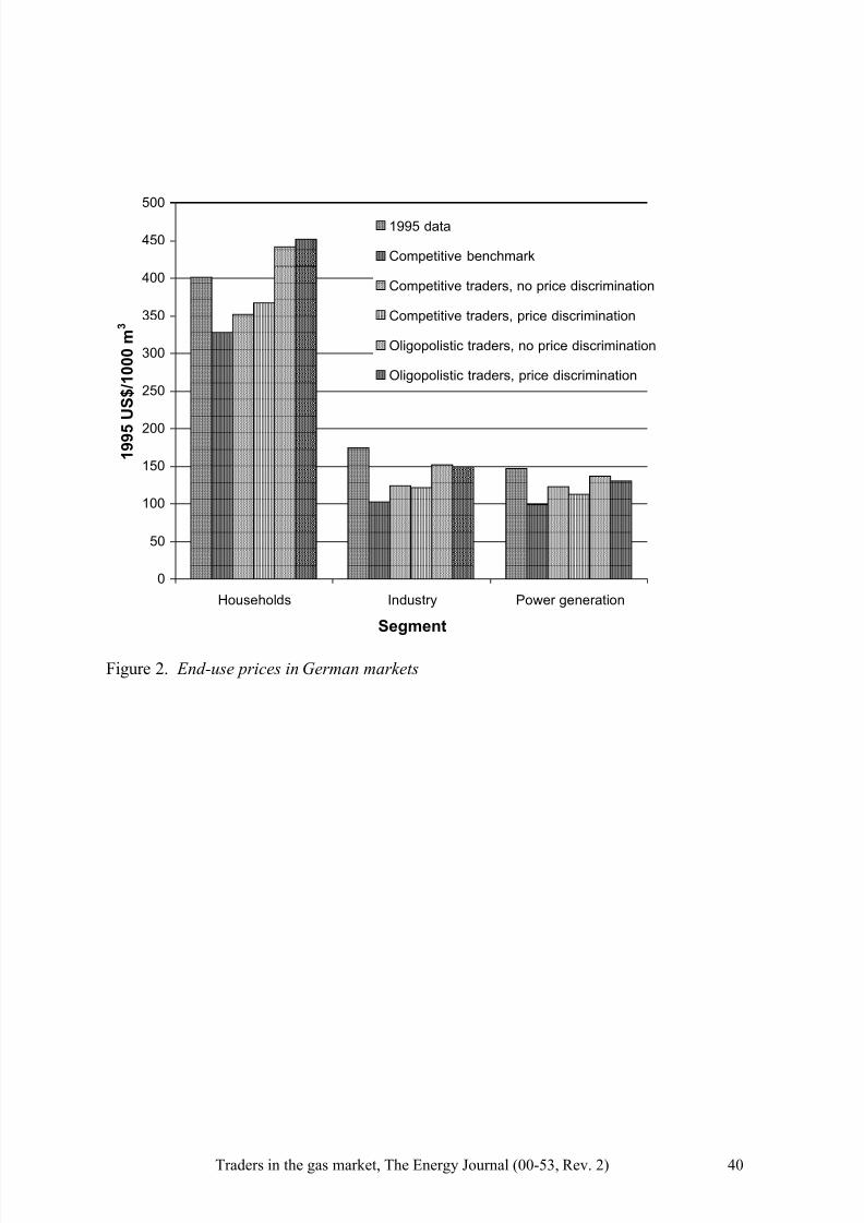
7/31/2019 10.1.1.199.6016



0

50

100

150

200

250

300

350

400

450

500

Households Industry Power generation

Segment

1 9 9 5

U S $ / 1 0 0 0 m

3

1995 data

Competitive benchmark

Competitive traders, no price discrimination

Competitive traders, price discrimination

Oligopolistic traders, no price discrimination

Oligopolistic traders, price discrimination

Figure 2. End-use prices in German markets

7/31/2019 10.1.1.199.6016


0

10000

20000

30000

40000

50000

60000

S u r p l u s Consumer surplus

Trader profit

Producer profit

Competitive BenchmarkOligopolistic Producers,

Competitive Traders

Oligopolistic Producers

& Traders

No border price

discrimination Border price discrimination

by producers

Figure 3. Total social welfare and its allocation among consumers, traders, and producers

10.1.1.199.6016

Documents