10.3 Time Series Thus FarWhereas cross sectional data needed 3

assumptions to make OLS unbiased, time series data needs only 2

-Although the third assumption is much stronger

-If we omit a valid variable, we cause biased as seen and calculated in Chapter 3

-Now all that remains is to derive assumptions that allow us to test the significance of our OLS estimates

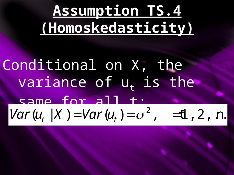
Assumption TS.4(Homoskedasticity)

Conditional on X, the variance of ut is the same for all t:

n.1,2,..., t,)()|( 2 tt uVarXuVar

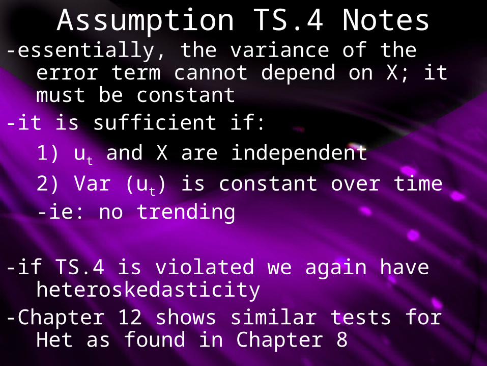
Assumption TS.4 Notes-essentially, the variance of the error term

cannot depend on X; it must be constant-it is sufficient if:

1) ut and X are independent

2) Var (ut) is constant over time-ie: no trending

-if TS.4 is violated we again have heteroskedasticity

-Chapter 12 shows similar tests for Het as found in Chapter 8

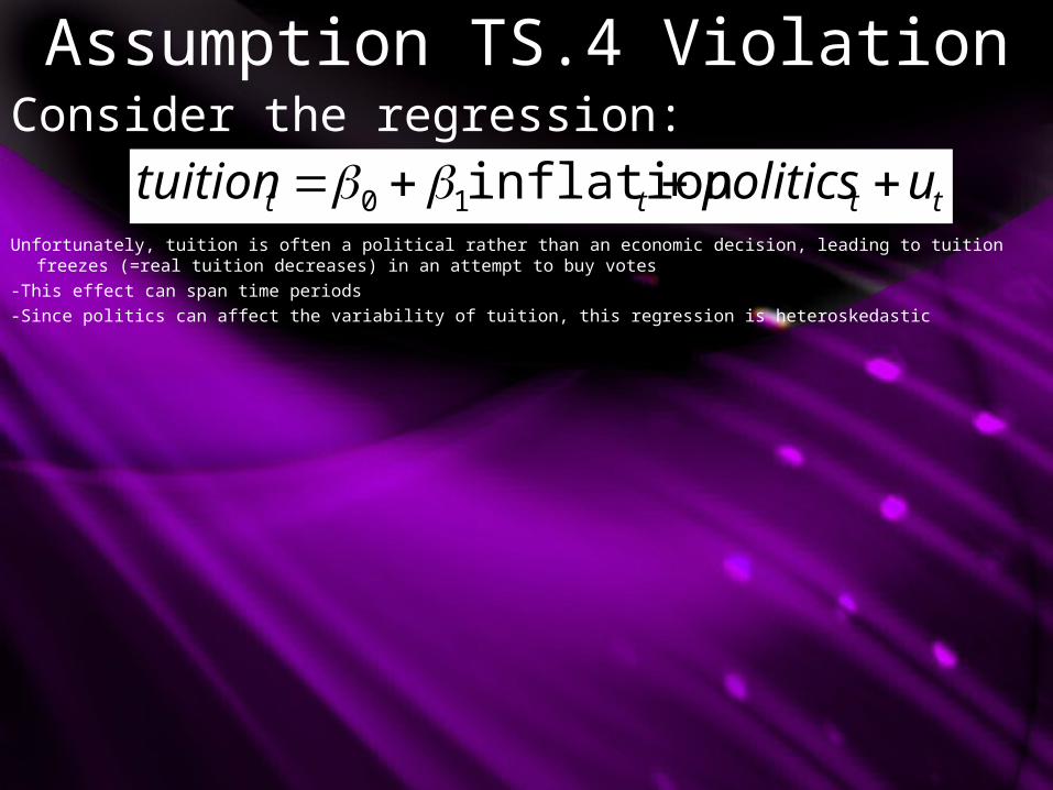
Assumption TS.4 ViolationConsider the regression:

tttt upoliticstuition inflation10 Unfortunately, tuition is often a political rather than an economic decision, leading to tuition freezes (=real

tuition decreases) in an attempt to buy votes-This effect can span time periods-Since politics can affect the variability of tuition, this regression is heteroskedastic

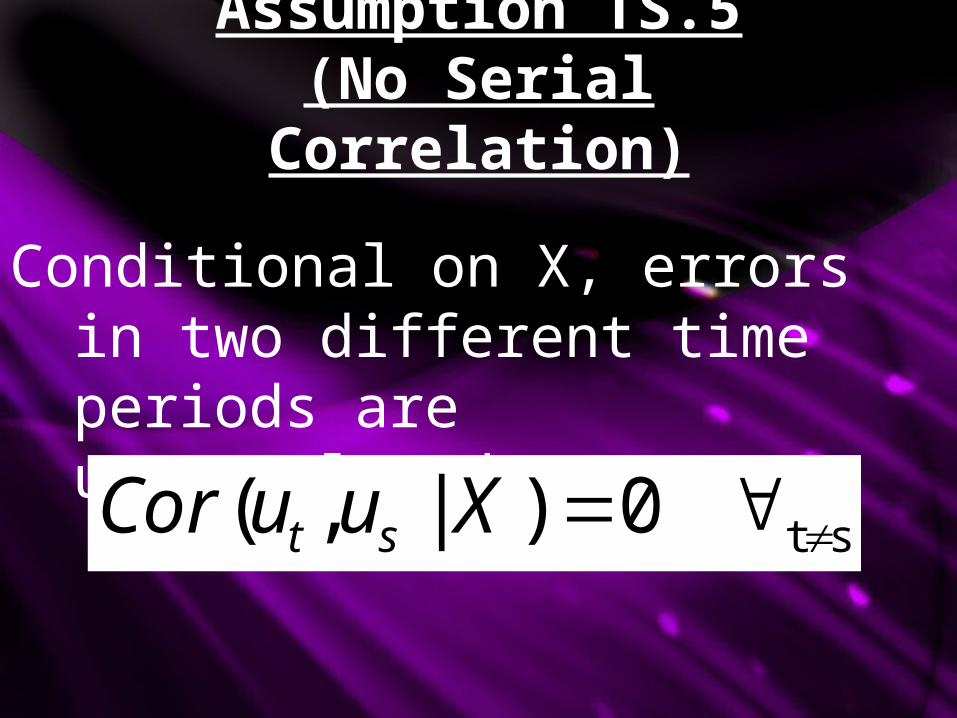
Assumption TS.5(No Serial Correlation)

Conditional on X, errors in two different time periods are uncorrelated:

st 0)|,( XuuCor st

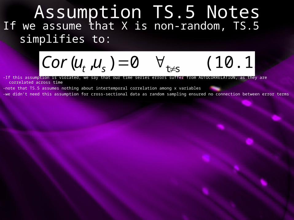
Assumption TS.5 NotesIf we assume that X is non-random, TS.5 simplifies

to:

(10.12) 0),( stst uuCor-If this assumption is violated, we say that our time series errors suffer from AUTOCORRELATION, as they are correlated

across time-note that TS.5 assumes nothing about intertemporal correlation among x variables-we didn’t need this assumption for cross-sectional data as random sampling ensured no connection between error terms

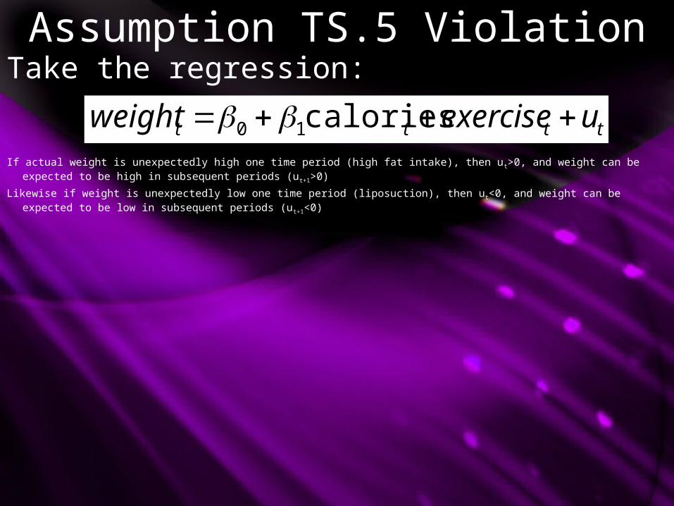
Assumption TS.5 ViolationTake the regression:

tttt uexerciseweight calories10 If actual weight is unexpectedly high one time period (high fat intake), then ut>0, and weight can be expected to be

high in subsequent periods (ut+1>0)

Likewise if weight is unexpectedly low one time period (liposuction), then ut<0, and weight can be expected to be low in subsequent periods (ut+1<0)

10.3 Gauss Markov Assumptions-Assumptions TS.1 through TS. 5 are our Gauss-Markov assumptions for time series data

-They allow us to estimate OLS variance-If cross sectional data is not random, TS.1 through TS.5 can sometimes be used in cross sectional applications-with these 5 properties in time series data, we see variance calculated and the Gauss-Markov theorem holding the same as with cross sectional data-the same OLS properties apply in finite sample time series as in cross-sectional data:

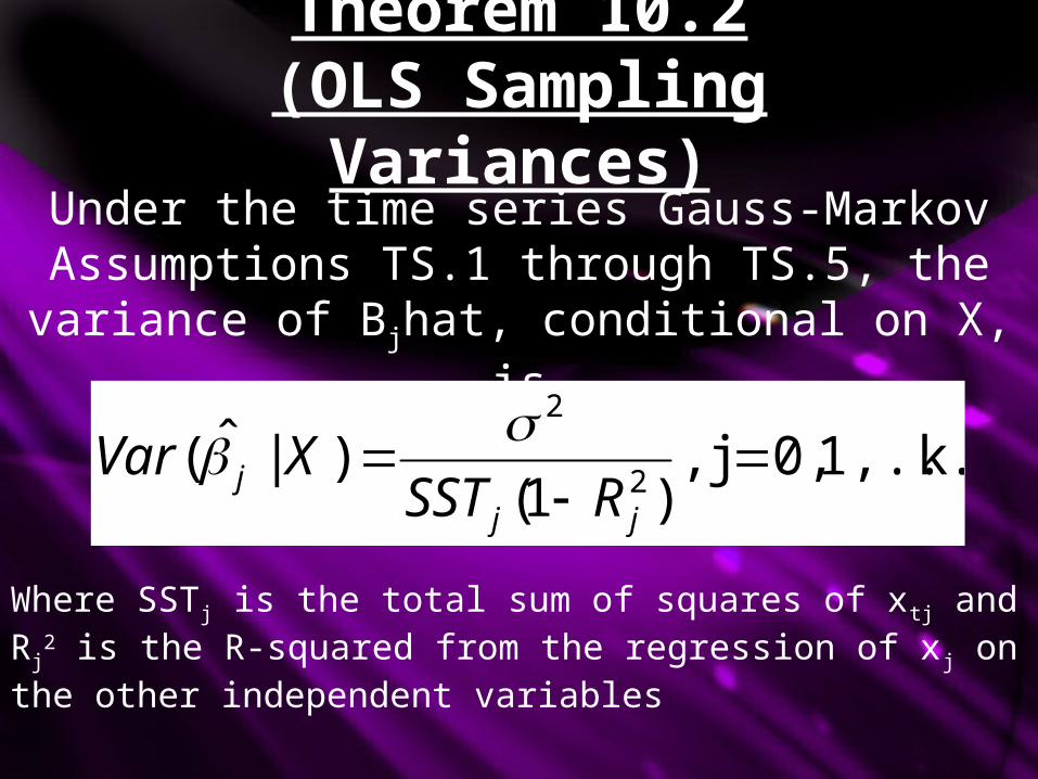
Theorem 10.2(OLS Sampling

Variances)Under the time series Gauss-Markov Assumptions TS.1 through TS.5, the variance of Bjhat, conditional on X, is

k.1,..., 0,j ,)1(

)|ˆ(2

2

jj

j RSSTXVar

Where SSTj is the total sum of squares of xtj and Rj2 is

the R-squared from the regression of xj on the other independent variables

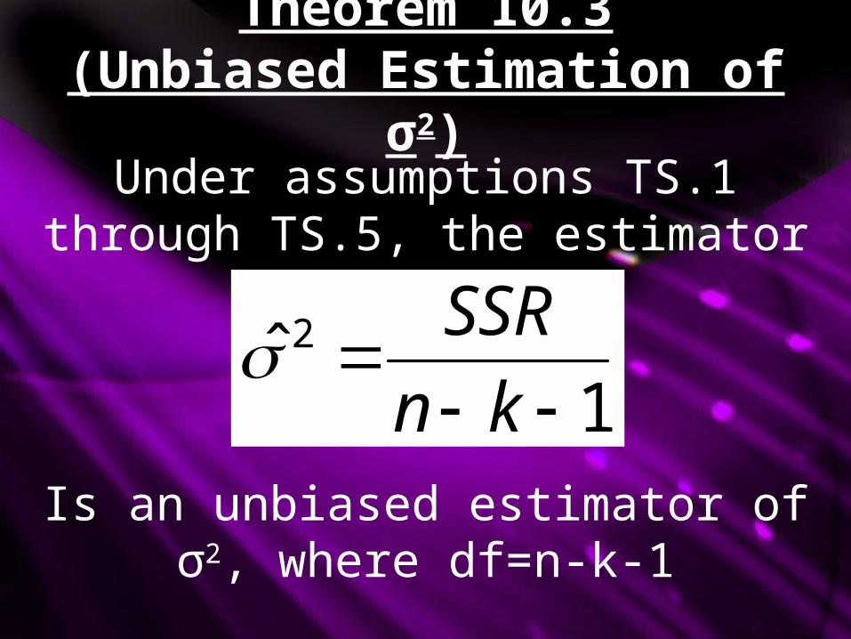
Theorem 10.3(Unbiased Estimation of

σ2)Under assumptions TS.1 through

TS.5, the estimator

1ˆ 2

kn

SSR

Is an unbiased estimator of σ2, where df=n-k-1

Theorem 10.4(Gauss-Markov

Theorem)

Under assumptions TS.1 through TS.5, the OLS

estimators are the best linear unbiased estimators

conditional on X

10.3 Time Series and Testing-In order to construct valid standard errors, t statistics and F statistics, we need to add one more assumption-TS.6 implies and is stronger than TS.3, TS.4 and TS.5-given these 6 time series assumptions, tests are conducted identically to the cross sectional case-time series assumptions are more restrictive than cross sectional assumptions

Assumption TS.6(Normality)

The errors ut are independent of X and are independently and identically distributed as Normal (0, σ2).

Theorem 10.5(Normal Sampling

Distribution)Under assumptions TS.1 through TS.6, the CLM assumptions for time series, the OLS estimators are normally distributed, conditional on X. Further, under the null hypothesis, each t statistic has a t distribution, and each F statistic has an F distribution. The usual construction of confidence intervals is also valid.

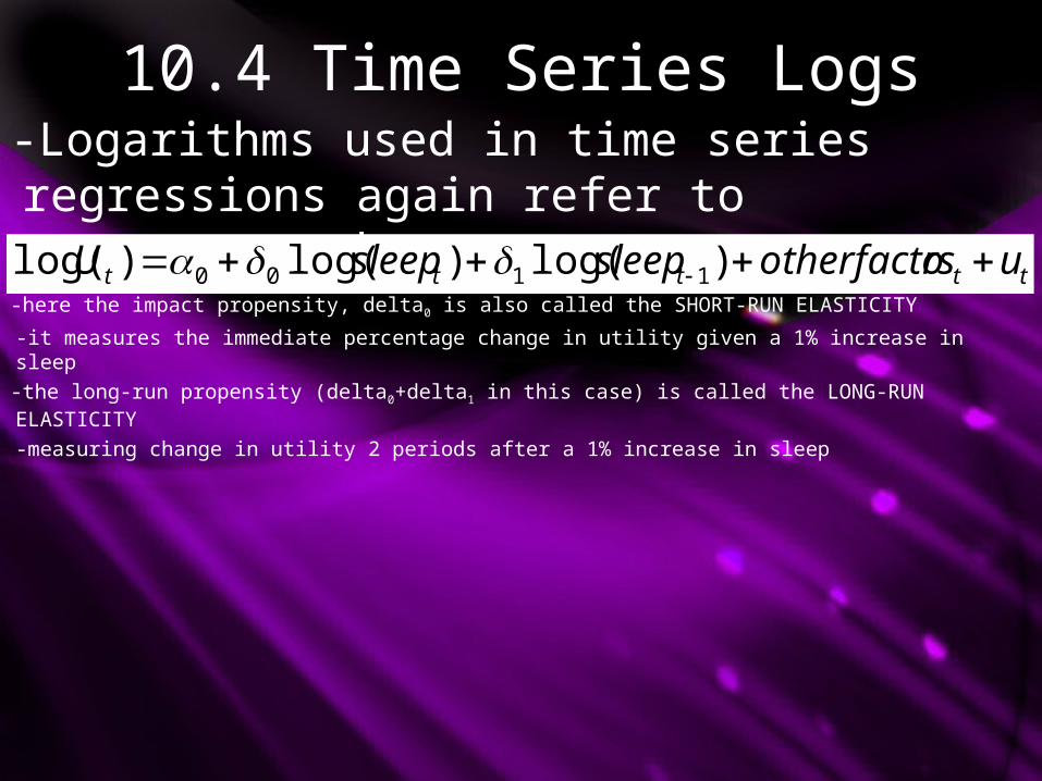
10.4 Time Series Logs-Logarithms used in time series regressions again refer to percentage changes:

ttttt ursotherfactosleepsleepU )log()log()log( 1100 -here the impact propensity, delta0 is also called the SHORT-RUN ELASTICITY

-it measures the immediate percentage change in utility given a 1% increase in sleep-the long-run propensity (delta0+delta1 in this case) is called the LONG-RUN ELASTICITY-measuring change in utility 2 periods after a 1% increase in sleep

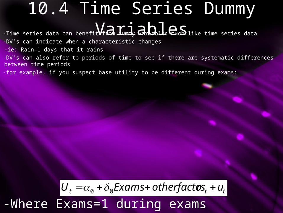
10.4 Time Series Dummy Variables-Time series data can benefit from dummy variables much like time series data

-DV’s can indicate when a characteristic changes-ie: Rain=1 days that it rains

-DV’s can also refer to periods of time to see if there are systematic differences between time periods-for example, if you suspect base utility to be different during exams:

ttt ursotherfactoExamsU 00 -Where Exams=1 during exams

10.4 Index Review-an index number aggregates a vast amount of information into a single quantity-for example, Econ 399 time can be spent in class, reviewing the text/notes, studying, working on assignments, or working on your paper

-since all these individual factors are highly correlated (an one hour in one area is not necessarily the same as one hour elsewhere) and numerous to conclude, work on Econ 399 can instead be shown as an index

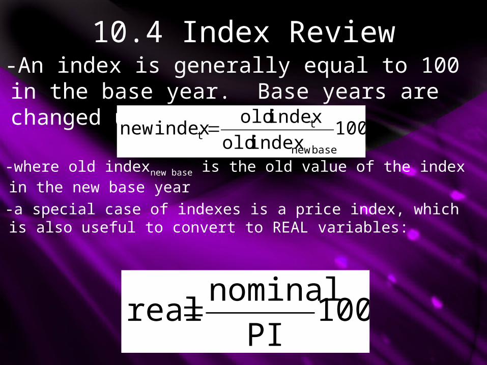
10.4 Index Review-An index is generally equal to 100 in the base year. Base years are changed using:

100index old

index oldindex new

base new

tt

-where old indexnew base is the old value of the index in the new base year-a special case of indexes is a price index, which is also useful to convert to REAL variables:

100PI

nominalreal

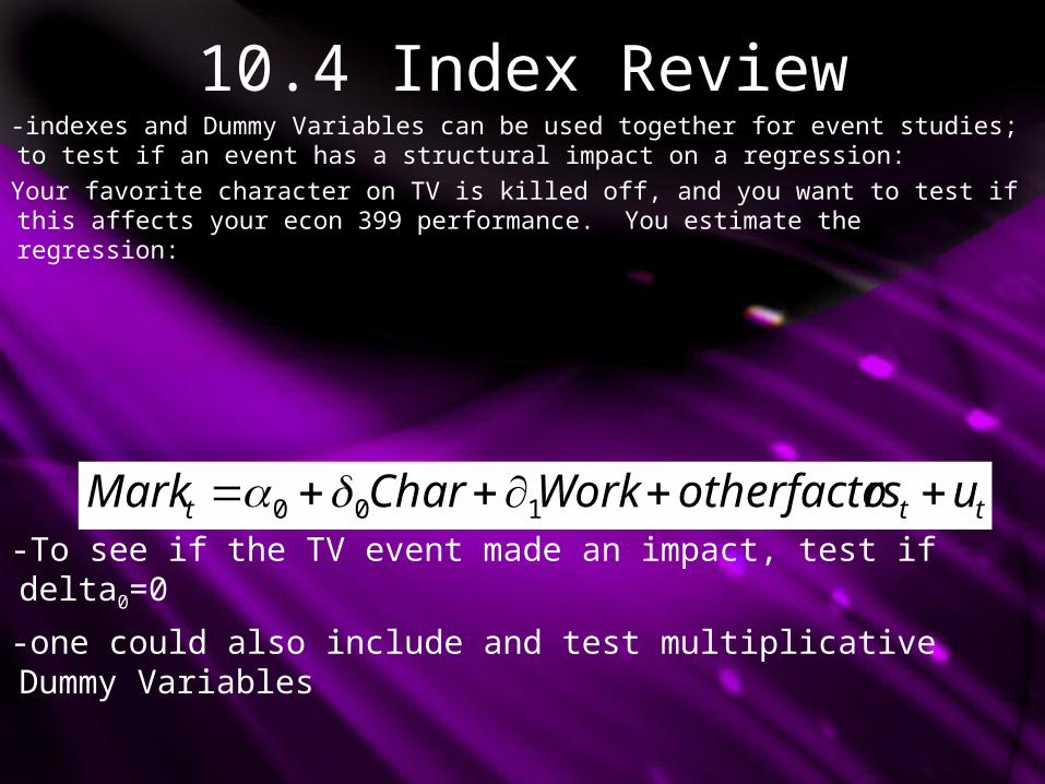
10.4 Index Review-indexes and Dummy Variables can be used together for event studies; to test if an event has a structural impact on a regression:Your favorite character on TV is killed off, and you want to test if this affects your econ 399 performance. You estimate the regression:

ttt ursotherfactoWorkCharMark 100 -To see if the TV event made an impact, test if delta0=0

-one could also include and test multiplicative Dummy Variables

10.5 Time Trends-Sometimes economic data has a TIME TREND; a tendency to grow over time-if two variables are either increasing or decreasing over time, they will appear to be correlated although they may be independent-failure to account for trending can lead to errors in a regression-even one variable trending in a regression can lead to errors, as we shall see

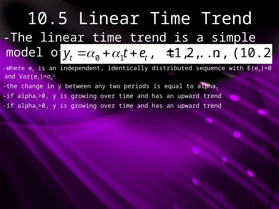
10.5 Linear Time Trend-The linear time trend is a simple model of trending: (10.24)n ..., 2, 1, t,10 tt ety

-Where et is an independent, identically distributed sequence with E(et)=0 and Var(et)=σe

2

-the change in y between any two periods is equal to alpha1

-if alpha1>0, y is growing over time and has an upward trend

-if alpha1>0, y is growing over time and has an upward trend

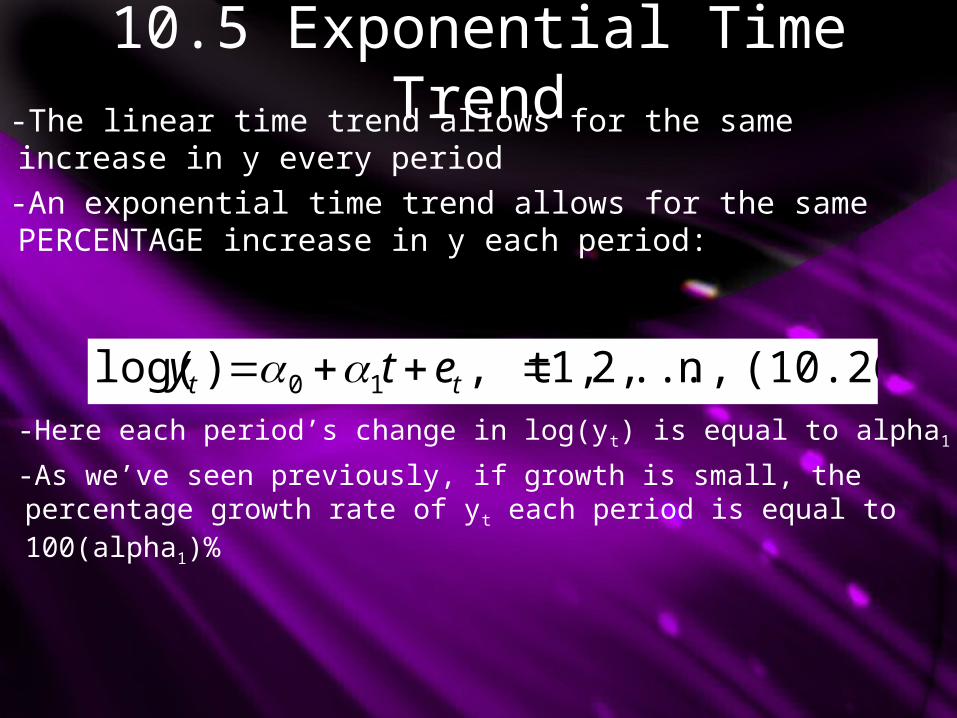
10.5 Exponential Time Trend-The linear time trend allows for the same increase in y every period-An exponential time trend allows for the same PERCENTAGE increase in y each period:

(10.26)n ..., 2, 1, t,)log( 10 tt ety -Here each period’s change in log(yt) is equal to alpha1

-As we’ve seen previously, if growth is small, the percentage growth rate of yt each period is equal to 100(alpha1)%

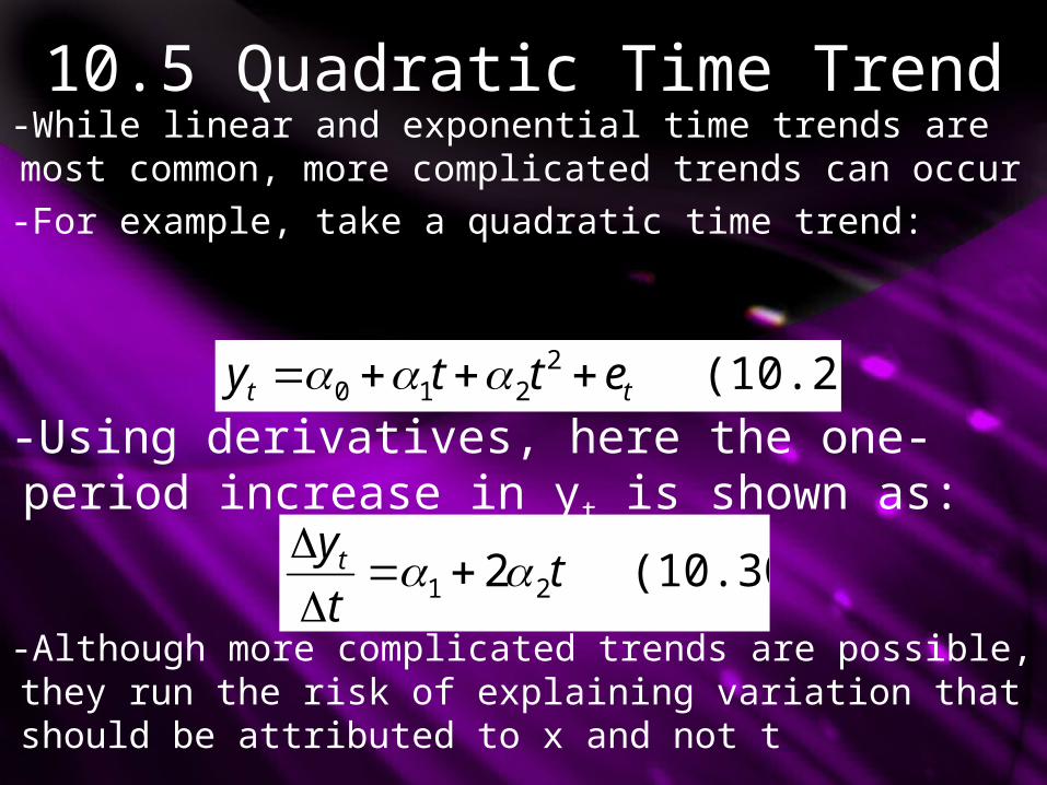
10.5 Quadratic Time Trend-While linear and exponential time trends are most common, more complicated trends can occur-For example, take a quadratic time trend:

(10.29) 2210 tt etty

-Using derivatives, here the one-period increase in yt is shown as:

(10.30) 2 21 tt

yt

-Although more complicated trends are possible, they run the risk of explaining variation that should be attributed to x and not t

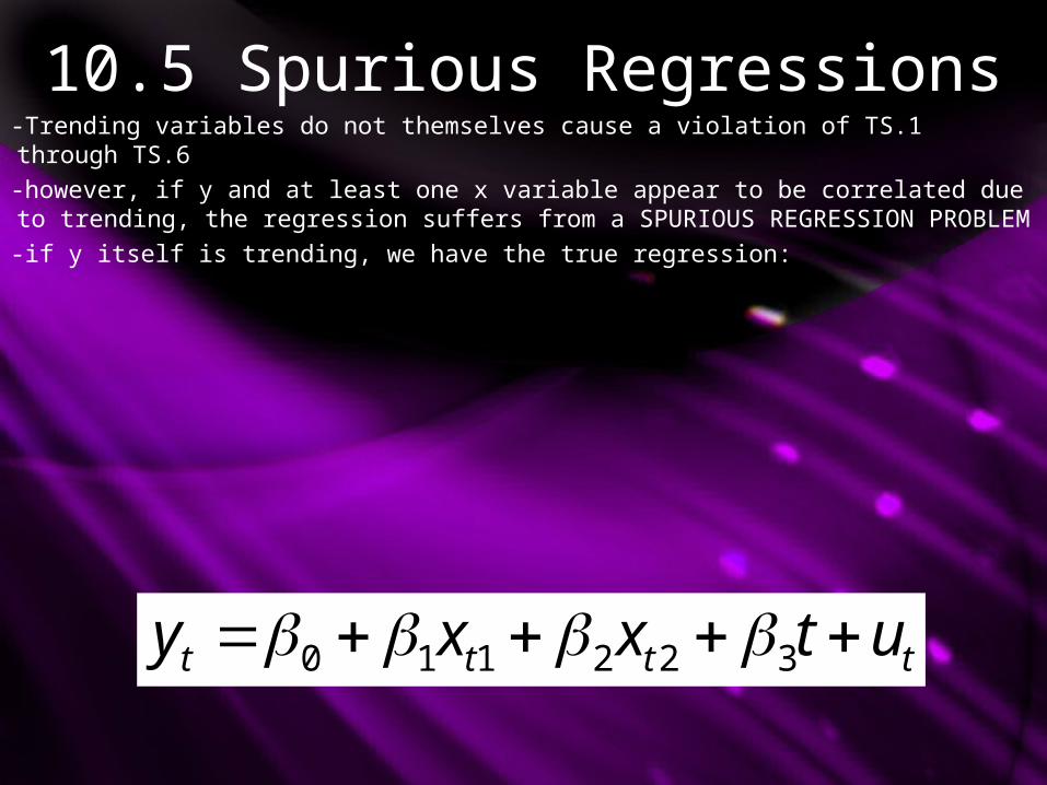
10.5 Spurious Regressions-Trending variables do not themselves cause a violation of TS.1 through TS.6

-however, if y and at least one x variable appear to be correlated due to trending, the regression suffers from a SPURIOUS REGRESSION PROBLEM

-if y itself is trending, we have the true regression:

tttt utxxy 322110

10.5 Spurious Regressions

tttt utxxy 322110 -If we omit the valid “variable” t, we have caused bias-this effect is heightened if x variables are also trending-adding a time trend can actually make a variable more significant if its movement about its trend affects y-note that including a time trend is also valid if only x (and not y) is trending

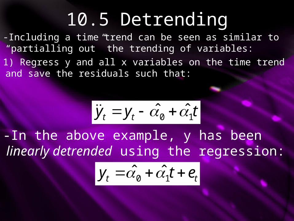
10.5 Detrending-Including a time trend can be seen as similar to “partialling out” the trending of variables:1) Regress y and all x variables on the time trend and save the residuals such that:

tyy tt 10 ˆˆ

-In the above example, y has been linearly detrended using the regression:

tt ety 10 ˆˆ

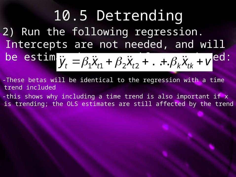
10.5 Detrending2) Run the following regression. Intercepts are not needed, and will be estimated as zero if not omitted: vxxxy tkkttt ...2211

-These betas will be identical to the regression with a time trend included-this shows why including a time trend is also important if x is trending; the OLS estimates are still affected by the trend

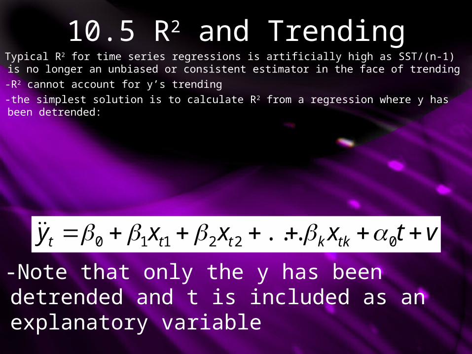
10.5 R2 and TrendingTypical R2 for time series regressions is artificially high as SST/(n-1) is no longer an unbiased or consistent estimator in the face of trending-R2 cannot account for y’s trending-the simplest solution is to calculate R2 from a regression where y has been detrended:

vtxxxy tkkttt 022110 ...

-Note that only the y has been detrended and t is included as an explanatory variable

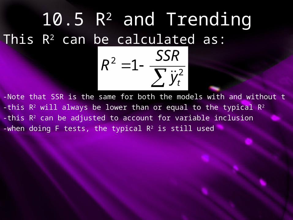
10.5 R2 and TrendingThis R2 can be calculated as:

22 1

ty

SSRR

-Note that SSR is the same for both the models with and without t-this R2 will always be lower than or equal to the typical R2

-this R2 can be adjusted to account for variable inclusion-when doing F tests, the typical R2 is still used

10.5 Seasonality-Some data may exhibit SEASONALITY, it may naturally vary within the year; within seasons-ie: housing starts, ice cream sales-typically data that exhibits seasonal patterns is seasonally adjusted-if this is not the case, seasonal dummy variables should be included (11 montly dummy variables, 3 seasonal dummy variables, etc)-significance tests can then be performed to evaluate the seasonality of the data

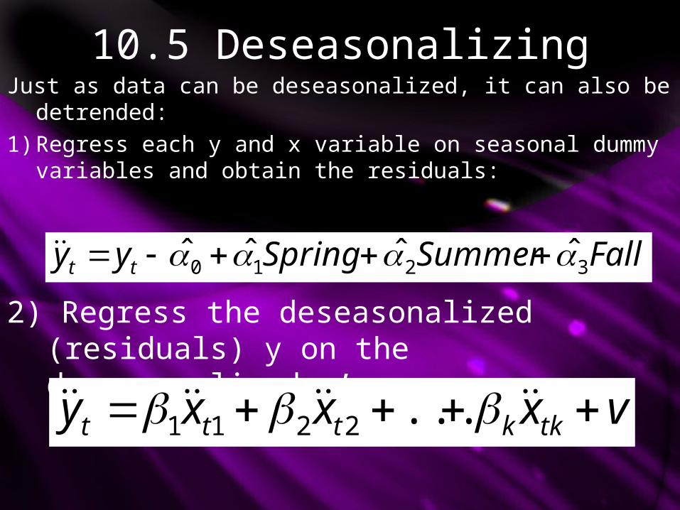
10.5 DeseasonalizingJust as data can be deseasonalized, it can also be

detrended:1) Regress each y and x variable on seasonal dummy

variables and obtain the residuals:

FallSummerSpringyy tt 3210 ˆˆˆˆ

2) Regress the deseasonalized (residuals) y on the deseasonalized x’s:

vxxxy tkkttt ...2211

10.5 DeseasonalizingThis deseasonalized model is again a better source for accurate R2 values

-as this model nets out any variation attributed to seasonality

-Note that some regressions may suffer from both trending and seasonality, requiring both detrending and deseasonalizing, which requires including seasonal dummy variables and a time trend in step 1 above.