1.1 introductionrandall-romero.com/wp-content/uploads/macro2-2018b/scarth-2014... · 1 keynes and...

1Keynes and the Classics

1.1 Introduction

Over 70 years have elapsed since the publication of Keynes’s The General Theory of Employment, Interest and Money (1936), yet the controversies between his followers and those macroeconomists who favour a more Classical approach have remained active. One purpose of this book is to examine some of these controversies, to draw attention to developments that have led to a synthesis of important ideas from both traditions, and to illustrate in some detail how this integrated approach can inform policy debates.

At the policy level, the hallmarks of Keynesian analysis are that involun-tary unemployment can exist and that, without government assistance, any adjustment of the system back to the ‘natural’ unemployment rate is likely to be slow and to involve cycles and overshoots. In its extreme form, the Keynesian view is that adjustment back to equilibrium simply does not take place without policy assistance. This view can be defended by maintaining either of the following positions: (1) the economy has multiple equilibria, only one of which involves ‘full’ employment; or (2) there is only one equi-librium, and it involves ‘full’ employment, but the economic system is unsta-ble without the assistance of policy, so it cannot reach the ‘full’ employment equilibrium on its own.

We shall consider the issue of multiple equilibria in Chapter 9. In earlier chapters, we focus on the question of convergence to a full equilibrium. To simplify the exposition, we concentrate on stability versus outright instabil-ity, which is the extreme form of the issue. We interpret any tendency toward outright instability as analytical support for the more general proposition that adjustment between full equilibria is protracted.

In this first chapter, we examine alternative specifications of the labour market, such as perfectly flexible money wages (the textbook Classical model) and completely fixed money wages (the textbook Keynesian model),

2 · Macroeconomics

to clarify some of the causes of unemployment. We consider fixed goods prices as well (the model of generalized disequilibrium), and then we build on this background in later chapters. For example, in Chapter 2, we assume that nominal rigidities are only temporary, and we consider a dynamic analysis that has Classical properties in full equilibrium, but Keynesian features in the transitional periods on the way to full equilibrium. Almost 60 years ago, Paul Samuelson (1955) labelled this class of dynamic models the Neoclassical Synthesis. This synthesis remained the core of mainstream macroeconomics until the 1970s, when practitioners became increasingly dissatisfied with two dimensions of this work: the limited treatment of expectations and the incomplete formal micro- foundations. We devote the next two chapters to addressing these shortcomings.

In Chapter 3, we explore alternative ways of bringing expectations into the analysis. One of the interesting insights to emerge is that, even with the Classicals’ most preferred specification for expectations, there is significant support for Keynes’s prediction that an increased degree of price flexibil-ity can increase the amount of cyclical unemployment that follows from a decrease in aggregate demand. In Chapter 4, we address the other major limitation of the analysis to that point – that formal micro- foundations have been missing. The inter- temporal optimization that is needed to overcome this shortcoming is explained in Chapter 4. Then, in Chapter 5, we examine the New Classical approach to business cycle analysis – the modern, more micro- based version of the market- clearing approach to macroeconomics, in which no appeal to sticky prices is involved. Then, in Chapters 6 and 7, we examine what has been called the ‘New’ Neoclassical Synthesis – a business cycle analysis that blends the microeconomic rigour of the New Classicals with the empirical applicability and a focus on certain market failures that have always been central features of the Keynesian tradition and the original Neoclassical Synthesis.

In the final five chapters of the book, the focus shifts from short- run stabiliza-tion issues to concerns about long- run living standards. In these chapters, we focus on structural unemployment and the challenge of raising productivity growth.

For the remainder of this introductory section, we discuss the two broad criteria economists have relied on when evaluating macro models. First, models are subjected to empirical tests, to see whether the predictions are consistent with actual experience. This criterion is fundamentally important. Unfortunately, however, it cannot be the only one for model selection, since empirical tests are often not definitive. Thus, while progress has been made

Keynes and the Classics · 3

in developing applied methods, macroeconomists have no choice but to put at least some weight on a second criterion for model evaluation.

Since the hypothesis of constrained maximization is at the core of our dis-cipline, all modern macroeconomists agree that macro models should be evaluated as to their consistency with optimizing underpinnings. Without a microeconomic base, there is no well- defined basis for arguing that either an ongoing stabilization policy or an increase in the average growth rate improves welfare. Increasingly, Keynesians have realized that they must acknowledge this point. Further, the challenge posed by New Classicals has forced Keynesians to admit that it is utility and production functions that are independent of government policy; agents’ decision rules do not neces-sarily remain invariant to shifts in policy. A specific microeconomic base is required to derive how private decision rules may be adjusted in the face of major changes in policy. Another advantage is that a specific microeconomic rationale imposes more structure on macro models, so the corresponding empirical work involves fewer ‘free’ parameters (parameters that are not constrained by theoretical considerations and can thus take on whatever value will maximize the fit of the model). It must be admitted that the empir-ical success of a model is compromised if the estimation involves many free parameters.

Despite these clear advantages of an explicit microeconomic base, those who typically stress these points – the New Classicals – have had to make some acknowledgements too. They have had to admit that, until recently, their models have been inconsistent with several important empirical regularities. As a result, many of them, like Keynesians, now allow for some temporary stickiness in nominal variables. Also, since the primary goal of this school of thought is to eliminate arbitrary assumptions, its followers should not down-play the significance of aggregation issues or of the non- uniqueness problem that often plagues the solution of their models. These issues have yet to be resolved in a satisfactory manner.

During the 1970s and 1980s, controversy between New Classicals and Keynesians was frustrating for students. Each group focused on the advan-tages of its own approach, and tended to ignore the legitimate criticisms offered by the ‘other side’. The discipline was fragmented into two schools of thought that did not interact. In the 1990s, however, there began an increased willingness on the part of macroeconomists to combine the best features of the competing approaches so that now the subject is empirically applicable, has solid micro- foundations, and allows for market failure – so economic policy can finally be explored in a rigorous fashion. Students can

4 · Macroeconomics

now explore models that combine the rigour of the New Classicals with the policy concern that preoccupies Keynesians.

The purpose of any model is to provide answers to a series of if–then ques-tions: if one assumes a specified change in the values of the exogenous vari-ables (those determined outside of the model), what will happen to the set of endogenous variables (those determined within the model)? A high degree of simultaneity seems to exist among the main endogenous variables (for example, household behaviour makes consumption depend on income, while the goods market- clearing condition makes output (and therefore income) depend on consumption). To cope with this simultaneity, we define macro models in the form of systems of equations for which standard solution tech-niques (either algebraic or geometric) can be employed. A model comprises a set of structural equations, which are definitions, equilibrium conditions, or behavioural reaction functions assumed on behalf of agents. The textbook Classical model, the textbook Keynesian model, the ‘more Keynesian’ model of generalized disequilibrium and the ‘new’ Classical model (all summarized graphically in later sections of this chapter) are standard examples.

In constructing these models, macroeconomists have disciplined their selec-tion of alternative behavioural rules by appealing to microeconomic models of households and firms. In other words, their basis for choosing structural equations is constrained maximization at the individual level, without much concern for problems of aggregation. To keep the analysis manageable, macroeconomists sometimes restrict attention to particular components of the macroeconomy, considered one at a time. They record the result-ing decision rules (the consumption function, the investment function, the money- demand function, the Phillips curve and so on, which are the first- order conditions of the constrained maximizations) as a list of structural equations. This series of equations is then brought together for solving as a standard set of simultaneous equations in which the unknowns are the endogenous variables. In other words, the procedure has two stages:

zz Stage 1: Derive the structural equations, which define the macro model, by presenting a set of (sometimes unconnected) constrained maxi-mization exercises (that is, define and solve a set of microeconomic problems).

zz Stage 2: Use the set of structural equations to derive the solution or reduced- form equations (in which each endogenous variable is related explicitly to nothing but exogenous variables and parameters) and perform the counterfactual exercises (for example, derivation of the policy multipliers).


Before 1970, macroeconomics developed in a fairly orderly way, follow-ing this two- stage approach. In recent decades, however, the discipline has seen some changes in basic approaches following from the fact that macro-economists have tried to consider ever more consistent and complicated theories of household and firm behaviour. That is, the specification of the constrained maximizations in stage 1 of the analysis has been made more general by allowing for such things as dynamics and the fact that agents must make decisions on the basis of expectations of the future.

This expansion has led to some conceptual and methodological complica-tions. Many analysts now regard it as unappealing to derive any one com-ponent structural equation without reference at stage 1 to the properties of the overall system. For example, if agents’ behaviour turns out to depend on expected inflation, it is tempting to model their forecast of inflation so that it is consistent with the actual inflation process, which is determined as one of the endogenous variables within the model. From a technical point of view, such an approach means that stages 1 and 2 must be considered simultane-ously. It also means that the form of at least some of the structural equations, and therefore the overall structure of the model itself, depends on the assumed time paths of the exogenous variables. Thus, it may be a bad practice for economists to use an estimated model found suitable for one data period as a mechanism for predicting what would happen in another period under a dif-ferent set of policy reactions. We shall consider this problem, which is referred to as the Lucas critique, in later chapters. Initially, however, we restrict atten-tion to models whose structures are assumed to be independent of the behav-iour of the exogenous variables. The textbook Keynesian and Classical models (covered in the remainder of this chapter) are examples of such models.

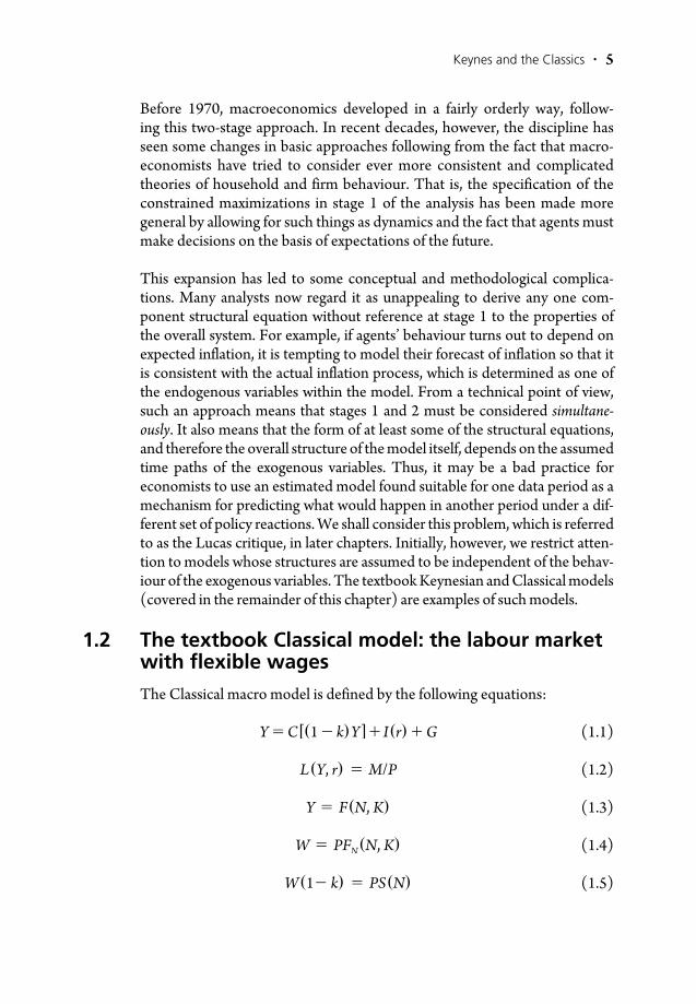
1.2 The textbook Classical model: the labour market with flexible wages

The Classical macro model is defined by the following equations:

Y 5 C [(1 2 k)Y ]1I(r) 1 G (1.1)

L (Y, r) 5 M/P (1.2)

Y 5 F (N, K) (1.3)

W 5 PFN (N, K) (1.4)

W (12 k) 5 PS(N) (1.5)

6 · Macroeconomics

Equations 1.1 and 1.2 are the IS and LM relationships; the symbols Y, C, I, G, M, P, k and r denote real output, household consumption, firms’ investment spending, government program spending, the nominal money supply, the price of goods, the proportional income tax rate and the interest rate. Since we ignore expectations at this point, anticipated inflation is assumed to be zero, so there is no difference between the nominal and real interest rates. The standard assumptions concerning the behavioural equations (with partial derivatives indicated by subscripts) are: Ir, Ir , 0, LY . 0, 0 , k, CYd , 1. The usual specification of government policy (that G, k and M are set exogenously) is also imposed. The aggregate demand for goods relation-ship follows from the IS and LM functions, as is explained below.

Equations 1.3, 1.4 and 1.5 are the production, labour demand and labour supply functions, where W, N and K stand for the nominal wage rate, the level of employment of labour and the capital stock. The assumptions we make about the production function are standard (that is, the marginal prod-ucts are positive and diminishing): FN, FK, FNK 5 FKN . 0, FNN, FKK , 0. Equation 1.4 involves the assumption of profit maximization: firms hire workers up to the point that labour’s marginal product equals the real wage. It is assumed that it is not optimal for firms to follow a similar optimal hiring rule for capital, since there are installation costs. The details of this con-straint are explained in Chapter 4; here we simply follow convention and assume that firms invest more in new capital, the lower are borrowing costs. We allow for a positively sloped labour supply curve by assuming SN . 0. Workers care about the after- tax real wage, W(1 − k)/P.

In the present system, the five equations determine five endogenous vari-ables: Y, N, r, P and W. However, the system is not fully simultaneous. Equations 1.4 and 1.5 form a subset that can determine employment and the real wage w 5 W/P. If the real wage is eliminated by substitution, equations 1.4 and 1.5 become FN (N, K) 5 S(N)/(1 2 k) . Since k and K are given exog-enously, N is determined by this one equation, which is the labour market equilibrium condition. This equilibrium value of employment can then be substituted into the production function, equation 1.3, to determine output. Thus, this model involves what is called the Classical dichotomy: the key real variables (output and employment) are determined solely on the basis of aggregate supply relationships (the factor market relations and the produc-tion function), while the demand considerations (the IS and LM curves) determine the other variables (r and P) residually.

The model can be pictured in terms of aggregate demand and supply curves (in price- output space), so the term ‘supply- side economics’ can be appre-


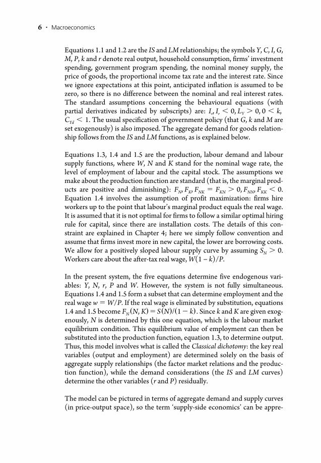
ciated. The aggregate demand curve comes from equations 1.1 and 1.2. Figure 1.1 gives the graphic derivation. The aggregate demand curve in the lower panel represents all those combinations of price and output that satisfy the demands for goods and assets. To check that this aggregate demand curve is negatively sloped, we take the total differential of the IS and LM equations, set the exogenous variable changes to zero, and solve for(dP/dY) after eliminating (dr) by substitution. The result is:

Slope of the aggregate demand curve 5 (rise/run in P- Y space):

dP/dY 5 2 [LY Lr1 Lr (1 2 CYd (1 2 k))] /[Ir M/P2 ] , 0 (1.6)

The aggregate supply curve is vertical, since P does not even enter the equa-tion (any value of P, along with the labour market- clearing level of Y, satisfies these supply conditions). The summary picture, with shift variables listed in parentheses after the label for each curve, is shown in Figure 1.2. The key policy implication is that the standard monetary and fiscal policy variables, G and M, involve price effects only. For example, complete ‘crowding out’ follows increases in government spending (that is, output is not affected). The reason is that higher prices shrink the real value of the money supply so that interest rates are pushed up and pre- existing private investment

r

P

D

ISY

Y

LM

P2

P2

P1

P1

P0

P0

Figure 1.1 Derivation of the aggregate demand curve

8 · Macroeconomics

expenditures are reduced. Nevertheless, tax policy has a role to play in this model. A tax cut shifts both the supply and the demand curves to the right. Thus, output and employment must increase, although price may go up or down. Blinder (1973) formally derives the (dP/dk) multiplier and, consider-ing plausible parameter values, argues that it is negative. ‘Supply- side’ econo-mists are those who favour applying this ‘textbook Classical model’ to actual policy making (as was done in the United States in the 1980s, when the more specific label ‘Reaganomics’ was used).

From a graphic point of view, the ‘Classical dichotomy’ feature of this model follows from the fact that it has a vertical aggregate supply curve. But the position of this vertical line can be shifted by tax policy. A policy of balanced- budget reduction in the size of government makes some macroeconomic sense here. Cuts in G and k may largely cancel each other in terms of affect-ing the position of the demand curve, but the lower tax rate stimulates labour supply, and so shifts the aggregate supply curve for goods to the right. Workers are willing to offer their services at a lower before- tax wage rate, so profit- maximizing firms are willing to hire more workers. Thus, according to this model, both higher output and lower prices can follow tax cuts.

This model also suggests that significantly reduced prices can be assured (without reduced output rates) if the money supply is reduced. Such a policy shifts the aggregate demand curve to the left but does not move the vertical aggregate supply curve. In the early 1980s, several Western countries tried a policy package of tax cuts along with decreased money supply growth; the motive for this policy package was, to a large extent, the belief that the Classical macro model has some short- run policy relevance. Such policies are controversial, however, because a number of analysts believe that the model ignores some key questions. Is the real- world supply curve approximately vertical in the short run? Are labour supply elasticities large enough to lead to a significant shift in aggregate supply? A number of economists doubt that these conditions are satisfied. Another key issue is the effect on macro-

D(M,G,k)Y

P S(K,k)Figure 1.2 Aggregate demand and supply curves


economic performance that the growing government debt that accompanies this combination policy might have. After all, a decreased reliance on both taxation and money issue as methods of government finance, at the same time, may trap the government into an ever- increasing debt problem. The textbook Classical model abstracts from this consideration (as do the other standard models that we review in this introductory chapter). An explicit treatment of government debt is considered later in this book (in Chapter 7). At this point we simply report that a negative verdict on the possibility of tax cuts paying for themselves has emerged (in addition, see Mankiw and Weinzierl, 2006).

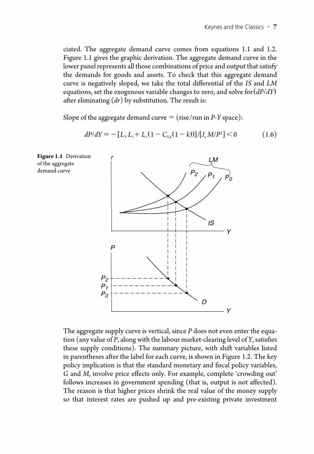
Before leaving the textbook Classical model, we summarize a graphic exposi-tion that highlights both the goods market and the labour market. In Figure 1.3, consider that the economy starts at point A. Then a decrease in government spending occurs. The initial effect is a leftward shift of the IS curve (and therefore in the aggregate demand curve). At the initial price level, aggregate

Y

Y

Y Y

W

Production function

N

N

P

A

B

A

B P · FN

(1 – k)P · S(N)

45°

Labour market

D

S

Aggregate supply anddemand

Y–

N–

Figure 1.3 The Classical model

10 · Macroeconomics

supply exceeds aggregate demand. The result is a fall in the price level, and this (in turn) causes two shifts in the labour market quadrant of Figure 1.3: (1) labour demand shifts down (because of the decrease in the marginal revenue product of labour); and (2) labour supply shifts down by the same proportion-ate amount as the decrease in the price level (because of workers’ decreased money- wage claims). Both workers and firms care about real wages; had we drawn the labour market with the real wage on the vertical axis, neither the first nor the second shift would occur. These shifts occur because we must ‘correct’ for having drawn the labour demand and supply curves with refer-ence to the nominal wage. The final observation point for the economy is B in both bottom panels of Figure 1.3. The economy avoids ever having a reces-sion in actual output and employment, since the shock is fully absorbed by the falling wages and prices. These fixed levels of output and employment are often referred as the economy’s ‘natural rates’ (denoted here by Y and N ).

Many economists find this model unappealing; they think they do observe recessions in response to drops in aggregate demand. Indeed, many have interpreted both the 1930s and the recent recession in 2008 as having been caused by drops in demand. What changes are required in the Classical model to make the system consistent with the existence of recessions and unemployment? We consider the New Classicals’ response to this question in section 1.5 of this chapter. But, before that, we focus on the traditional Keynesian responses. Keynes considered: (1) money- wage rigidity; (2) a model of generalized disequilibrium involving both money- wage and price rigidity; and (3) expectations effects that could destabilize the economy. The first and second points can be discussed in a static framework and so are analysed in the next section of this introductory chapter. The third point requires a dynamic analysis, which will be undertaken in Chapters 2 and 3.

1.3 The textbook Keynesian model: the labour market with money- wage rigidity

Contracts, explicit or implicit, often fix money wages for a period of time. In Chapter 8, we shall consider some of the considerations that might moti-vate these contracts. For the present, however, we simply presume the exist-ence of fixed money- wage contracts and we explore their macroeconomic implications.

On the assumption that money wages are fixed by contracts for the entire relevant short run, W is now taken as an exogenous variable stuck at value W. Some further change in the model is required, however, since otherwise we would now have five equations in four unknowns – Y, N, r and P.


Since the money wage does not clear the labour market in this case, we must distinguish actual employment, labour demand and labour supply, which are all equal only in equilibrium. The standard assumption in disequilibrium analyses is to assume that firms have the ‘right to manage’ the size of their labour force during the period after which the wage has been set. This means that labour demand is always satisfied, and that the five endogenous vari-ables are nowY, r, P, N, NS, where the latter variable is desired labour supply. Since this variable occurs nowhere in the model except in equation 1.5, that equation solves residually for NS. Actual employment is determined by the intersection of the labour demand curve and the given money- wage line.

Figure 1.4 is a graphic representation of the results of a decrease in govern-ment spending. As before, we start from the observation point A and assume a decrease in government spending that moves the aggregate demand curve to the left. The resulting excess supply of goods causes price to decrease, with the same shifts in the labour demand and the labour supply curves as were discussed above. The observation point becomes B in both panels of Figure 1.4. The unemployment rate, which was zero, is now BD/CD. Unemployment has two components: lay- offs, AB, plus increased participa-tion in the labour force, AD.

The short- run aggregate supply curve in the Keynesian model is positively sloped, and this is why the model does not display the Classical dichotomy results (that is, why demand shocks have real effects). The reader can verify that the aggregate supply curve’s slope is positive, by taking the total dif-ferential of the key equations (1.3 and 1.4) while imposing the assumptions

A DB

N

C

W P

Y

B

A

S

D

N–

Y–

W—

P · FN

P · S(N)(1 – k)

Figure 1.4 Fixed money wages and excess labour supply


that wages and the capital stock are fixed in the short run (that is, by settingdW 5 dK 5 0). After eliminating the change in employment by substitu-tion, the result is the expression for the slope of the aggregate supply curve:

dP/dY 5 2PFNN/F 2N . 0. (1.7)

The entire position of this short- run aggregate supply curve is shifted up and in to the left if there is an increase in the wage rate (in symbols, an increase in W). A similar change in any input price has the same effect. Thus, for an oil- using economy, an increase in the price of oil causes stagflation – a simul-taneous increase in both unemployment and inflation.

Additional considerations can be modelled on the demand side of the labour market as well. For example, if we assume that there is monopolistic competi-tion, the marginal- cost- equals- marginal- revenue condition becomes slightly more complicated. Marginal cost still equals W/FN, but marginal revenue becomes equal to [1 2 1/(ne)]P where n and e are the number of firms in the industry (economy) and the elasticity of the demand curve for the industry’s (whole economy’s) output. In this case, the number of firms becomes a shift influence for the position of the demand curve for labour. If the number of firms rises in good times and falls in bad times, the corresponding shifts in the position of the labour demand curve (and therefore in the position of the goods supply curve) generate a series of booms and recessions. And real wages will rise during the booms and fall during the recessions (that is, the real wage will move pro- cyclically). But this imperfect- competition exten-sion of the standard textbook Keynesian model is rarely considered. As a result, the following summary is what has become conventional wisdom.

Unemployment occurs in the Keynesian model because of wage rigidity. This can be reduced by any of the following policies: increasing government spending, increasing the money supply or reducing the money wage (think of an exogenous decrease in wages accomplished by policy as the static equivalent of a wage guidelines policy). These policy propositions can be proved by verifying that dN/dG, dN/dM . 0 and that dN/dW , 0. Using more everyday language, the properties of the perfect- competition version of the rigid money- wage model are:

1. Unemployment can exist only because the wage is ‘too high’.2. Unemployment can be lowered only if the level of real incomes of those

already employed (the real wage) is reduced.3. The level of the real wage must correlate inversely with the level of

employment (that is, it must move contra- cyclically).


Intermediate textbooks call this model the Keynesian system. However, many economists who regard themselves as Keynesians have a difficult time accepting these three propositions. They know that Keynes argued, in Chapter 19 of The General Theory, that large wage cuts might have only worsened the Depression of the 1930s. They feel that unemployment stems from some kind of market failure, so it should be possible to help unem-ployed workers without hurting those already employed. Finally, they have observed that there is no strong contra- cyclical movement to the real wage; indeed, it often increases slightly when employment increases (see Solon et al., 1994 and Huang et al., 2004).

1.4 Generalized disequilibrium: money- wage and price rigidity

These inconsistencies between Keynesian beliefs on the one hand and the properties of the textbook (perfect competition version of the) Keynesian model on the other suggest that Keynesian economists must have developed other models that involve more fundamental departures from the Classical system. One of these developments is the generalization of the notion of disequilibrium to apply beyond the labour market, a concept pioneered by Barro and Grossman (1971) and Malinvaud (1977).

If the price level is rigid in the short run, the aggregate supply curve is hor-izontal. There are two ways in which this specification can be defended. One becomes evident when we focus on slope expression (equation 1.7). This expression equals zero if FNN 5 0. To put the point verbally, the mar-ginal product of labour is constant if labour and capital must be combined in fixed proportions. This set of assumptions – rigid money wages and fixed- coefficient technology – is often appealed to in defending fixed- price models. (Note that these models are the opposite of supply- side economics, since, with a horizontal supply curve, output is completely demand- determined, not supply- determined.)

Another defence for price rigidity is simply the existence of long- term con-tracts fixing the money price of goods as well as the money price of factors. To use this interpretation, however, we must re- derive the equations in the macro model that relate to firms, since, if the goods market is not clearing, it may no longer be sensible for firms to set marginal revenue equal to marginal cost. This situation is evident in Figure 1.5, which shows a perfectly com-petitive firm facing a sales constraint. If there were no sales constraint, the firm would operate at point A, with marginal revenue (which equals price) equal to marginal cost. Since marginal cost 5 W (dN/dY)5 W/FN, this is the


assumption we have made throughout our analysis of Keynesian models up to this point. But, if the market price is fixed for a time (at P) and aggregate demand falls so that all firms face a sales constraint (sales fixed at Y|), the firm will operate at point B. The marginal revenue schedule now has two compo-nents: PB and Y|D in Figure 1.5. Thus, marginal revenue and marginal cost diverge by amount BC.

We derive formally the factor demand equations in Chapter 4 – both those relevant for the textbook Classical and textbook Keynesian models (where there is no sales constraint), and those relevant for this generalized disequi-librium version of Keynesian economics. Here, we simply assert the results that are obtained in the sticky- goods- price case. First, the labour demand curve becomes a vertical line (in wage- employment space). The correspond-ing equation is simply the production function – inverted and solved for N – which stipulates that labour demand is whatever solves the produc-tion function after the historically determined value for the capital stock and the sales- constrained value for output have been substituted in. The revised investment function follows immediately from cost minimization. Firms should invest more in capital whenever the excess of capital’s marginal product over labour’s marginal product is bigger than the excess of capital’s rental price over labour’s rental price. Using d to denote capital’s deprecia-tion rate, the investment function that is derived in Chapter 4 is:

I 5 a [ (FK (W/P) ) / (FN (r 1 d) ) 2 1 ] . (1.8)

The model now has two key differences from what we labelled the text-book Keynesian model. First, labour demand is now independent of the real wage, so any reduction in the real wage does not help in raising employment. Second, the real wage is now a shift variable for the IS curve, and therefore for the aggregate demand curve for goods, so nominal wage cuts can decrease

Pricemarginal cost

Sales constraint

Output

Marginal cost

AB

C

D

P–

Y~

Figure 1.5 A competitive firm facing a sales constraint


aggregate demand and thereby lower employment. (This second point is explained more fully below.) These properties can be verified formally by noting that the model becomes simply equations 1.1 to 1.3 but with W and P exogenous and with the revised investment function replacing I(r). The three endogenous variables are Y, r and N, with N solved residually by equation 1.3.

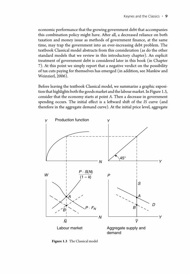
The model is presented graphically in Figure 1.6. The initial observation point is A in both the goods and labour markets. Assume a decrease in gov-ernment expenditure. The demand for goods curve moves left so firms can only sell Y|; the labour demand curve becomes the N| line, and the observa-tion point moves to point B in both diagrams. Unemployment clearly exists. Can it be eliminated? Increases in M or G would shift the demand for goods back, so these policies would still work. But what about a wage cut? If the W line shifts down, all that happens is that income is redistributed from labour to capitalists (as shown by the shaded rectangle). If capitalists have a smaller marginal propensity to consume than workers, the demand for goods shifts further to the left, leading to further declines in real output and employment. The demand for goods shifts to the left in any event, however, since, given the modified investment function (equation 1.8), the lower wage reduces investment. Thus, wage cuts actually make unemployment worse.

Some Keynesians find this generalized disequilibrium model appealing, since it supports the proposition that activist aggregate demand policy can still successfully cure recessions while wage cuts cannot. Thus the unemployed can be helped without taking from workers who are already employed (that is, without having to lower the real wage). However, the prediction that wage

Y

D

P

AB

W

N

ABW—

N~

N—

P—

P · FN

P · S(N)

(1 – k)

Y~

Y~

Y–

Figure 1.6 The effects of falling demand with fixed wages and prices


cuts lead to lower employment requires the assumption that prices do not fall as wages do. In Figure 1.6, the reader can verify that, if both the given wage and price lines shift down (so that the real wage remains constant), output and employment must increase. The falling price allows point B to shift down the dashed aggregate demand curve for goods, so the sales- constrained level of output rises (sales become less constrained). Further, with a less binding sales constraint, the position of the vertical labour demand curve shifts to the right.

Many economists are not comfortable with the assumption that goods prices are more sticky than money wages. This discomfort forces them to downplay the significance of the prediction that wage cuts could worsen a recession, at least as shown in generalized disequilibrium models of the sort just summa-rized. As a result, other implications of sticky prices are sometimes stressed. One concerns the accumulation of inventories that must occur when firms are surprised by an emerging sales constraint. In the standard models, firms simply accept this build- up and never attempt to work inventories back down to some target level. Macro models focusing on inventory fluctuations were very popular many years ago (for example, Metzler, 1941). Space limitations preclude our reviewing these analyses, but the reader is encouraged to consult Blinder (1981). Suffice it to say here that macroeconomic stability is prob-lematic when firms try to work off large inventory holdings, since periods of excess supply must be followed by periods of excess demand. As a result, it is difficult to avoid overshoots when inventories are explicitly modelled. Readers wishing to pursue the disequilibrium literature more generally should consult Stoneman (1979) and especially Backhouse and Boianovsky (2013).

It may have occurred to readers that more Keynesian results would emerge from this analysis if the aggregate demand curve were not negatively sloped. For example, if it were vertical, a falling goods price would never remove the initial sales constraint. And, if the demand curve were positively sloped, falling prices would make the sales constraint ever more binding. Is there any reason to believe that such non- standard versions of the aggregate demand curve warrant serious consideration? Keynes would have answered ‘yes’, since he stressed a phenomenon which he called a ‘liquidity trap’. This special case of our general model can be considered by letting the interest sensitiv-ity of money demand become very large: Lr S 2`. By checking the slope expression for the aggregate demand curve (equation 1.6 above), the reader can verify that this situation involves the aggregate demand curve becom-ing ever steeper and becoming vertical. In this case, falling wages and prices cannot eliminate the recession. And this situation can be expected to emerge if interest rates become so low that expected capital losses on assets other


than money are deemed a certainty. This is precisely what Keynes thought was relevant in the 1930s, and what others have thought was relevant in Japan in the 1990s and in the United States after the 2008 recession – all periods when the short- term nominal interest rate became zero.

More Classically minded economists have always dismissed the relevance of the liquidity trap, since they have noted that the vertical- demand- curve feature does not emerge when the textbook model is extended in a simple way. Following Pigou (1943), they have allowed the household consumption–savings decision to depend on the quantity of liquid assets available, not just on the level of disposable income – by making the consumption function C[(1 − k)Y, M/P]. With this second term in the consumption function, known as the Pigou effect, the aggregate demand curve remains negatively sloped, since falling prices raise the real value of household money hold-ings and so they stimulate spending directly, even if there is a liquidity trap. However, according to Tobin’s (1975) interpretation, the Pigou effect has been paid far too much attention. Tobin prefers to stress I. Fisher’s (1933) debt- deflation analysis. Tobin notes that the nation’s money supply is mostly people’s deposits in banks, and that almost all of these deposits are matched on the banks’ balance sheets by other people’s loans. A falling price of goods raises both the real value of lenders’ assets and the real value of borrowers’ liabilities. The overall effect on aggregate demand depends on the propensi-ties to consume of the two groups. Given that borrowers take out loans to spend, they must have higher spending propensities than lenders. Indeed, people who can afford to be lenders are thought to operate according to the permanent income hypothesis, adjusting their saving to insulate their current consumption from cyclical outcomes. So Fisher stressed that the effect of falling prices on borrowers would have to be the dominant consideration. With their debts rising in real terms as prices fall, they have to reduce their spending. Overall, then, the aggregate demand curve is positively sloped in periods when the liquidity trap is relevant.

We can use this insight to provide a simplified explanation of recent work by Farmer (2010, 2013a, 2013b). Farmer argues against the disequilibrium tra-dition in Keynesian analysis, since he thinks that sticky wages and prices are not the essence of Keynes at all. Farmer believes that the Classical demand for explicit micro- foundations must be respected, but he advocates a version of those foundations that can lead to multiple equilibria. In this approach, the essence of Keynes is that an exogenous change in ‘confidence’ can shift the economy from one equilibrium to another, and no appeal to sticky prices or irrationality is needed to defend how this outcome can emerge. Farmer generates the multiple- equilibria feature from a particular search- theoretic


interpretation of the labour market (which we explain in Chapters 8 and 9). But we can illustrate the essence of his approach more simply by appealing to Solow’s (1979) simplest version of efficiency- wage theory. As explained in Chapter 8, when worker productivity depends positively on the real wage workers receive, and when firms face a sales constraint, cost- minimizing firms find it in their interest to keep the real wage constant (even if the level of that sales constraint changes, and even if nominal wages and prices are falling).

We now combine this efficiency- wage theory of the labour market with Farmer’s suggestion that we take nominal GDP as exogenously depend-ing on people’s confidence (what Keynes referred to as ‘animal spirits’). In price- output space, the exogenous nominal GDP locus is a negatively sloped rectangular hyperbola. A drop in confidence shifts this locus toward the origin in the graph. If a positively sloped aggregate demand curve closes the model, the flexible- price equilibrium point shifts in the south- west direction: we observe falling prices and falling output. And people’s expectations are fulfilled, so there is no inconsistency with the initial assumption that caused the shift. Flexible wages and prices do not move the economy away from this new outcome point unless they reverse animal spirits, but there is no reason for this expectational effect to emerge – given the logical structure of the model. While this is a very simplified version of Farmer’s work, it is sufficient to make readers aware of the fact that there are important strands of Keynesian analysis that both reject the traditional Keynesian emphasis on disequilibrium and accept the modern dictum that macroeconomics involve explicit micro- foundations.

1.5 The New Classical model

Previous sections of this chapter have summarized the traditional macro models, the ones that are labelled Classical and Keynesian in intermediate- level texts. In recent decades, the term ‘new’ has been introduced to indicate that modern Classical and Keynesian macroeconomists have extended these traditional analyses. We examine this work in later chapters (Chapter 5 in the case of New Classicals and Chapter 8 in the case of New Keynesians). But it is useful to put these developments into a simple aggregate supply and demand context at this stage, and that is why we considered the work of both the generalized disequilibrium theorists and Farmer in the preceding section. The present section turns to a brief summary of the New Classical approach (again, in terms of basic aggregate supply and demand curves). As above, the goal at this stage is to allow readers to appreciate how the new work compares to the more traditional intermediate- level discussions.


New Classicals have extended the micro- foundations of their models to allow for inter- temporal decision making. One key dimension is the house-hold labour–leisure choice. When optimizing, individuals consider not just whether to work or take leisure now, but also whether to work now or in the future. This choice is made by comparing the current real wage with the expected present value of the future real wage. The value of the real interest rate affects this calculation: a higher interest rate lowers the discounted value of future work and so stimulates labour supply today. This means that the entire position of the present period’s labour supply curve, and therefore of the goods supply curve (which remains a vertical line, since wages and prices are still assumed to be fully flexible), depends on the interest rate. As a result, in the algebraic derivation of the current aggregate supply curve of goods, the IS relationship is used to eliminate the interest rate. The implication is that any of the standard shift influences for IS move the aggregate supply curve, not the aggregate demand curve, in this model. Actually, the standard IS rela-tionship is replaced by one that is developed from a dynamic optimization base, but that modification need not concern us at this stage.

Following the thought experiment that we have considered in earlier sec-tions of this chapter, consider a decrease in autonomous spending (G) as an example event that allows us to appreciate some of the properties of this New Classical framework. The first thing to consider is the effect on the interest rate and, for this, Classicals focus on the loanable funds market (with savings and investment as the supply and demand schedules respectively). Savings is output not consumed, so lower government spending on consumption goods increases national savings. With the supply curve for loanable funds shifting to the right, a lower interest rate emerges. With a higher discounted value for future work, households postpone supplying labour until this higher reward can be had, so they work less today. The result of this leftward shift in today’s labour supply function is lower employment, so in the goods market graph the vertical aggregate supply curve shifts to the left. Real GDP falls, and the real wage rises, just as these variables move – for different reasons – in the traditional Keynesian models.

With the IS relationship now a part of the supply side of the goods market, what lies behind the aggregate demand function in price- output space? The answer: the LM relationship. For illustration, let us consider the simplest version of that relationship – the monetarist special case in which the inter-est sensitivity of money demand is zero and the income elasticity is unity. This ‘quantity- theory’ special case implies that the transactions velocity of money, V, is a constant, so the equation of the aggregate demand curve is PY 5 MV. In price- output space, this is a rectangular hyperbola which shifts


closer or farther from the origin as MV falls or rises. The position of this locus is not affected by variations in autonomous spending. So the fall in G that we discussed in the previous paragraph moves the supply curve, not the demand curve, to the left. The New Classical model predicts the same as the Keynesian models do for output (a lower value for real output) but the opposite prediction for the price level (that price rises).

There are other differences in the models’ predictions. For example, the Keynesian models suggest that the reduction in employment can be inter-preted as lay- offs, so that the resulting unemployment can be thought of as involuntary. In the New Classical model, on the other hand, the reduction in employment must be interpreted as voluntary quits, since with continu-ous clearing in the labour market there is never any unemployment. Put another way, the Keynesian models predict variation in the unemployment rate, while the New Classical model predicts variation in the participation rate. But for the most basic Classical dichotomy question – can variations in the demand for goods cause variations in real economic activity – the New Classical model answers ‘yes’, and in this way it departs from the traditional Classical model. We pursue the New Classical research agenda more fully in Chapter 5.

1.6 Conclusions

In this chapter we have reviewed Keynesian and Classical interpretations of the goods and labour markets. Some economists, known as post- Keynesians, would argue that our analysis has been far too Classically focused, since they feel that what is traditionally called Keynesian – New or otherwise – misses much of the essence of Keynes. One post- Keynesian concern is that the traditional tools of aggregate supply and demand involve inherent logical inconsistencies. For a recent debate of these allegations, see Grieve (2010), Moseley (2010) and Scarth (2010a). Another post- Keynesian concern is that mainstream analysis treats uncertainty in a way that Keynes argued was silly. Keynes followed Knight’s (1921) suggestion that risk and uncertainty were fundamentally different. Risky outcomes can be dealt with by assuming a stable probability distribution of outcomes, but some events occur so infre-quently that the relevant actuarial information is not available. According to post- Keynesians, such truly uncertain outcomes simply cannot be mod-elled formally. Yet one more issue raised by post- Keynesians is that a truly central concept within mainstream macroeconomics – the aggregate pro-duction function – cannot be defended. We assess this allegation in Chapter 4, but beyond that we leave the concerns of the post- Keynesians to one side. Given our objective of providing a concise text that focuses on what is


usually highlighted in a one- semester course, we cannot afford to consider post- Keynesian analysis further in this book. Instead, we direct readers to Wolfson (1994), and focus on the New Classical and New Keynesian reviv-als, and the synthesis of these approaches that has emerged, in our later chapters.

Among other things, in this chapter we have established that – as long as we ignore New Keynesian developments that focus on market failures (such as asymmetric information that leads to the payment of real wages above market clearing levels) – unemployment can exist only in the presence of some stickiness in money wages. Appreciation of this fact naturally leads to a question: should we advocate increased wage and price flexibility? We proceed with further macroeconomic analysis of this and related questions in Chapter 2, while we postpone our investigation of the microeconomic models of sticky wages and prices, market failures and multiple equilibria until later chapters.

1.1 introductionrandall-romero.com/wp-content/uploads/macro2-2018b/scarth-2014... · 1 keynes and...

Documents