Complex critical points and curved geometries in four-dimensional Lorentzianspinfoam quantum gravity

Muxin Han,1, 2, ∗ Zichang Huang,3, 4, † Hongguang Liu,2, ‡ and Dongxue Qu1, §

1Department of Physics, Florida Atlantic University,777 Glades Road, Boca Raton, FL 33431-0991, USA

2Institut für Quantengravitation, Universität Erlangen-Nürnberg, Staudtstr. 7/B2, 91058 Erlangen, Germany3Department of Physics, Center for Field Theory and Particle Physics,

and Institute for Nano- electronic devices and Quantum computing, Fudan University, Shanghai 200433, China4State Key Laboratory of Surface Physics, Fudan University, Shanghai 200433, China

This paper focuses on the semiclassical behavior of the spinfoam quantum gravity in 4 dimensions.There has been long-standing confusion, known as the flatness problem, about whether the curvedgeometry exists in the semiclassical regime of the spinfoam amplitude. The confusion is resolvedby the present work. By numerical computations, we explicitly find curved Regge geometries fromthe large-j Lorentzian Engle-Pereira-Rovelli-Livine (EPRL) spinfoam amplitudes on triangulations.These curved geometries are with small deficit angles and relate to the complex critical points ofthe amplitude. The dominant contribution from the curved geometry to the spinfoam amplitude isproportional to eiI , where I is the Regge action of the geometry plus corrections of higher orderin curvature. As a result, the spinfoam amplitude reduces to an integral over Regge geometriesweighted by eiI in the semiclassical regime. As a byproduct, our result also provides a mechanism torelax the cosine problem in the spinfoam model. Our results provide important evidence supportingthe semiclassical consistency of the spinfoam quantum gravity.

The semiclassical consistency is an important require-ment in quantum physics. Any satisfactory quantumtheory must reproduce the corresponding classical theoryin the approximation of small ~. In particular, the role ofsemiclassical analysis is more crucial in the field of quan-tum gravity. Due to the limitation of experimental tests,the semiclassical consistency is one of only few physicalconstraints for quantum gravity: a satisfactory quantumtheory of gravity must reproduce General Relativity (GR)in the semiclassical regime.This paper focuses on the semiclassical analysis of

Loop Quantum Gravity (LQG). LQG as a background-independent and non-perturbative approach has beendemonstrated to be a competitive candidate toward thefinal quantum gravity theory (see e.g., [1–6] for reviews).The path integral formulation of LQG, known as thespinfoam theory [7–11], is particularly interesting for test-ing the semiclassical consistency of LQG, because of theconnection between the semiclassical approximation ofpath integral and the stationary phase approximation.A central object in the spinfoam theory is the spinfoamamplitude, which defines the covariant transition ampli-tude of LQG. The recent semiclassical analysis reveals theinteresting relation between spinfoam amplitudes and theRegge calculus, which discretizes GR on triangulations[12–19]. This relation makes the semiclassical consistencyof the spinfoam theory promising.

Nevertheless, it has been argued that an accidental flat-ness constraint might emerge in the semiclassical regime,

∗ hanm(AT)fau.edu† hzc881126(AT)hotmail.com‡ hongguang.liu(AT)gravity.fau.de§ dqu2017(AT)fau.edu

so that spinfoam amplitudes would be dominated by onlyflat Regge geometries, whereas curved geometries wereabsent [20–24]. The suspicion of lacking curved geometryin the semiclassical regime has lead to the doubt aboutthe semiclassical behavior. This flatness problem has beena key issue in the spinfoam LQG for more than a decade.In this work, we resolve the flatness problem by ex-

plicitly finding curved Regge geometries from the 4-dimensional Lorentzian EPRL spinfoam amplitude. Thesecurved geometries are with small deficit angles δh, andhave been overlooked in the model because they corre-spond to complex critical points slightly away from thereal integration domain. But they can be revealed bya more refined stationary phase analysis involving theanalytic continuation of the spinfoam integrand. Thesecurved Regge geometries still give non-suppressed domi-nant contributions to the spinfoam amplitude. The con-tributions are proportional to eiI where I is the Reggeaction of the curved geometry plus corrections of the sec-ond and higher orders in δh. The spinfoam amplitudereduces to an integral over Regge geometries weighted byeiI in the semiclassical regime.

These results are illustrated by the numerical analysisof the EPRL spinfoam amplitudes on triangulations ∆3

and σ1-5 (FIG.1(a) and (b)). As a byproduct, the “cosineproblem” [25] is shown to be relaxed on ∆3.

Our results provide important evidence supporting thesemiclassical consistency of the spinfoam theory.Spinfoam amplitude.—The 4-dimensional triangulationK contains 4-simplices v, tetrahedra e, triangles f , linesegments, and points. We denote the internal triangleby h and the boundary triangle by b (f is either h or b),and assign the SU(2) spins jh, jb ∈ N0/2 to internal andboundary triangles h, b. The spin jf = jh or jb relatesto the quantum area of f by af = 8πγG~

√jf (jf + 1)

arX

iv:2

110.

1067

0v1

[gr

-qc]

20

Oct

202

1

2

[26, 27]. The Lorentzian EPRL spinfoam amplitude on Ksums over internal spins jh:

A(K) =∑jh

∏h

djh

∫[dgdz] eS(jh,gve,zvf ;jb,ξeb), (1)

[dgdz] =∏(v,e)

dgve∏

(v,f)

dΩzvf, (2)

where djh = 2jh + 1. The spinfoam action S is com-plex and linear to jh, jb [15]. The boundary states ofA(K) are SU(2) coherent states |jb, ξeb〉 where ξeb =ueb (1, 0)T , ueb ∈ SU(2). jb, ξeb determines the areaand the 3-normal of b in the boundary tetrahedron e.The summed/integrated variables are gve ∈ SL(2,C),zvf ∈ CP1, and jh. The boundary jb, ξeb are notsummed/integrated. dgve is the SL(2,C) Haar measure.dΩzvf

is a scaling invariant measure on CP1. A cut-offjmaxh should be imposed if

∑jh

leads to divergence.By the area spectrum, the classical area af and small ~

imply the large spin jf 1. This motivates to understandthe large-j regime as the semiclassical regime of A(K).To probe the semiclassical regime, we scale uniformlyjb, jh → λjb, λjh, where λ 1. Scaling spins impliesS → λS. Moreover, it is convenient to apply the Poissonsummation formula to replace the sum over jh by integral

A(K) =∑kh∈Z

∫ ∏h

djh∏h

(2λdλjh)

∫[dgdz] eλS

(k)

, (3)

S(k) = S + 4πi∑h

jhkh, (4)

where jh is real and continuous.The details of A(K), S,and Poission summation are reviewed in Appendix I.Real critical points and flatness.—For each kh in (3),

by the stationary phase method, the integral with λ 1 is approximated by the dominant contributions fromsolutions of the critical equations

Re(S) = ∂gveS = ∂zvf

S = 0, (5)∂jhS = 4πikh, kh ∈ Z. (6)

The solution inside the integration domain is denoted byjh, gve, zvf. We view the integration domain as a realmanifold, and call jh, gve, zvf the real critical point.

Every solution satisfying the part (5) and a nondegen-eracy condition endows a Regge geometry to K with 4dorientation [12–15]. Further imposing (6) to these Reggegeometries gives the accidental flatness constraint to everydeficit angle δh hinged by the internal triangle h [22, 23]

γδh = 4πkh, kh ∈ Z. (7)

The Barbero-Immirzi parameter γ 6= 0 is finite. Whenkh = 0, δh at every internal triangle is zero, so the Reggegeometry endowed by the real critical point is flat. Ifthe dominant contribution to A(K) with λ 1 onlycomes from real critical points, Eq.(7) implies that onlythe flat geometry and geometries with γδh = ±4πZ+ can

𝒁(𝒓)

𝒙 = 𝒁(𝒓) Re(𝒛)

Im(𝒛)

(a)

(b) (c)

1

2

3 4

56

2

4 6

1

53

2

4

1

53

2

6

1

53

4 6

1

53

FIG. 1. (a) The ∆3 triangulation (the center panel) made bygluing three 4-simplices (in blue, red, and purple). The internaltriangle (135) is highlighted in red. (b) The triangulation σ1-5

made by the 1-5 Pachner move dividing a 4-simplex intofive 4-simplices. σ1-5 has 10 internal triangles and 5 internalsegments I = 1, · · · , 5 (red). (c) The real and complex criticalpoints x and Z(r). S(r, z) is analytic extended from the realaxis to the complex neighborhood illustrated by the red disk.

contribute dominantly to A(K), whereas the contributionsfrom generic curved geometries are suppressed. If thiswas true, the semiclassical behavior of A(K) would fail tobe consistent with GR.A generic jh, gve, zvf can endow discontinuous 4d

orientation, i.e., the orientation flips between 4-simplices.Then (7) becomes γ

∑v∈h svΘh(v) = 4πkh where sv = ±1

labels two possible orientations at each 4-simplex v. Θh(v)is the dihedral angle hinged by h in v.Complex critical points.—As we will show, the large-λ

spinfoam amplitude does receive non-suppressed contribu-tions from curved geometries with small but nonzero |δh|.Demonstrating this property needs a more refined station-ary phase analysis for the complex action with parameters[28, 29]: We consider the large-λ integral

∫KeλS(r,x)dNx,

and regard r as parameters. S(r, x) is an analytic functionof r ∈ U ⊂ Rk, x ∈ K ⊂ RN . U ×K is a neighborhoodof (r, x). x is a real critical point of S(r, x). S(r, z),z = x + iy ∈ CN , is the analytic extension of S(r, x)to a complex neighborhood of x. The complex criticalequation ∂zS = 0 is solved by z = Z(r) where Z(r) isan analytic function of r in the neighborhood U . Whenr = r, Z (r) = x reduces to the real critical point. Whenr deviates away from r, Z(r) ∈ CN can move away from

3

the real plane RN , thus is called the complex critical point(see FIG.1(b)). We have the following large-λ asymptoticexpansion for the integral∫

K

eλS(r,x)dNx =

(1

λ

)N2 eλS(r,Z(r))√

det(−δ2

z,zS(r, Z(r))/2π)

× [1 +O(1/λ)] (8)

where S(r, Z(r)) and δ2z,zS(r, Z(r)) are the action and

Hessian at the complex critical point.The crucial information of (8) is: the integral can re-

ceive the dominant contribution from the complex criticalpoint away from the real plane. This fact has been over-looked by the argument of the flatness problem.Asymptotics of A(∆3).—We firstly focus on a simpler

example A(∆3) where ∆3 contains three 4-simplices anda single internal triangle h. All line segments of ∆3 areat the boundary, and their lengths determine the Reggegeometry g on ∆3. So g is fixed by the (Regge-like)boundary data jb, ξeb that uniquely corresponds to theboundary segment-lengths.

Translate the general theory toward (8) to A(∆3): r =

jb, ξeb is the boundary data. r = jb, ξeb determinesthe flat geometry g(r) with δh = 0. x = jh, gve, zvfis the real critical point associated to r and endows theorientations sv = +1 to all 4-simplices. r, g(r), and xare computed numerically in Appendices IIA - II B. Theintegration domain of A(∆3) is 124 real dimensional. Wedefine local coordinates x ∈ R124 covering the neighbor-hood of x inside the integration domain (see AppendixII C). S(r, x) is the spinfoam action, analytic in the neigh-borhood of (r, x). z ∈ C124 complexifies x. S(r, z) extendsholomorphically S(r, x) to a complex neighborhood of x.We only complexify x but do not complexify r. We focuson kh = 0, since the integrals with kh 6= 0 have no realcritical point when r = r, and are suppressed even whentaking into account complex critical points, as far as δhis not close to 4πkh.We vary the length l26 of the line segment connect-

ing the points 2 and 6, leaving other segment lengthsunchanged. A family of (Regge-like) boundary datar = r + δr parametrized by l26 is obtained numerically,and gives the family of curved geometries g(r) with δh 6= 0(see Appendix IID).

At each r, the real critical point is absent. Butwe find the complex critical point z = Z(r) satisfying∂zS(r, z) = 0 with high-precision numerics. The detailsabout the numerical solution and error analysis are givenin Appendix II E. We insert Z(r) into S(r, z), and com-pute numerically the difference between S(r, Z(r)) andthe Regge action IR of the curved geometry g(r):

δI(r) = S(r, Z(r))− iIR[g(r)], (9)

where IR[g(r)] = ah(r)δh(r) +∑b

ab(r)Θb(r).(10)

The areas ah(r), ab(r) and deficit/dihedral angles

(a) (b)

(c)

(e)

1.5×10-12 1.5×10-8 0.00015δh

1.

0.9

0.8

0.7

0.6

0.5

eλRe[δℐ]

10-14 10-12 10-10 10-8 10-6 10-4δh

0.4

0.6

0.8

1.0eλRe[δℐ]

(d)

(f)

<latexit sha1_base64="+VKucry2xu1d47EVc67mAsjeu4o=">AAAB7XicbVBNS8NAEJ3Ur1q/qh69BIvgqSRS0WPRi8cK9gPaUDabTbt2sxt2J0Ip/Q9ePCji1f/jzX/jts1BWx8MPN6bYWZemApu0PO+ncLa+sbmVnG7tLO7t39QPjxqGZVpyppUCaU7ITFMcMmayFGwTqoZSULB2uHodua3n5g2XMkHHKcsSMhA8phTglZq9SImkPTLFa/qzeGuEj8nFcjR6Je/epGiWcIkUkGM6fpeisGEaORUsGmplxmWEjoiA9a1VJKEmWAyv3bqnlklcmOlbUl05+rviQlJjBknoe1MCA7NsjcT//O6GcbXwYTLNEMm6WJRnAkXlTt73Y24ZhTF2BJCNbe3unRINKFoAyrZEPzll1dJ66Lq16qX97VK/SaPowgncArn4MMV1OEOGtAECo/wDK/w5ijnxXl3PhatBSefOYY/cD5/AJQkjyQ=</latexit>

<latexit sha1_base64="+VKucry2xu1d47EVc67mAsjeu4o=">AAAB7XicbVBNS8NAEJ3Ur1q/qh69BIvgqSRS0WPRi8cK9gPaUDabTbt2sxt2J0Ip/Q9ePCji1f/jzX/jts1BWx8MPN6bYWZemApu0PO+ncLa+sbmVnG7tLO7t39QPjxqGZVpyppUCaU7ITFMcMmayFGwTqoZSULB2uHodua3n5g2XMkHHKcsSMhA8phTglZq9SImkPTLFa/qzeGuEj8nFcjR6Je/epGiWcIkUkGM6fpeisGEaORUsGmplxmWEjoiA9a1VJKEmWAyv3bqnlklcmOlbUl05+rviQlJjBknoe1MCA7NsjcT//O6GcbXwYTLNEMm6WJRnAkXlTt73Y24ZhTF2BJCNbe3unRINKFoAyrZEPzll1dJ66Lq16qX97VK/SaPowgncArn4MMV1OEOGtAECo/wDK/w5ijnxXl3PhatBSefOYY/cD5/AJQkjyQ=</latexit>

<latexit sha1_base64="+VKucry2xu1d47EVc67mAsjeu4o=">AAAB7XicbVBNS8NAEJ3Ur1q/qh69BIvgqSRS0WPRi8cK9gPaUDabTbt2sxt2J0Ip/Q9ePCji1f/jzX/jts1BWx8MPN6bYWZemApu0PO+ncLa+sbmVnG7tLO7t39QPjxqGZVpyppUCaU7ITFMcMmayFGwTqoZSULB2uHodua3n5g2XMkHHKcsSMhA8phTglZq9SImkPTLFa/qzeGuEj8nFcjR6Je/epGiWcIkUkGM6fpeisGEaORUsGmplxmWEjoiA9a1VJKEmWAyv3bqnlklcmOlbUl05+rviQlJjBknoe1MCA7NsjcT//O6GcbXwYTLNEMm6WJRnAkXlTt73Y24ZhTF2BJCNbe3unRINKFoAyrZEPzll1dJ66Lq16qX97VK/SaPowgncArn4MMV1OEOGtAECo/wDK/w5ijnxXl3PhatBSefOYY/cD5/AJQkjyQ=</latexit>

<latexit sha1_base64="87p802AjPb7Cs/EP/Opj7RaGDGU=">AAAB7nicbVDLSsNAFL2pr1pfVZduBovgqiSi6LLoxmUF+4A2lJvJpB06mYSZiVBCP8KNC0Xc+j3u/BunbRbaemDgcM65zL0nSAXXxnW/ndLa+sbmVnm7srO7t39QPTxq6yRTlLVoIhLVDVAzwSVrGW4E66aKYRwI1gnGdzO/88SU5ol8NJOU+TEOJY84RWOlTl/YaIiDas2tu3OQVeIVpAYFmoPqVz9MaBYzaahArXuemxo/R2U4FWxa6WeapUjHOGQ9SyXGTPv5fN0pObNKSKJE2ScNmau/J3KMtZ7EgU3GaEZ62ZuJ/3m9zEQ3fs5lmhkm6eKjKBPEJGR2Owm5YtSIiSVIFbe7EjpChdTYhiq2BG/55FXSvqh7l/Wrh8ta47aoowwncArn4ME1NOAemtACCmN4hld4c1LnxXl3PhbRklPMHMMfOJ8/P12PhQ==</latexit>

<latexit sha1_base64="87p802AjPb7Cs/EP/Opj7RaGDGU=">AAAB7nicbVDLSsNAFL2pr1pfVZduBovgqiSi6LLoxmUF+4A2lJvJpB06mYSZiVBCP8KNC0Xc+j3u/BunbRbaemDgcM65zL0nSAXXxnW/ndLa+sbmVnm7srO7t39QPTxq6yRTlLVoIhLVDVAzwSVrGW4E66aKYRwI1gnGdzO/88SU5ol8NJOU+TEOJY84RWOlTl/YaIiDas2tu3OQVeIVpAYFmoPqVz9MaBYzaahArXuemxo/R2U4FWxa6WeapUjHOGQ9SyXGTPv5fN0pObNKSKJE2ScNmau/J3KMtZ7EgU3GaEZ62ZuJ/3m9zEQ3fs5lmhkm6eKjKBPEJGR2Owm5YtSIiSVIFbe7EjpChdTYhiq2BG/55FXSvqh7l/Wrh8ta47aoowwncArn4ME1NOAemtACCmN4hld4c1LnxXl3PhbRklPMHMMfOJ8/P12PhQ==</latexit>

<latexit sha1_base64="sPQL8yqu43205fRK9uKEP1QfFtg=">AAAB7XicbVDLSgNBEJyNrxhfUY9eBoPgKexKRI9BLx4jmAckS+idzCZj5rHMzAphyT948aCIV//Hm3/jJNmDJhY0FFXddHdFCWfG+v63V1hb39jcKm6Xdnb39g/Kh0cto1JNaJMornQnAkM5k7RpmeW0k2gKIuK0HY1vZ377iWrDlHywk4SGAoaSxYyAdVKrNwQhoF+u+FV/DrxKgpxUUI5Gv/zVGyiSCiot4WBMN/ATG2agLSOcTku91NAEyBiGtOuoBEFNmM2vneIzpwxwrLQrafFc/T2RgTBmIiLXKcCOzLI3E//zuqmNr8OMySS1VJLFojjl2Co8ex0PmKbE8okjQDRzt2IyAg3EuoBKLoRg+eVV0rqoBrXq5X2tUr/J4yiiE3SKzlGArlAd3aEGaiKCHtEzekVvnvJevHfvY9Fa8PKZY/QH3ucPiYOPHQ==</latexit>

<latexit sha1_base64="sPQL8yqu43205fRK9uKEP1QfFtg=">AAAB7XicbVDLSgNBEJyNrxhfUY9eBoPgKexKRI9BLx4jmAckS+idzCZj5rHMzAphyT948aCIV//Hm3/jJNmDJhY0FFXddHdFCWfG+v63V1hb39jcKm6Xdnb39g/Kh0cto1JNaJMornQnAkM5k7RpmeW0k2gKIuK0HY1vZ377iWrDlHywk4SGAoaSxYyAdVKrNwQhoF+u+FV/DrxKgpxUUI5Gv/zVGyiSCiot4WBMN/ATG2agLSOcTku91NAEyBiGtOuoBEFNmM2vneIzpwxwrLQrafFc/T2RgTBmIiLXKcCOzLI3E//zuqmNr8OMySS1VJLFojjl2Co8ex0PmKbE8okjQDRzt2IyAg3EuoBKLoRg+eVV0rqoBrXq5X2tUr/J4yiiE3SKzlGArlAd3aEGaiKCHtEzekVvnvJevHfvY9Fa8PKZY/QH3ucPiYOPHQ==</latexit>

eRe(S)

<latexit sha1_base64="NUUfwY6Kb9JuAjFkFszv/SGARE4=">AAACDXicbVC7TsMwFHV4lvIKMLJYFKSyVAkqgrGChbE8+pDaUDnObWvVcSLbQaqi/AALv8LCAEKs7Gz8De5jgJYjWTo651z53uPHnCntON/WwuLS8spqbi2/vrG5tW3v7NZVlEgKNRrxSDZ9ooAzATXNNIdmLIGEPoeGP7gc+Y0HkIpF4k4PY/BC0hOsyyjRRurYh3CftrnJBwS3Q6L7MkxvICuOOSU8vc2Os45dcErOGHieuFNSQFNUO/ZXO4hoEoLQlBOlWq4Tay8lUjPKIcu3EwUxoQPSg5ahgoSgvHR8TYaPjBLgbiTNExqP1d8TKQmVGoa+SY6WVLPeSPzPayW6e+6lTMSJBkEnH3UTjnWER9XggEmgmg8NIVQysyumfSIJ1abAvCnBnT15ntRPSm65dHpdLlQupnXk0D46QEXkojNUQVeoimqIokf0jF7Rm/VkvVjv1sckumBNZ/bQH1ifP+gUnBk=</latexit>

eRe(S)

<latexit sha1_base64="NUUfwY6Kb9JuAjFkFszv/SGARE4=">AAACDXicbVC7TsMwFHV4lvIKMLJYFKSyVAkqgrGChbE8+pDaUDnObWvVcSLbQaqi/AALv8LCAEKs7Gz8De5jgJYjWTo651z53uPHnCntON/WwuLS8spqbi2/vrG5tW3v7NZVlEgKNRrxSDZ9ooAzATXNNIdmLIGEPoeGP7gc+Y0HkIpF4k4PY/BC0hOsyyjRRurYh3CftrnJBwS3Q6L7MkxvICuOOSU8vc2Os45dcErOGHieuFNSQFNUO/ZXO4hoEoLQlBOlWq4Tay8lUjPKIcu3EwUxoQPSg5ahgoSgvHR8TYaPjBLgbiTNExqP1d8TKQmVGoa+SY6WVLPeSPzPayW6e+6lTMSJBkEnH3UTjnWER9XggEmgmg8NIVQysyumfSIJ1abAvCnBnT15ntRPSm65dHpdLlQupnXk0D46QEXkojNUQVeoimqIokf0jF7Rm/VkvVjv1sckumBNZ/bQH1ifP+gUnBk=</latexit>

Flat geometry

Curved geometry

Flat geometry

Curved geometry

FIG. 2. (a) plots eλRe(S) versus the deficit angle δh atλ = 1011 and γ = 0.1 in A(∆3), and (b) plots eλRe(S) versus

the deficit angle δ =√

110

∑10h=1 δ

2h at λ = 1011 and γ = 1

in Zσ1−5 . These 2 plots show the numerical data of curvedgeometries (red points) and the best fits (11) and (15) (bluecurve). (c) and (d) are the contour plots of eλRe(S) as functionsof (λ, δh) at γ = 0.1 and of (γ, δh) at λ = 5× 1010 in A(∆3).(e) and (f) are the contour plots of eλRe(S) as functions of(λ, δ) at γ = 1 and of (γ, δ) at λ = 5 × 1010 in Zσ1-5 . Theydemonstrate the (non-blue) regime of curved geometries wherethe spinfoam amplitude is not suppressed.

δh(r),Θb(r) are computed from g(r).We repeat the computation for many r from varying l26.

The computations give a family of δI(r). We relate δI(r)to δh(r) and find the best polynomial fit (see FIG.2(a))

δI = a2(γ)δ2h + a3(γ)δ3

h + a4(γ)δ4h +O(δ5

h), (11)

The coefficients ai at γ = 0.1 are given in Appendix II F.By (8), the dominant contribution from Z(r) to A(∆3)

is proportional to |eiλS | = eλRe(S) ≤ 1. As shown inFIG.2(a) and (c), given any finite λ 1, there are curvedgeometries with small nonzero |δh| such that |A(∆3)| isthe same order of magitude as |A(∆3)| at the flat geometry.The range of δh for non-suppressed A(∆3) is nonvanishingas far as λ is finite. The range of δh is enlarged when γ

4

is small, shown in FIG.2(d).

We remark that the semiclassical behavior of the spin-foam amplitude is given by the 1/λ expansion as (8) withfinite λ. It is similar to quantum mechanics where ~ isfinite and the classical mechanics is reproduced by the~-expansion. The finite λ leads to the finite range ofnonvanishing δh.

So far we have considered the real critical point x ofthe flat geometry with all sv = +1. Given the boundarydata r, there are exactly 2 real critical points x and x′,where x′ corresponds to the same flat geometry but withall sv = −1. Other 6 discontinuous orientations (two4-simplices has plus/minus and the other has minus/plus)do not leads to any real critical point, because they allviolates the flatness constraint γδsh = γ

∑v svΘh(v) =

0. |δsh| is not small for the discontinuous orientation,so the contribution to A(∆3) is suppressed even whenconsidering the complex critical point. We focus on theintegrals over 2 real neighborhoodsK,K ′ of x, x′, since theintegral outside K∪K ′ only gives suppressed contributionto A(∆3) for large λ. The above analysis is for the integralover K. We carry out a similar analysis for the integralover K ′. The following asymptotic formula of A(∆3) isobtained with r = r + δr of curved geometries g(r)

A(∆3) =

(1

λ

)60 [N+e

iλIR[g(r)]+λδI(r)

+N−e−iλIR[g(r)]+λδI′(r)

][1 +O(1/λ)] .(12)

up to an overall phase. 2 complex critical points in com-plex neighborhoods of x, x′ contribute dominantly andgive respectively 2 terms, with phase plus or minus theRegge action of the curved geometry g(r) plus curvaturecorrections δI(r) in (11) and δI ′(r) = δI(r)∗|δh→−δh .N± are proportional to [det

(−δ2

z,zS/2π)]−1/2 evaluated

at these 2 complex critical points.

As an example of the suspected cosine problem [25],there has been the guess A(∆3) ∼ (N1e

iλIR +N2e−iλIR)3

(each factor is from the vertex amplitude, see e.g. [30])whose expansion gives 8 terms corresponding to all possi-ble orientations. But Eq.(12) demonstrates that A(∆3)only contain 2 terms corresponding to the continuousorientations. The cosine problem is relaxed.

Internal segments.—Let us consider a triangulation Kthat have M > 0 internal line segments, in contrast to∆3 where all segments are at the boundary. The internalsegment is labelled by I. We consider a real critical pointjh, gve, zvf of flat geometry on K. To generalize theabove analysis, we make a change of variable in (3) byreplacing M internal areas jho

(ho = 1, · · · ,M) to allinternal segment-lengths lI and denoting other jh by jh(h = 1, · · · , F −M where F is the number of internaltriangles). This change of variable is done locally byinverting Heron’s formula in a neighborhood of jho ofjh, gve, zvf, and dF jh = JldM lI dF−M jh where Jl is

the jacobian. Therefore

A(K) =

∫ M∏I=1

dlIZK (lI) , (13)

ZK (lI) =∑kh

∫ ∏h

djh∏h

(2λdλjh)

∫[dgdz]eλS

(k)

Jl,

We apply the procedure of (8) to ZK. The integrals inZK have external parameters r ≡ lI , jb, ξeb includingnot only the boundary data but also internal segment-lengths. r ≡ lI , jb, ξeb gives internal and boundarysegment-lengths of the flat geometry g(r) on K (jb, ξebdetermine boundary segment-lengths). Focusing on kh =

0, x = jh, gve, zvf is the real critical point of g(r) inthe integral. There are local coordinates x ∈ RN coveringa neighborhood K of x. We express the spinfoam actionas S(r, x) and analytic continue to S(r, z) where z ∈ CN .We fix the boundary data and deform lI = lI +δlI so thatr = lI , jb, ξeb ≡ rl give flat and curved geometries g(rl).As in (8), the dominant contribution to ZK(lI) from thecomplex critical point Z(rl) reads(

1

λ

)N2 −2F∫ M∏

I=1

dlINl eλS(rl,Z(rl)) [1 +O(1/λ)] ,(14)

which reduces A(K) to the integral over geometries g(rl)in the neighborhood of (r, x). Nl is proportional to∏h (4jh)Jl[det

(−δ2

z,zS/2π)]−1/2 at Z(rl). S(rl, Z(rl))

is the Regge action of g(rl) plus the curvature correctionof O(δ2

h), similar to (12). This is confirmed numericallyby the following example.

1-5 Pachner move.— σ1-5 is the complex of the 1-5Pachner move refining a 4-simplex into five 4-simplices.σ1-5 has F = 10 internal triangles h and M = 5 in-ternal segments I = 1, · · · , 5 (see FIG.1(b)). The in-tegral in Zσ1-5(lI) is 195 real dimensional. Fixing theboundary data, rl and curved geometries g(rl) on σ1-5are parametrized by five lI . We randomly sample lI of flatand curved geometries and compute numerically the realand complex critical points Z(rl). The computation issimilar to A(∆3). The numerical result of |eiλS | = eλRe(S)

is presented in FIG.2 (b), (e), and (f), which demonstratecurved geometries with small |δh| do not lead to the sup-pression of Zσ1-5(lI). Moreover S(rl, Z(rl)) in (14) isnumerically fit by:

S(rl, Z(rl)) = −iIR[g(rl)]− a2(γ)δ(rl)2 +O(δ3), (15)

where δ(rl) =√

110

∑10h=1 δh(rl)2 and a2 = −0.033i +

8.88 × 10−5 at γ = 1. IR[g(rl)] is the Regge action ofg(rl). Some more details are given in Appendix III.

Discussion.— Our results resolve the flatness problemby demonstrating explicitly the curved Regge geometriesemergent from the large-j EPRL spinfoam amplitudes.The curved geometries correspond to complex criticalpoints that are away from the real integration domain.

5

They give non-suppressed eλRe(S) and satisfy the boundRe(a2(γ))δ2 . 1/λ, if we consider the examples (11) and(15) neglecting O(δ3). This bound is consistent withearlier results in e.g. [23, 31], although this bound shouldbe corrected when taking into account O(δ3

h) in (11) and(15). The similar bound should be valid to the spinfoamamplitude in general.All resulting curved geometries are of small deficit

angles δh. The large-j spinfoam amplitude is still sup-pressed for geometries with larger δh violating the abovebound. This is not a problem for the semiclassical analysis.Indeed, non-singular classical spacetime geometries aresmooth with vanishing δh. In order to well-approximatingsmooth geometries by Regge geometries, the triangulationmust be sufficiently refined, and all δh’s must be small.

The 1-5 pachner move is an elementary step in the tri-

angulation refinement. Our results provide a new routinefor analyzing the triangulation refinement in the spinfoammodel. This should closely relate to the spinfoam renor-malization [32, 33] with the goal to resolve the issue oftriangulation-dependence of the spinfoam theory.

ACKNOWLEDGMENTS

The authors acknowledge Jonathan Engle and WojciechKaminski for helpful discussions. M.H. receives supportfrom the National Science Foundation through grant PHY-1912278. Z.H. is supported by Xi De post-doc fundingfrom State Key Laboratory of Surface Physics at FudanUniversity.

I. SPINFOAM AMPLITUDE AND POISSON SUMMATION

The Lorentzian EPRL spinfoam amplitude on the simplicial complex K has the following integral expression:

A(K) =

jmax∑jh

∏h

djh

∫[dgdz] eS(jh,gve,zvf ;jb,ξeb), [dgdz] =

∏(v,e)

dgve∏

(v,f)

dΩzvf, (16)

where

S =∑e′

jhF(e′,h) +∑(e,b)

jbFin/out(e,b) +

∑(e′,b)

jbFin/out(e′,b) , (17)

F out(e,b) = 2 ln〈Zveb, ξeb〉‖Zveb‖

+ iγ ln ‖Zveb‖2 , (18)

F in(e,b) = 2 ln〈ξeb, Zv′eb〉‖Zv′eb‖

− iγ ln ‖Zv′eb‖2 , (19)

F(e′,f) = 2 ln〈Zve′f , Zv′e′f 〉‖Zve′f‖ ‖Zv′e′f‖

+ iγ ln‖Zve′f‖2

‖Zv′e′f‖2. (20)

Zvef = g†vezvf and f = h or b. e and e′ are boundary and internal tetrahedra respectively. Introducing the dualcomplex K∗, the orientation of the face f∗ dual to f induces ∂f∗’s orientation that is outgoing from the vertex dual tov and incoming to another vertex dual to v′. The logarithms are fixed to be the principle value.We have assume the sum over internal jh ∈ N0/2 is bounded by jmax. For some internal triangles h, jmax is

determined by boundary spins jb via the triangle inequality, or jmax is an IR cut-off in case of the bubble divergence.We would like to change the sum over jh to the integral, preparing for the stationary phase analysis. The idea

is to apply the Poisson summation formula. Firstly, we replace each djh by a smooth compact support functionτ[−ε,jmax+ε](jh) satisfying

τ[−ε,jmax+ε](jh) = djh , jh ∈ [0, jmax] and τ[−ε,jmax+ε](jh) = 0, jh 6∈ [−ε, jmax + ε], (21)

for any 0 < ε < 1/2. This replacement does not change the the value of the amplitude A(K), but makes the summandof∑jh

smooth and compact support in jh. Applying Poisson summation formula

∑n∈Z

f(n) =∑k∈Z

∫R

dnf(n) e2πikn,

the discrete sum over jh in A(K) becomes the integral. Therefore,

A(K) =∑kh∈Z

∫R

∏h

djh∏h

2τ[−ε,jmax+ε](jh)

∫[dgdz] eS

(k)

, S(k) = S + 4πi∑h

jhkh. (22)

6

To probe the large-j regime, we scale boundary spins jb → λjb with any λ 1, and make the change of variablesjh → λjh. We also scale jmax by jmax → λjmax. Then, A(K) is given by

A(K) =∑kh∈Z

∫R

∏h

djh∏h

2λ τ[−ε,λjmax+ε](λjh)

∫[dgdz] eλS

(k)

, S(k) = S + 4πi∑h

jhkh, (23)

which is used in our discussion.

II. THE SPINFOAM AMPLITUDE A(∆3)

A. The flat geometry on ∆3

The ∆3 triangulation is made by three 4-simplices sharing a common triangle (see FIG.1(a)). ∆3 has 18 boundarytriangles and one internal triangle (the red triangle in FIG.1(a)). All line segments of ∆3 are at the boundary, and thesegment-lengths lab(a 6= b = 1, 2, 3, 4, 5, 6) determine the Regge geometry g(r) (g(r) does not contain the informationof the 4-simplex orientations)The dual cable diagram for the ∆3 triangulation is represented in FIG.3(a). Each box in FIG.3 carries group

variables ga ∈ SL(2,C) 1. Each strand carries an SU(2) spin ja,b where a, b corresponds to 2 different tetrahedrasharing the same 4-simplex. We have the identification ja,b’s along the same strand, e.g. j2,5 = j6,7 along the pinkstrand. The red strands is dual to the common triangle shared by three 4-simplices. We use jh to denote the spinj4,5 = j6,8 = j11,12 of the internal triangle. The circles at the ends of the strands represent the SU(2) coherent states.

We firstly construct the flat Regge geometry on ∆3, in order to obtain the corresponding boundary data r = jb, ξeband compute the associated real critical point x. We set the 6 points of ∆3 in R4 as

P1 = (0, 0, 0, 0), P2 =(

0,−2√

10/33/4,−√

5/33/4,−√

5/31/4), P3 =

(0, 0, 0,−2

√5/31/4

), (24)

P4 =(−3−1/410−1/2,−

√5/2/33/4,−

√5/33/4,−

√5/31/4

), P5 =

(0, 0,−31/4

√5,−31/4

√5), P6 = (0.90, 2.74,−0.98,−1.70) .

The 4-simplex with points (12345) has the same 4-simplex geometry as in [35, 36]. We choose P6 in (25) so that wehave the length symmetry l12 = l13 = l15 = l23 = l25 = l35 ≈ 3.40, l14 = l24 = l34 = l45 ≈ 2.07, l16 = l36 = l56 ≈ 3.25,l26 ≈ 5.44 and l46 ≈ 3.24.

All tetrahedra and triangles are space-like. The tetrahedron 4-d normal vectors Na(a = 1, 2, ..., 15) are determinedby the triple product of three segment-vectors lµ1 , l

µ2 , l

µ3 (the segment-vectors are given by Pµi − P

µj ) along three

line-segments labeled by 1, 2, 3 adjacent to a common point

(Na)µ =εµνρσl

νa1l

ρa2l

σa3

‖εµνρσlνa1lρa2l

σa3‖

, (25)

where the norms ‖ · ‖ is given by the Minkowski metric η = diag(−,+,+,+), and εµνρσ follows the convention ε0123 = 1.We list below the 4-d normals (Na)µ of the tetrahedra in each 4-simplex:

• The first 4-simplex with points 12345:

N1 = (1.07,−0.12,−0.17,−0.30) , N2 = (1.07,−0.12,−0.17, 0.30) ,

N3 = (1.07,−0.12, 0.35, 0) , N4 = (1.07, 0.37, 0, 0) , N5 = (−1, 0, 0, 0) . (26)

• The second 4-simplex with points 12456:

N6 = (1, 0, 0, 0) , N7 = (−1.15,−0.19,−0.26, 0.46) , N8 = (1.06, 0.35, 0, 0) ,

N9 = (−1.15,−0.19, 0.53, 0) , N10 = (−1.15,−0.19,−0.26,−0.46) . (27)

1 For convenience, the indexes of group variables in FIG. 3(a) are a = 1, 2, 3..., 15, the corresponding tetrahedra e are labeled by the numbercircles in FIG.1(a). The correspondence are: g1 → e2,3,4,5, g2 → e1,2,4,5, g3 → e1,2,3,4, g4 → e1,3,4,5, g5 → e1,2,3,5, g6 → e1,2,3,5,g7 → e1,2,5,6, g8 → e1,3,5,6, g9 → e1,2,3,6, g10 → e2,3,5,6, g11 → e1,3,5,6, g12 → e1,3,4,5, g13 → e1,4,5,6, g14 → e1,3,4,6, g15 → e3,4,5,6.

7

(a) (b)

FIG. 3. (a). The dual cable diagram of the ∆3 spinfoam amplitude: The boxes correspond to tetrahedra carrying ga ∈ SL(2,C).The strands stand for triangles carrying spins jf . The strand with same color belonging to different dual vertex corresponds tothe triangle shared by the different 4-simplices. The circles as the endpoints of the strands carry boundary states |jb, ξeb〉. Thearrows represent orientations. This figure is adapted from [19]. (b). The dual cable diagram of the 1-5 pachner move amplitude.The internal faces are colored loops carrying internal spins jh. The boundary faces are black strands carrying boundary spins jb.The arrows represent orientations. This figure is adapted from [34].

• The third 4-simplex with points 13456:

N11 = (−1, 0.02, 0, 0) , N12 = (−1, 0, 0, 0) , N13 = (1,−0.02,−0.01, 0.01) ,

N14 = (1,−0.02, 0.01, 0) , N15 = (1,−0.02,−0.01,−0.01) . (28)

The triangles of within a 4-simplex are classified into two categories [13]: The triangle corresponds to the thin wedge ifthe inner product of normals is positive; The triangle corresponds to thick wedge if the inner product of normals isnegative. The dihedral angle θa,b are determined by:

thin wedge: Na ·Nb = cosh θa,b,

thick wedge: Na ·Nb= − cosh θa,b. (29)

where the inner product is defined by η. Then we check the deficit angle δh associated to the shared triangle h

0 = δh = θ4,5 + θ6,8 + θ11,12 ≈ 0.36− 0.34− 0.02, (30)

which implies the Regge geometry is flat.

To determine the 3-d normals of triangles, we proceed with a similar method as in [36]. To transform all 4-d normalsto tµ = (1, 0, 0, 0), we use the following pure boost Λa ∈ O(1, 3):

(Λa)νρ = σηνρ +σ

1− σNa · t

(NνaNaρ + tνtρ + σNν

a tρ − (1− 2σNa · t)σtνNaρ), (31)

where σ = 1 for Na0 > 0 or σ = −1 for Na0 < 0. Then, the 3-d normals ~na,b can be expressed by Λa and 4-d normals:

na,b := (0,~na,b) = (Λa)νρNρb +Nρ

a (Nb ·Na)√(Nb ·Na)2 − 1

. (32)

Here, ~na,b are the outward normals of the triangles in the tetrahedron a, then the inward normals are −~na,b. Weassociate ~na,b = ~na,b (or −~na,b) to a strand oriented outward from (or inward to) the box labelled by ga. The data of

8

~na,b can be found in the Mathematica notebook [37].The spinors ξeb in Eq.(17) relate to ~na,b by ~na,b = 〈ξa,b, ~σξa,b〉. We use the following rule to convert a unit 3-vector

to a normalized spinor (by fixing the phase convention):

~na,b = (x, y, z) → ξa,b =1√2

(√1 + z,

x+ iy√1 + z

). (33)

The data for ja,b, ξa,b are listed in Tables I, II, III. In these tables, ja,b, ξa,b for the internal face are labeled in the boldtext, and the others are the boundary data. We denote the boundary data in these tables by r = (jb, ξeb).

TABLE I. Geometry data ja,b, ξa,b for 1st 4-simplex with points 12345

a

ξa,b b1 2 3 4 5

1 (1.,0.01 + 0.01i) (0.87,0.01+0.49i) (0.87,0.46+0.17i) (0.3, -0.55-0.78i)2 (1,-0.01,-0.01i) (0.49,0.02+0.87i) (0.49,0.82+0.31i) (0.95,-0.17-0.25i)3 (0.86,-0.01+0.51i) (0.51,-0.02+0.86i) (0.71,0.56-0.43i) (0.71,-0.24+0.67i)4 (0.86,0.48+0.16i) (0.51,0.82+0.27i) (0.71,0.59-0.39i) (0.71,0.71)5 (0.3,-0.55-0.78i) (0.95,-0.17-0.25i) (0.71,-0.24+0.67i) (0.71,0.71)

a

ja,b b1 2 3 4 5

1 2 2 2 52 2 2 53 2 54 5

TABLE II. Geometry data ja,b, ξa,b for 2nd 4-simplex with points 12456

a

ξa,b b6 7 8 9 10

6 (0.95,-0.17-0.25i) (0.71,0.71) (0.71,-0.24+0.67i) (0.3,-0.55-0.78i)7 (0.95,-0.17-0.25i) (0.29,-0.47+0.83i) (0.88,-0.02-0.48i) (1,-0.02-0.03i)8 (0.71,0.71) (0.31,-0.57+0.76i) (0.71,0.25+0.66i) (0.31,0.57-0.76i)9 (0.71,-0.24+0.67i) (0.85,0.02-0.52i) (0.71,0.19+0.68i) (0.85,-0.02+0.52i)10 (0.3,-0.55-0.78i) (1,0.02+0.03i) (0.29,0.47-0.83i) (0.88,0.02+0.48i)

a

ja,b b6 7 8 9 10

6 5 5 5 57 4.71 5.19 5.198 4.71 4.719 5.19

TABLE III. Geometry data ja,b, ξa,b for 3rd 4-simplex with points 13456

a

ξa,b b11 12 13 14 15

11 (0.71,0.71) (0.31,-0.57+0.76i) (0.71,0.25+0.66i) (0.31,0.57-0.76i)12 (0.71,0.71) (0.51,0.82+0.27i) (0.71,0.59-0.39i) (0.86,0.48+0.16i)13 (0.31,-0.57+0.76i) (0.51,0.82+0.27i) (0.5,0.87i) (0,0.95+0.31i)14 (0.71,0.25+0.66i) (0.71,0.59-0.39i) (0.5,0.87i) (0.5,-0.87i)15 (0.31,0.57-0.76i) (0.86,0.48+0.16i) (0,-0.95-0.31i) (0.5,-0.87i)

a

ja,b b11 12 13 14 15

11 5 4.7112 2 2 213 3.18 3.1814 4.71 3.1815 4.71

Once the flat geometry data ξa,b and ja,b are constructed, we are ready to obtain the real critical points x = (jh, ga, za,b)by solving the critical point equations (5) and (6). Here jh = j4,5 = j6,8 = j11,12 = 5 is the same as the area of h.

B. The real critical point

The solution of the critical point equations Eq.(5) relates to the Lorentzian Regge geometry, as described in [13, 14].ga relates to the Lorentzian transformation acting on each tetrahedron and gluing them together to form the ∆3

triangulation. The general form of ga can be expressed by:

ga = exp

(θref, a~nref, a ·

~σ

2

), (34)

where θref, a is the dihedral angle which is defined in Eq. (29), ~σ are the Pauli matrices, and ref = 5, 6, 12 are thereference tetrahedra, whose 4-d normals equal ±t. The data for 3-d normals ~nref, a can be found in Mathematicanotebook [37]. The Spinfoam action has the following continuous gauge freedom:

9

• At each v, there is the SL(2,C) gauge freedom gve 7→ x−1v gve, zvf 7→ x†vzvf , xv ∈ SL(2,C). We fix ga to be a

constant SL(2,C) matrix for a = 1, 10, 15 2. The amplitude is independence of the choices of constant matrices.

• At each e, there is the SU(2) gauge freedom: gv′e 7→ gv′eh−1e , gve 7→ gveh

−1e , he ∈ SU(2). To remove the gauge

freedom, we set one of the group element gv′e along the edge e to be the upper triangular matrix. Indeed, anyg ∈ SL(2,C) can be decomposed as g = kh with h ∈ SU(2) and k ∈ K, where K is the subgroup of uppertriangular matrices:

K =

k =

(λ−1 µ

0 λ

), λ ∈ R \ 0, µ ∈ C

. (35)

We use the gauge freedom to set gv′e ∈ K. On ∆3, we fix the group element ga for the bulk tetrahedra a = 5, 8, 12to be the upper triangular matrix.

• zvf can be computed by gve and ξef up to a complex scaling: zvf ∝C(g†ve)−1

ξef . Each zvf has the scalinggauge freedom zvf 7→ λvfzvf , λvf ∈ C. We fix the gauge by setting the first component of zvf to 1. Then, thereal critical point zvf is in the form of zvf = (1, αvf )

T , where αvf ∈ C.

By Eq.(34) and the gauge fixing for gve, zvf , we obtain the numerical results of the real critical points (jh, ga, za,b)corresponding to the flat geometry and all sv = +1. jh = 5 as the area of the internal triangle. The numerical data ofga, za,b are shown in Table IV, V and VI.

TABLE IV. The real critical point ga, za,b for the 1st 4-simplex with points 12345.a 1 2 3

ga

(0.87 −0.06 + 0.09i

−0.06− 0.09i 1.16

) (1.16 −0.06 + 0.09i

−0.06− 0.09i 0.87

) (1.02 −0.06− 0.17i

−0.06 + 0.17i 1.02

)a 4 5

ga

(1.03 00.36 0.97

) (1 00 1

)a|za,b〉 b

7 8 9 10

6 (1,-0.18 - 0.26i) (1,1) (1,0.42 + 0.22i) (1,-0.33 + 0.94i)7 (1,-1.94 + 1.26i) (-0.1 - 0.43i) (1,-0.08 - 0.12i)8 (1,0.03 + 1.i) (1,0.22 - 3.72i)9 (1,-0.13 + 0.74i)

TABLE V. The real critical point ga, za,b for the 2nd 4-simplex with points 12456.a 6 7 8

ga

(1 00 1

) (0.82 0.09− 0.13i

0.09 + 0.13i 1.26

) (0.97 0.34

0 1.03

)a 9 10

ga

(1.04 0.09 + 0.25i

0.09− 0.25i 1.04

) (1.26 0.09− 0.13i

0.09 + 0.13i 0.82

)a|za,b〉 b

7 8 9 10

6 (1,-0.18 - 0.26i) (1,1) (1,0.42 + 0.22i) (1,-0.33 + 0.94i)7 (1,-1.94 + 1.26i) (-0.1 - 0.43i) (1,-0.08 - 0.12i)8 (1,0.03 + 1.i) (1,0.22 - 3.72i)9 (1,-0.13 + 0.74i)

TABLE VI. The real critical point ga, za,b for the 3rd 4-simplex with points 13456.a 11 12 13

ga

(1.04 −0.02−0.36 0.97

) (0.97 −0.36

0 1.03

) (1.02 + 0.001i −0.19 + 0.003i−0.19− 0.003i 1.01− 0.001i

)a 14 15

ga

(1.012− 0.001i −0.19− 0.006i−0.19 + 0.006i 1.02 + 0.001i

) (1.01 + 0.001i −0.19 + 0.003i−0.19− 0.003i 1.02− 0.001i

)a|za,b〉 b

11 12 13 14 15

11 (1,1) (1,0.1 + 3.73i)12 (1,1.41 + 0.31i) (1, 0.92 - 0.4i) (1,0.68 + 0.15i)13 (1,0.68 + 1.52i) (1,5.35 + 0.08i)14 (1,0.64 + 0.77i) (1,0.67 - 1.5i)15 (1,1.92 - 1.16i)

All the boundary data r = (ja,b, ξa,b) and the data of the real critical point (jh, ga, za,b) can be found in theMathematica notebook in [37].

We focus on the Regge-like boundary data r = jb, ξeb. The Regge-like boundary data determines the geometriesof boundary tetrahedra that are glued with the shape-matching and orientation-matching conditions [16] to form theboundary Regge geometry on ∂∆3. Then the resulting boundary segment-lengths uniquely determine the 4d Reggegeometry g(r) on ∆3. The above r = (ja,b, ξa,b) is an example of the Regge-like boundary data, which determine theflat geometry g(r) on ∆3. Generic Regge-like boundary conditions r determines the curved geometries g(r).

2 The choice of a = 1, 10, 15 for the SL(2,C) gauge fixing is different from the ref = 5, 6, 12, because we would like to apply the SL(2,C)and SU(2) gauge fixings to different sets of ga’s.

10

C. Parametrization of variables

Given the Regge-like boundary condition r, we find the pseudo-critical point (j0h, g

0a, z0

a,b) inside the integrationdomain, where (j0

h, g0a, z0

a,b) only satisfies Re(S) = ∂gveS = ∂zvf

S = 0 but does not necessarily satisfies ∂jhS = 4πikh.The pseudo-critical point (j0

h, g0a, z0

a,b) is the critical point of the spinfoam amplitude with fixed jh, jb [14], and endowsthe Regge geometry g(r) and all sv = +1 to ∆3. It reduces to the real critical point (jh, ga, za,b) when r = r.(j0h, g

0a, z0

a,b) is close to (jh, ga, za,b) in the integration domain when r is close to r (by the natural metrics on theintegration domain and the space of r). The data of the pseudo-critical points are given in [37].

We consider a neighborhood enclose both (j0h, g

0a, z0

a,b) and (jh, ga, za,b). We use the following real parametrizationsof the integration variables, according to the gauge-fixing in Section II B,

• As a = 1, 10, 15, ga = g0a.

• As a = 5, 8, 12, ga is gauge-fixed to be an upper triangular matrix (g0a is upper triangular):

ga = g0a

(1 +

x1a√2

x2a+iy2a√

2

0 µa

), (36)

here, µa is determined by det(ga) = 1.

• As a = 2, 3, 4, 6, 7, 9, 11, 13, 14, ga is parameterized as:

ga = g0a

1 +x1a+iy1a√

2

x2a+iy2a√

2x3a+iy3a√

2µa

(37)

• The spinors are parametrized by two real parameters:

za,b = (1, α0a,b + xa,b + iya,b). (38)

where α0a,b is the second component of z0

a,b.

• For the internal spin jh, we parametrize it by one real parameter

jh = j0h + j, j ∈ R (39)

We denote by x ∈ R124 these 124 real variables j, x1,2,3a , y1,2,3

a , xa,b, ya,b parametrizing (jh, ga, za,b). The parametrizationsdefine the coordinate chart covering the neighborhood enclosing both x0 = (j0

h, g0a, z0

a,b) and x = (jh, ga, za,b). Thisneighborhood is large since the parametrizations are valid generically. The pseudo-critical point is x0 = (0, 0, ..., 0),which contains 124 zero components. The spinfoam action can be expressed as S(r, x). The integrals in (23) (forK = ∆3) can be expressed as ∫

dNxµ(x) eλS(r,x), (40)

where N = 124. Both S(r, x) and µ(x) is analytic in the neighborhood of x. We only focus on the integral kh = 0 in(23), since other kh 6= 0 integrals has no real critical point by the boundary data r. S(r, x) can be analytic continue toa holomorphic function S(r, z), z ∈ CN in a complex neighborhood of x. Here the analytic continuation is obtained bysimply extending x ∈ RN to z ∈ CN . The formal discussion of the analytic continuation of the spinfoam action isgiven in [38].

D. Geometrical variations

The different regimes of the boundary data r result in different large-λ asymptotic behavior of A(∆3).

11

• Regime 1: fixing the boundary data r = r, Section IIB gives numerically the real critical point for the flatgeometry g(r), whose deficit angle is δh = 0. eS(r,x) evaluated at the real critical points x gives the dominantcontribution to the asymptotic amplitude.

∫dNxµ(x) eλS(r,x) ∼

(1

λ

)N2 eλS(r,x)µ(x)√

det(−δ2

x,xS(r, x)/2π) [1 +O(1/λ)] . (41)

The asymptotics behaves as a power-law in 1/λ. Here we only focus on the contribution from the single realcritical point x. There is another real critical point which we discuss in a moment.

• Regime 2: fixing the boundary data r which determine the segment-lengths for a curved geometry g(r), the realcritical point is absent, then the integral is suppressed faster than any polynomial in 1/λ:∫

dNxµ(x) eλS(r,x) = O(λ−K), ∀K > 0. (42)

The above asymptotic behavior is based on fixing r and send λ to be large. However, in order to clarify contributionsfrom curved geometries and compare to the contribution from the flat geometry, we should also let r vary and have aninterpolation between two regimes (41) and (42). This motivates us to use the complex critical point of the analyticcontinued action S(r, z).

To obtain the curved geometries, we fix the geometries of the 4-simplices 12345 and 13456, but change the geometryof 4-simplex 12356 by varying the length of l26 (the length of the line segment connecing point 2 and 6) from5.44 + 9.2× 10−17 to 5.44 + 9.2× 10−5 with interval size 10−1. For each given l26, we repeat the steps in Section IIAand IIB to reconstruct the geometry and compute all the geometric quantities, such as the triangle areas, the 4-dnormals of tetrahedra, the 3-d normals of triangles, ξa,b, the deficit angle, etc. Part of the data for the fluctuationδl26 = l26 − l26 and the corresponding deficit angle δh are shown in Table VII. These new geometries g(r) are curvedgeometries because of non-zero deficit angles.

TABLE VII. Each cell of the table is the value of internal deficit angle δh with fluctuation δl26 = l26 − l26.δl26 9.2× 10−17 8.3× 10−15 7.3× 10−14 6.4× 10−13 4.6× 10−11 8.3× 10−10 7.3× 10−9 4.6× 10−6 9.2× 10−6 9.2× 10−5

δh 2.0× 10−16 1.8× 10−14 1.6× 10−13 1.40× 10−12 1.00× 10−10 1.81× 10−9 1.61× 10−8 1.00× 10−5 2.× 10−5 0.0002

E. Numerical solving complex critical points and error estimate

At each curved geometry g(r), the real critical point is absent for δh 6= 0. We numerically compute the complexcritical point Z(r) satisfying the complex critical equations ∂zS(r, z) = 0 with Newton-like recursive procedure. First,we linearize ∂zS(r, z) = 0 at the pseudo-critical point x0 ∈ R124. Then, we have the linear system of equations

∂2z,zS(r, x0) · δz1 + ∂zS(r, x0) ' 0, (43)

We obtain z1 = x0 + δz1 by the solution δz1. We again linearize ∂zS(r, z) = 0 at z1,

∂2z,zS(r, z1) · δz2 + ∂zS(r, z1) ' 0, (44)

we obtain z2 = z1 + δz2 by the solution δz2. We iterate and linearize the complex critical equations at z2, z3, · · · , zn−1.The resulting zn = zn−1 + δzn should approximates the complex critical points Z(r) arbitrarily well for sufficientlylarge n. In practise, n = 4 turns out to be sufficient for our calculation. The numerical results of complex critical pointfor each geometry r can be found in Mathematica notebook [37].

The absolute error of numerically solving ∂zS(r, z) = 0 is measured by

ε = max |∂zS(r, zn)| . (45)

We have zn well-approximate the complex critical point Z(r) if ε is small. ε in the case of γ = 0.1, n = 4 for somedeficit angles are shown in Table VIII. The absolute errors is small and scales as ε ≈ 1.31δ5

h at n = 4.

12

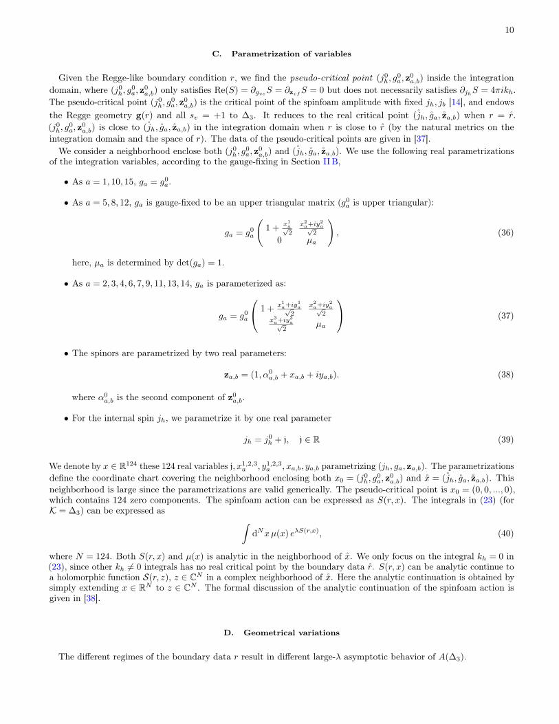
TABLE VIII. Deficit angles δh and corresponding absolute errorsδh 2× 10−16 1.8× 10−14 1.6× 10−13 1.4× 10−12 1.0× 10−10 1.8× 10−9 1.6× 10−8 1.6× 10−5 2× 10−5 0.0002ε 4.3× 10−79 2.5× 10−69 1.4× 10−64 7.1× 10−60 1.3× 10−50 2.5× 10−44 1.4× 10−39 1.4× 10−24 4.2× 10−24 4.2× 10−19

F. Flipping orientations and numerical results

So far we only consider one real critical point with all sv = +1. When we take into account different orientations ofeach 4-simplex v, there is another real critical point with all sv = −1. Other 6 discontinuous orientations violate theflatness constraint γδsh = γ

∑v svΘh(v) = 0 thus do not correspond to any real critical point. Given r, Table IX lists

δsh’s at different orientations.

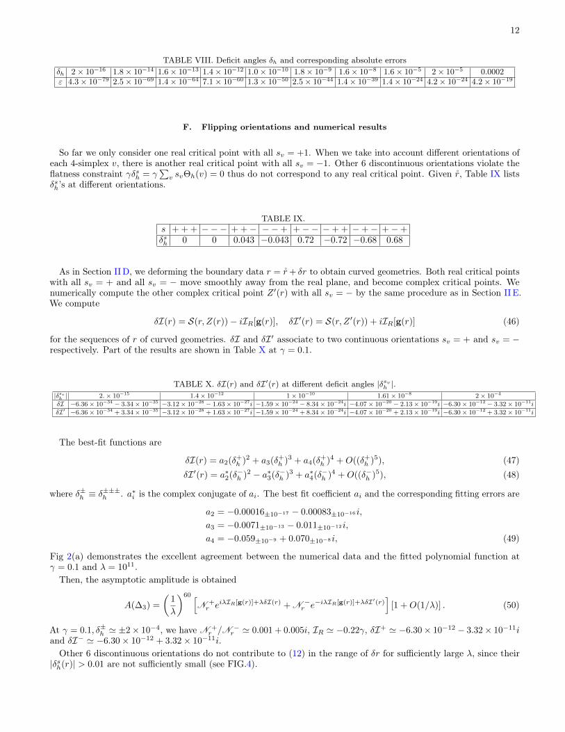
TABLE IX.s + + + −−− + +− −−+ +−− −+ + −+− +−+δsh 0 0 0.043 −0.043 0.72 −0.72 −0.68 0.68

As in Section IID, we deforming the boundary data r = r+ δr to obtain curved geometries. Both real critical pointswith all sv = + and all sv = − move smoothly away from the real plane, and become complex critical points. Wenumerically compute the other complex critical point Z ′(r) with all sv = − by the same procedure as in Section II E.We compute

δI(r) = S(r, Z(r))− iIR[g(r)], δI ′(r) = S(r, Z ′(r)) + iIR[g(r)] (46)

for the sequences of r of curved geometries. δI and δI ′ associate to two continuous orientations sv = + and sv = −respectively. Part of the results are shown in Table X at γ = 0.1.

TABLE X. δI(r) and δI′(r) at different deficit angles |δsvh |.|δsvh | 2.× 10−15 1.4× 10−12 1× 10−10 1.61× 10−8 2× 10−4

δI −6.36× 10−34 − 3.34× 10−35 −3.12× 10−28 − 1.63× 10−27i −1.59× 10−24 − 8.34× 10−24i −4.07× 10−20 − 2.13× 10−19i −6.30× 10−12 − 3.32× 10−11iδI′ −6.36× 10−34 + 3.34× 10−35 −3.12× 10−28 + 1.63× 10−27i −1.59× 10−24 + 8.34× 10−24i −4.07× 10−20 + 2.13× 10−19i −6.30× 10−12 + 3.32× 10−11i

The best-fit functions are

δI(r) = a2(δ+h )2 + a3(δ+

h )3 + a4(δ+h )4 +O((δ+

h )5), (47)δI ′(r) = a∗2(δ−h )2 − a∗3(δ−h )3 + a∗4(δ−h )4 +O((δ−h )5), (48)

where δ±h ≡ δ±±±h . a∗i is the complex conjugate of ai. The best fit coefficient ai and the corresponding fitting errors are

a2 = −0.00016±10−17 − 0.00083±10−16i,

a3 = −0.0071±10−13 − 0.011±10−12i,

a4 = −0.059±10−9 + 0.070±10−8i, (49)

Fig 2(a) demonstrates the excellent agreement between the numerical data and the fitted polynomial function atγ = 0.1 and λ = 1011.

Then, the asymptotic amplitude is obtained

A(∆3) =

(1

λ

)60 [N +r eiλIR[g(r)]+λδI(r) + N −

r e−iλIR[g(r)]+λδI′(r)]

[1 +O(1/λ)] . (50)

At γ = 0.1, δ±h ' ±2× 10−4, we have N +r /N −

r ' 0.001 + 0.005i, IR ' −0.22γ, δI+ ' −6.30× 10−12 − 3.32× 10−11iand δI− ' −6.30× 10−12 + 3.32× 10−11i.Other 6 discontinuous orientations do not contribute to (12) in the range of δr for sufficiently large λ, since their

|δsh(r)| > 0.01 are not sufficiently small (see FIG.4).

13

FIG. 4. The Log-Log plot of |δsh| for different s = svv when varying l26 = l26 + δl26.

III. 1-5 PACHNER MOVE AND A(σ1-5)

A. Flat geometry, boundary data, and real critial point

The triangulation σ1-5 of the 1-5 pachner move is made by five 4-simplices. σ1-5 is obtained by adding an point6 inside a 4-simplex and connecting 6 to other 5 points of the 4-simplex by 5 line segments (1, 6), (2, 6), · · · , (5, 6).See Fig.1(b). The dual cable diagram of σ1-5 is in Fig.3(b) 3 (see also [34]). σ1-5 consists of 10 boundary triangles b(dual to black strands in Fig. 3(b)) and 10 internal triangles h (dual to colored loops in Fig. 3(b)). Here, we set thecoordinates of P1, P2, P3, P4, P5 the same as Eq.(25). The coordinate of the point 6 is

P6 = (−0.068,−0.27,−0.50,−1.30) , (51)

P1, · · · , P6 determines a flat Regge geometry on σ1-5. We obtain five Lorentzian 4-simplices,S12346, S12356, S12456, S13456, S23456 with all tetrahedra and triangles space-like. The lengths of the internalline segments are l16 ≈ 2.01, l26 ≈ 6.66, l36 ≈ 4.72, l46 ≈ 0.54, l56 ≈ 6.19. The 4-d normals are determined by Eq.(25).For convenience, we choose (Na)µ with a = 2, 6, 13, 18, 23 to be (−1, 0, 0, 0) as reference for each 4-simplex. Hence, the4-d normals (Na)µ in each 4-simplex are given by:

• The first 4-simplex 12346:

N1 = (1.02,−0.06, 0.17, 0), N2 = (−1, 0, 0, 0), N3 = (−1.15, 0.07,−0.53, 0.19),

N4 = (1.50, 0.98,−0.54, 0), N5 = (−1.04, 0.06,−0.28,−0.06).

• The second 4-simplex 12356:

N6 = (−1, 0, 0, 0), N7 = (1.02,−0.06, 0.17, 0), N8 = (1.00,−0.03,−0.04, 0.07),

N9 = (1.03, 0.26, 0, 0), N10 = (1.00,−0.02,−0.02,−0.04).

• The third 4-simplex 12456:

N11 = (1.0,−0.091,−0.13, 0.22), N12 = (1.3,−0.11, 0.79,−0.28), N13 = (−1, 0, 0, 0),

N14 = (1.1, 0.50, 0.077,−0.13), N15 = (−1.5, 0.14, 0.19,−1.1).

• The fourth 4-simplex 13456:

N16 = (1.0, 0.10, 0, 0), N17 = (−1.2,−0.57, 0.30, 0), N18 = (−1, 0, 0, 0),

3 For convenience, the indexes of group variables in FIG. 3(b) are a = 1, 2, · · · , 25, the corresponding tetrahedra e are labeled by thenumbers in FIG.1(b). The correspondence are: g1 → e1,2,3,4, g2 → e1,2,3,6, g3 → e1,2,4,6, g4 → e1,3,4,6, g5 → e2,3,4,6, g6 → e1,2,3,5,g7 → e1,2,3,6, g8 → e1,2,5,6, g9 → e1,3,5,6, g10 → e2,3,5,6, g11 → e1,2,4,5, g12 → e1,2,4,6, g13 → e1,2,5,6, g14 → e1,4,5,6, g15 → e2,4,5,6,g16 → e1,3,4,5, g17 → e1,3,4,6, g18 → e1,3,5,6, g19 → e1,4,5,6, g20 → e3,4,5,6, g21 → e2,3,4,5, g22 → e2,3,4,6, g23 → e2,3,5,6, g24 → e2,4,5,6,g25 → e3,4,5,6.

14

N19 = (−1.0,−0.19,−0.029, 0.049), N20 = (−1.0,−0.14,−0.012,−0.020).

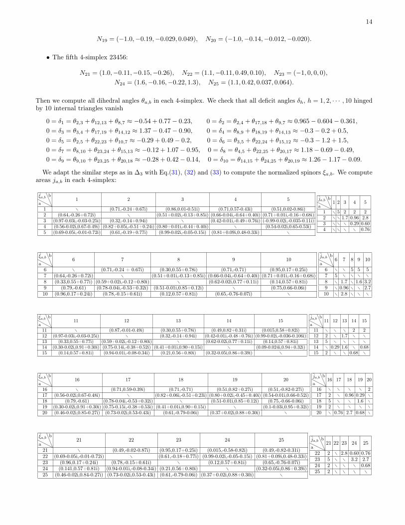
• The fifth 4-simplex 23456:

N21 = (1.0,−0.11,−0.15,−0.26), N22 = (1.1,−0.11, 0.49, 0.10), N23 = (−1, 0, 0, 0),

N24 = (1.6,−0.16,−0.22, 1.3), N25 = (1.1, 0.42, 0.037, 0.064).

Then we compute all dihedral angles θa,b in each 4-simplex. We check that all deficit angles δh, h = 1, 2, · · · , 10 hingedby 10 internal triangles vanish

0 = δ1 = θ2,3 + θ12,13 + θ8,7 ≈ −0.54 + 0.77− 0.23, 0 = δ2 = θ2,4 + θ17,18 + θ9,7 ≈ 0.965− 0.604− 0.361,

0 = δ3 = θ3,4 + θ17,19 + θ14,12 ≈ 1.37− 0.47− 0.90, 0 = δ4 = θ8,9 + θ18,19 + θ14,13 ≈ −0.3− 0.2 + 0.5,

0 = δ5 = θ2,5 + θ22,23 + θ10,7 ≈ −0.29 + 0.49− 0.2, 0 = δ6 = θ3,5 + θ22,24 + θ15,12 ≈ −0.3− 1.2 + 1.5,

0 = δ7 = θ8,10 + θ23,24 + θ15,13 ≈ −0.12 + 1.07− 0.95, 0 = δ8 = θ4,5 + θ22,25 + θ20,17 ≈ 1.18− 0.69− 0.49,

0 = δ9 = θ9,10 + θ23,25 + θ20,18 ≈ −0.28 + 0.42− 0.14, 0 = δ10 = θ14,15 + θ24,25 + θ20,19 ≈ 1.26− 1.17− 0.09.

We adapt the similar steps as in ∆3 with Eq.(31), (32) and (33) to compute the normalized spinors ξa,b. We computeareas ja,b in each 4-simplex:

a

ξa,b b1 2 3 4 5

1 (0.71,-0.24+0.67i) (0.86,0.01-0.51i) (0.71,0.57-0.43i) (0.51,0.02-0.86i)2 (0.64,-0.26+0.72i) (0.51+0.02i,-0.13+0.85i) (0.66-0.04i,-0.64+0.40i) (0.71+0.01i,-0.16+0.68i)3 (0.97-0.03i,-0.03-0.25i) (0.32,-0.14+0.94i) (0.42-0.01i,-0.49+0.76i) (-0.99-0.02i,-0.035-0.11i)4 (0.56-0.02i,0.67-0.49i) (0.82+0.05i,-0.51+0.24i) (0.80+0.01i,-0.44+0.40i) (0.54-0.02i,0.65-0.53i)5 (0.69-0.05i,-0.01-0.72i) (0.61,-0.19+0.77i) (0.99-0.02i,-0.05-0.15i) (0.81+0.09i,0.48-0.33i)

a

ja,b b1 2 3 4 5

1 5 2 2 22 1.7 0.96 2.83 0.29 0.604 0.76

a

ξa,b b6 7 8 9 10

6 (0.71,-0.24 + 0.67i) (0.30,0.55+0.78i) (0.71,-0.71) (0.95,0.17+0.25i)7 (0.64,-0.26+0.72i) (0.51+0.01i,-0.13+0.85i) (0.66-0.04i,-0.64+0.40i) (0.71+0.01i,-0.16+0.68i)8 (0.33,0.55+0.77i) (0.59+0.02i,-0.12+0.80i) (0.62-0.02i,0.77+0.11i) (0.14,0.57+0.81i)9 (0.79,-0.61) (0.78-0.04i,-0.53+0.32i) (0.51-0.01i,0.85+0.12i) (0.75,0.66-0.06i)10 (0.96,0.17+0.24i) (0.78,-0.15+0.61i) (0.12,0.57+0.81i) (0.65,-0.76-0.07i)

a

ja,b b6 7 8 9 10

6 5 5 57 58 1.7 1.6 3.29 0.96 2.710 2.8

a

ξa,b b11 12 13 14 15

11 (0.87,-0.01-0.49i) (0.30,0.55+0.78i) (0.49,0.82+0.31i) (0.015,0.58+0.82i)12 (0.97-0.03i,-0.03-0.25i) (0.32,-0.14+0.94i) (0.42-0.01i,-0.48+0.76i) (0.99-0.02i,-0.036-0.106i)13 (0.33,0.55+0.77i) (0.59+0.02i,-0.12+0.80i) (0.62-0.02i,0.77+0.11i) (0.14,0.57+0.81i)14 (0.30-0.02i,0.91+0.30i) (0.75-0.14i,-0.38+0.52i) (0.41+0.01i,0.90+0.15i) (0.09-0.024i,0.94+0.32i)15 (0.14,0.57+0.81i) (0.94-0.01i,-0.08-0.34i) (0.21,0.56+0.80i) (0.32-0.05i,0.86+0.39i)

a

ja,b b11 12 13 14 15

11 2 212 2 1.713 514 0.29 1.6 0.6815 2 0.68

a

ξa,b b16 17 18 19 20

16 (0.71,0.59-0.39i) (0.71,-0.71) (0.51,0.82+0.27i) (0.51,-0.82-0.27i)17 (0.56-0.02i,0.67-0.48i) (0.82+0.06i,-0.51+0.23i) (0.80+0.02i,-0.45+0.40i) (0.54-0.01i,0.66-0.52i)18 (0.79,-0.61) (0.78-0.04i,-0.53+0.32i) (0.51-0.01i,0.85+0.12i) (0.75,-0.66-0.06i)19 (0.30-0.02i,0.91+0.30i) (0.75-0.15i,-0.38+0.53i) (0.41+0.01i,0.90+0.15i) (0.1-0.03i,0.95+0.32i)20 (0.46-0.02i,0.85-0.27i) (0.73-0.02i,0.53-0.43i) (0.61,-0.79-0.06i) (0.37+0.02i,0.88+0.30i)

a

ja,b b16 17 18 19 20

16 217 2 0.96 0.2918 5 1.619 220 0.76 2.7 0.68

a

ξa,b b21 22 23 24 25

21 (0.49,-0.02-0.87i) (0.95,0.17+0.25i) (0.015,-0.58-0.82i) (0.49,-0.82-0.31i)22 (0.69-0.05i,-0.01-0.72i) (0.61,-0.18+0.77i) (0.99-0.02i,-0.05-0.15i) (0.81+0.09i,0.48-0.33i)23 (0.96,0.17+0.24i) (0.78,-0.15+0.61i) (0.12,0.57+0.81i) (0.65,-0.76-0.07i)24 (0.141,0.57+0.81i) (0.94-0.01i,-0.08-0.34i) (0.21,0.56+0.80i) (0.32-0.05i,0.86+0.39i)25 (0.46-0.02i,0.84-0.27i) (0.73-0.02i,0.53-0.43i) (0.61,-0.79-0.06i) (0.37+0.02i,0.88+0.30i)

a

ja,b b21 22 23 24 25

22 2 2.8 0.60 0.7623 5 3.2 2.724 2 0.6825 2

15

The boundary data r = jb, ξeb are given in the above tables. The real critical point (jh, ga, za,b) correspondingto the above flat Regge geometry are obtained by solving critical point equations Eqs. (5) and (6). To remove thegauge freedom, We choose ga, a = 1, 6, 11, 16, 21, to be identity and ga, a = 2, 3, 8, 9, 14, 15, 17, 20, 22, 23, to be uppertriangular matrix. In each 4-simplex, we choose a = 1, 6, 11, 16, 21 as the references and use Eq.(34) to obtain criticalpoints ga. The resulting ga and za,b are given below. jh are given by ja,b’s of the internal triangles in the above tables.The critical point endows the continuous orientation sv = −1 to all 4-simplices.

a 1 2 3

ga

(1.02 −0.06− 0.17i

−0.06 + 0.17i 1.02

) (0.99 −0.06− 0.17i

0 1.01

) (0.83 −0.12− 0.61i

0 1.20

)a 4 5

ga

(0.99 0.55 + 0.29i0.25 1.14 + 0.074i

) (0.94 −0.12− 0.45i

0 1.02

)a|za,b〉 b

2 3 4 5

1 (1,-0.33 + 0.94 i) (1,0.08 - 0.69 i) (0.68 - 0.73i) (1,0.18 - 1.43 i)2 (1,-0.14 + 1.50 i) (1,-0.93 + 0.37i) (1,-0.16 + 0.77i)3 (1,-0.93 + 0.48i) (1,0.078 - 0.58 i)4 (1,0.64 - 0.88i)

a 6 7 8

ga

(1 00 1

) (0.99 −0.06− 0.17i

0 1.01

) (1.03 −0.03 + 0.045i

0 0.96

)a 9 10

ga

(0.98 0.25

0 1.02

) (0.98 −0.02 + 0.02i

0 1.02

)a|za,b〉 b

6 7 8 9 10

6 (1,1.82 + 2.57i) (1,-1) (0.18 + 0.26i)7 (1,-0.33 + 0.94i)8 (1,-0.14+ 1.50i) (1,1.36 + 0.27i) (1,4.60 + 6.50i)9 (1,-0.93 + 0.37i) (1,-1.11 - 0.072i)10 (1,-0.16 + 0.77i)

a 11 12 13

ga

(1.08 −0.03 + 0.04i

−0.03− 0.04i 0.93

) (0.77 −0.08− 0.62i

0.02 + 0.04i 1.32− 0.02i

) (0.96 0

0.03 + 0.04i 1.04

)a 14 15

ga

(0.85 0.45− 0.11i

0 1.18

) (1.52 −0.14 + 0.2i

0 0.66

)a|za,b〉 b

11 12 13 14 15

11 (1,1.77 + 0.80i) (1,9.6 + 13.58i)12 (1,0.03 - 0.62i) (1,-0.23 + 1.31i)13 (1,1.82 + 2.57i)14 (1,-0.84 + 0.33i) (1,1.21 + 0.14i) (1,5.92 + 4.04i)15 (1,0.027 - 0.53i) (1,6.48 + 9.17i)

a 16 17 18

ga

(1.00 −0.07−0.07 1.00

) (0.96 0.27 + 0.28i

0 1.04

) (1.02 0−0.26 0.98

)a 19 20

ga

(0.96 + 0.01i 0.19− 0.06i−0.26− 0.38i 0.99

) (1.01 −0.12− 0.01i

0 0.99

)a|za,b〉 b

16 17 18 19 20

16 (1,-1.7 - 0.68i)17 (1,0.87 - 0.48i) (1,-0.82 + 0.58i) (1,-0.76 + 0.75i)18 (1,-1) (1,1.21 + 0.14i)19 (1,1.51 + 0.42i)20 (1,0.88 - 0.59i) (1,-1.20 - 0.13i) (1,2.54 + 0.65i)

a 21 22 23

ga

(0.87 −0.06 + 0.086i

−0.06− 0.085i 1.16

) (0.97 −0.13− 0.45i

0 1.03

) (0.98 −0.016 + 0.023i

0 1.02

)a 24 25

ga

(1.64 −0.17 + 0.24i

−0.05− 0.07i 0.62

) (1.04 −0.14− 0.01i0.26 0.99− 0.003i

)a|za,b〉 b

21 23 24 25

22 (1,0.18 - 1.43i) (1,-0.15 + 0.78i) (1,0.078 - 0.58i) (1,0.64 - 0.88i)23 (1,0.18 + 0.26i) (1,4.6 + 6.5i) (1,-1.11 - 0.072i)24 (1,5.72 + 8.08i) (1,4.58 + 3.90i)25 (1,-1.41 - 0.31i)

The flat geometry on σ1-5 is not unique. The position of P6 can move continuously in R4 to lead to the continuousfamily of flat geometries on σ1-5. The continuous family of flat geometries result in the continuous family of real criticalpoints. It implies that all these real critical points lead to degenerate Hessian matrices, in contrast to A(∆3) where thereal critical point is nondegenerate. Therefore we develop the following additional procedure to generalize the analysisfrom ∆3 to σ1-5.We label boundary spins jmnk by a triple of points m 6= n 6= k = 1, 2, · · · , 5, and label the internal spins jmn6 by

m,n = 1, 2, · · · , 5 and point 6. The dual faces and spins are labelled in the dual cable diagram Fig.3(b). We pick up5 internal spins j126, j136, j146, j156, j236 and their corresponding integrals in A(σ1-5). The integrand is denoted byZσ1-5 . Namely

A(σ1-5) =

∫R5

dj126dj136dj146dj156dj236Zσ1-5 (j126, j136, j146, j156, j236) , (52)

Zσ1-5 =∑kh

∫R5

5∏h=1

djh

10∏h=1

2λ τ[−ε,λjmax+ε](λjh)

∫[dgdz]eλS

(k)

, (53)

where other five internal spins j246, j256, j346, j356, j456 are denoted by jh (h = 1, 2, · · · , 5). At the real criticalpoint constructed above, the 5 areas j126, j136, j146, j156, j236 are determined by the internal segment-lengths lm6

16

(m = 1, 2, · · · , 5) via the Heron’s formula. We focus on a neighborhood of (j126, j136, j146, j156, j236) ∈ R5 around(j126, j136, j146, j156, j236) such that the five j’s in the neighborhood uniquely correspond to the five segment-lengthslm6, m = 2, · · · , 5.

We generalize the analysis of A(∆3) to Zσ1-5 . Zσ1-5 in Eq.(53) contain integrals with the external parameters

r = j126, j136, j146, j156, j236, jb, ξeb (54)

which including not only boundary data but also 5 internal j’s. We focus on the integral in Zσ1-5 at kh = 0. Givenr = r = j126, j136, j146, j156, j236, jb, ξeb, the integral has the real critical point jh, ga, za,b corresponding to theflat geometry g(r). The data of r and the real critical point are given in the above tables. The Hessian matrix at x isnondegenerate in Zσ1-5 .The similar parametrizations as Eq.(36), (37), (38), and (39) for ga, za,b, jh define the local coordinates x ∈ R195

covering a neighborhood K of x = (0, 0, · · · , 0). We again express the spinfoam action as S(r, x). The integral in Zσ1-5

is of the same type as (40) with N = 195.

B. Geometrical variations

All the above data relate to the real critical point and the flat geometry with 10 deficit angles all zero. To givethe curved geometries, we fix the boundary data jb, ξeb and deform the 5 internal segment-lengths lm6 = lm6 + δlm6,m = 1, · · · , 5. We randomly sample δlm6 in the range 10−15 to 10−5. Each time, for the each new internal segment-lengths lm6, we can solve for the coordinate P6. Then, we repeat the procedure above to reconstruct the geometry andcompute all the geometric quantities of triangulation: e.g. the areas, the 4-d normals of each tetrahedron, and thedeficit angles. Some data of the deformation δlm6 = (δl16, δl26, δl36, δl46, δl56) and the corresponding deficit angles δhare shown in Tables XI and XII,

TABLE XI. Deficit angles as δlm6 = (3.0× 10−6, 3.7× 10−6,−3.1× 10−6,−2.8× 10−6,−3.6× 10−6)

δ1 δ2 δ3 δ4 δ5 δ6 δ7 δ8 δ9 δ10 δ6.1× 10−5 2.6× 10−4 1.1× 10−4 1.4× 10−4 4.6× 10−5 1.4× 10−5 1.8× 10−5 1.3× 10−4 1.1× 10−4 4.1× 10−5 1.2× 10−4

TABLE XII. Deficit angles as δlm6 = (−3.× 10−8, 5.0× 10−8, 3.4× 10−8, 3.1× 10−8, 4.0× 10−8)

δ1 δ2 δ3 δ4 δ5 δ6 δ7 δ8 δ9 δ10 δ1.5× 10−6 6.4× 10−6 2.8× 10−6 3.5× 10−6 1.1× 10−6 3.6× 10−7 4.5× 10−7 3.3× 10−6 2.8× 10−6 1.0× 10−6 2.9× 10−6

Here δ is the average deficit angle δ =√

110

∑10h=1 δ

2h.

Fixing jb, ξeb, varying lm6 = lm6+δlm6 results in varying the 5 areas in r e.g. j126 = j126+δj126, j136 = j136+δj136, · · · .Thus we obtain the deformation of external data r = r + δr of Zσ1-5 . We denote by rl the external data obtained bysampling δlm6, and denote the Regge geometries by g(rl). There are 4 degrees of freedom of δlm6 still resulting in flatgeometries, whereas there is 1 degree of freedom of δlm6 resulting in curved geometries.

C. Complex critical points and numerical results

We apply the Newton-like recursive method similar to Section II E to numerically compute complex critical pointsZ(rl) for all rl. The absolute errors in the case γ = 1, n = 3 for some average deficit angles are shown in Table III C.

δ 1.2× 10−4 1.2× 10−5 2.1× 10−6 6.5× 10−7 1.3× 10−8 1.2× 10−10 1.5× 10−11 1.4× 10−12

ε 4.0× 10−15 2.1× 10−19 2.0× 10−22 2.0× 10−27 2.3× 10−31 2.3× 10−39 5.0× 10−43 5.0× 10−47

Z(rl) is still in the real plane if rl corresponds to the flat geometry, whereas Z(rl) is away from the real plane if rlcorresponds to the curved geometry.Once we have complex critical points Z(rl) for the curved geometries g(rl), we numerically compute the analytic

continued action S(rl, Z(rl)) at complex critical points and the difference δI(rl) = S(rl, Z(rl))− S(rl, x0) where x0 isthe pseudo-critical point of S(rl, x) (recall Section II E). We have S(rl, x0) = −iIR[g(r)] + iϕ, where ϕ only relates tothe boundary data and is independent of lm6 as confirmed by numerical tests (see also [14] for the analytic argument).Some numerical results of δI are shown in Table III C

17

δ 1.2× 10−4 2.1× 10−6 3.8× 10−8 6.5× 10−10 6.5× 10−12

δI −1.2× 10−12 + 4.5× 10−10i −3.8× 10−16 + 1.4× 10−13i −1.3× 10−19 + 4.7× 10−17i −3.8× 10−23 + 1.4× 10−20i −3.8× 10−27 + 1.4× 10−24i

The best-fit function is δI = −a2(γ)δ2 +O(δ3), the best fit coefficient and the corresponding fitting errors at γ = 1is:

a2 = 8.88× 10−5±10−12 − i0.033±10−10 . (55)

We use FIG.2(b) to demonstrate the excellent agreement between the numerical data and the best-fit function.As a result, we obtain the following large-λ contribution to Zσ1-5 and A(σ1-5) from the neighborhood around (r, x)

Zσ1-5 ∼(

1

λ

) 1552

eiλϕN ′l e−iλIR[g(rl)]−λa2(γ)δ(rl)

2+O(δ3) [1 +O(1/λ)] , (56)

A(σ1-5) ∼(

1

λ

) 1552

eiλϕ∫ 5∏

m=1

dlm6Nl e−iλIR[g(rl)]−λa2(γ)δ(rl)

2+O(δ3) [1 +O(1/λ)] , (57)

where we have made the local changes of variables from j126, j136, j146, j156, j236 to lm6, and the Jacobian Jl =|det(∂j/∂l)| is absorbed in Nl = JlN ′

l . The spinfoam amplitude A(σ1-5) reduces to the integral over geometries g(rl)in the semiclassical regime.

The Jacobian Jl reads:

l16l26l36l46l56(l214 + l216 − l246

)(l215 + l216 − l256

) [(l216 − l236

) (l226 − l236

)− l213l223

]l212 +

(l216 − l226

) [(l236 − l226

)l213 + l223

(l216 − l236

)]16√−l412 + 2 (l216 + l226) l212 − (l216 − l226) 2

√−l413 + 2 (l216 + l236) l213 − (l216 − l236) 2

√−l423 + 2 (l226 + l236) l223 − (l226 − l236) 2

1√−l414 + 2 (l216 + l246) l214 − (l216 − l246) 2

√−l415 + 2 (l216 + l256) l215 − (l216 − l256) 2

.

[1] T. Thiemann, Modern Canonical Quantum General Relativity. Cambridge Monographs on Mathematical Physics.Cambridge University Press, 2007.

[2] C. Rovelli and F. Vidotto, Covariant Loop Quantum Gravity: An Elementary Introduction to Quantum Gravity andSpinfoam Theory. Cambridge Monographs on Mathematical Physics. Cambridge University Press, 11, 2014.

[3] A. Perez, The Spin Foam Approach to Quantum Gravity, Living Rev.Rel. 16 (2013) 3, [arXiv:1205.2019].[4] C. Rovelli, Loop quantum gravity: the first twenty five years, Class. Quant. Grav. 28 (2011) 153002, [arXiv:1012.4707].[5] A. Ashtekar and J. Pullin, eds., Loop Quantum Gravity: The First 30 Years, vol. 4 of 100 Years of General Relativity.

World Scientific, 2017.[6] A. Ashtekar and E. Bianchi, A short review of loop quantum gravity, Rept. Prog. Phys. 84 (2021), no. 4 042001,

[arXiv:2104.04394].[7] J. Engle, R. Pereira, and C. Rovelli, The Loop-quantum-gravity vertex-amplitude, Phys. Rev. Lett. 99 (2007) 161301,

[arXiv:0705.2388].[8] J. Engle, E. Livine, R. Pereira, and C. Rovelli, LQG vertex with finite Immirzi parameter, Nucl. Phys. B 799 (2008)

136–149, [arXiv:0711.0146].[9] C. Rovelli, Graviton propagator from background-independent quantum gravity, Phys. Rev. Lett. 97 (2006) 151301,

[gr-qc/0508124].[10] E. R. Livine and S. Speziale, A New spinfoam vertex for quantum gravity, Phys. Rev. D 76 (2007) 084028,

[arXiv:0705.0674].[11] L. Freidel and K. Krasnov, A New Spin Foam Model for 4d Gravity, Class. Quant. Grav. 25 (2008) 125018,

[arXiv:0708.1595].[12] F. Conrady and L. Freidel, On the semiclassical limit of 4d spin foam models, Phys. Rev. D78 (2008) 104023,

[arXiv:0809.2280].[13] J. W. Barrett, R. J. Dowdall, W. J. Fairbairn, F. Hellmann, and R. Pereira, Lorentzian spin foam amplitudes: Graphical

calculus and asymptotics, Class. Quant. Grav. 27 (2010) 165009, [arXiv:0907.2440].[14] M. Han and M. Zhang, Asymptotics of Spinfoam Amplitude on Simplicial Manifold: Lorentzian Theory, Class. Quant.

Grav. 30 (2013) 165012, [arXiv:1109.0499].[15] M. Han and T. Krajewski, Path Integral Representation of Lorentzian Spinfoam Model, Asymptotics, and Simplicial

Geometries, Class. Quant. Grav. 31 (2014) 015009, [arXiv:1304.5626].[16] W. Kaminski, M. Kisielowski, and H. Sahlmann, Asymptotic analysis of the EPRL model with timelike tetrahedra, Class.

Quant. Grav. 35 (2018), no. 13 135012, [arXiv:1705.02862].[17] H. Liu and M. Han, Asymptotic analysis of spin foam amplitude with timelike triangles, Phys. Rev. D 99 (2019), no. 8

084040, [arXiv:1810.09042].

18

[18] J. D. Simão and S. Steinhaus, Asymptotic analysis of spin-foams with time-like faces in a new parameterisation,arXiv:2106.15635.

[19] P. Dona and S. Speziale, Asymptotics of lowest unitary SL(2,C) invariants on graphs, Phys. Rev. D 102 (2020), no. 8086016, [arXiv:2007.09089].

[20] J. S. Engle, W. Kaminski, and J. R. Oliveira, Addendum to ‘EPRL/FK asymptotics and the flatness problem’,arXiv:2012.14822. [Addendum: Class.Quant.Grav. 38, 119401 (2021)].

[21] F. Hellmann and W. Kaminski, Geometric asymptotics for spin foam lattice gauge gravity on arbitrary triangulations,arXiv:1210.5276.

[22] V. Bonzom, Spin foam models for quantum gravity from lattice path integrals, Phys. Rev. D 80 (2009) 064028,[arXiv:0905.1501].

[23] M. Han, On Spinfoam Models in Large Spin Regime, Class. Quant. Grav. 31 (2014) 015004, [arXiv:1304.5627].[24] F. Gozzini, A high-performance code for EPRL spin foam amplitudes, arXiv:2107.13952.[25] J. Engle, The Plebanski sectors of the EPRL vertex, Class. Quant. Grav. 28 (2011) 225003, [arXiv:1301.2214]. [Erratum:

Class.Quant.Grav. 30, 049501 (2013)].[26] C. Rovelli and L. Smolin, Discreteness of area and volume in quantum gravity, Nuclear Physics B 442 (May, 1995) 593–619.[27] A. Ashtekar and J. Lewandowski, Quantum theory of geometry. 1: Area operators, Class.Quant.Grav. 14 (1997) A55–A82,

[gr-qc/9602046].[28] A. Melin and J. Sjöstrand, Fourier integral operators with complex-valued phase functions, in Fourier Integral Operators and

Partial Differential Equations (J. Chazarain, ed.), (Berlin, Heidelberg), pp. 120–223, Springer Berlin Heidelberg, 1975.[29] L. Hormander, The Analysis of Linear Partial Differential Operators I. Springer-Verlag Berlin, 1983.[30] P. Dona, F. Gozzini, and G. Sarno, Numerical analysis of spin foam dynamics and the flatness problem, arXiv:2004.12911.[31] S. K. Asante, B. Dittrich, and H. M. Haggard, Effective Spin Foam Models for Four-Dimensional Quantum Gravity, Phys.

Rev. Lett. 125 (2020), no. 23 231301, [arXiv:2004.07013].[32] B. Bahr and S. Steinhaus, Numerical evidence for a phase transition in 4d spin foam quantum gravity, Phys. Rev. Lett. 117

(2016), no. 14 141302, [arXiv:1605.07649].[33] C. Delcamp and B. Dittrich, Towards a phase diagram for spin foams, Class. Quant. Grav. 34 (2017), no. 22 225006,

[arXiv:1612.04506].[34] A. Banburski, L.-Q. Chen, L. Freidel, and J. Hnybida, Pachner moves in a 4d Riemannian holomorphic Spin Foam model,

Phys. Rev. D 92 (2015), no. 12 124014, [arXiv:1412.8247].[35] M. Han, Z. Huang, H. Liu, and D. Qu, Numerical computations of next-to-leading order corrections in spinfoam large-j

asymptotics, Phys. Rev. D 102 (2020), no. 12 124010, [arXiv:2007.01998].[36] P. Dona, M. Fanizza, G. Sarno, and S. Speziale, Numerical study of the Lorentzian Engle-Pereira-Rovelli-Livine spin foam

amplitude, Phys. Rev. D100 (2019), no. 10 106003, [arXiv:1903.12624].[37] D. Qu.

https://github.com/dqu2017/Complex-critical-points-and-curved-geometries-in-spinfoam-quantum-gravity,2021.

[38] M. Han and H. Liu, Analytic Continuation of Spin foam Models, 4, 2021. arXiv:2104.06902.