12. coordinate geometry...12. coordinate geometry the cartesian plane we recall from our study of...

www.fasp

assm

aths.c

om

95

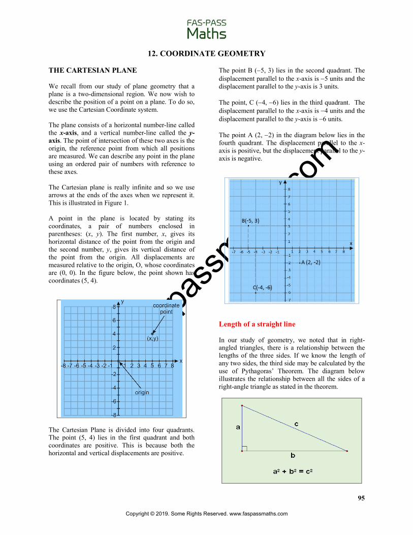
12. COORDINATE GEOMETRY THE CARTESIAN PLANE We recall from our study of plane geometry that a plane is a two-dimensional region. We now wish to describe the position of a point on a plane. To do so, we use the Cartesian Coordinate system. The plane consists of a horizontal number-line called the x-axis, and a vertical number-line called the y-axis. The point of intersection of these two axes is the origin, the reference point from which all positions are measured. We can describe any point in the plane using an ordered pair of numbers with reference to these axes. The Cartesian plane is really infinite and so we use arrows at the ends of the axes when we represent it. This is illustrated in Figure 1. A point in the plane is located by stating its coordinates, a pair of numbers enclosed in parentheses: (x, y). The first number, x, gives its horizontal distance of the point from the origin and the second number, y, gives its vertical distance of the point from the origin. All displacements are measured relative to the origin, O, whose coordinates are (0, 0). In the figure below, the point shown has coordinates (5, 4).

The Cartesian Plane is divided into four quadrants. The point (5, 4) lies in the first quadrant and both coordinates are positive. This is because both the horizontal and vertical displacements are positive.

The point B (-5, 3) lies in the second quadrant. The displacement parallel to the x-axis is -5 units and the displacement parallel to the y-axis is 3 units. The point, C (-4, -6) lies in the third quadrant. The displacement parallel to the x-axis is -4 units and the displacement parallel to the y-axis is -6 units. The point A (2, -2) in the diagram below lies in the fourth quadrant. The displacement parallel to the x-axis is positive, but the displacement parallel to the y-axis is negative.

Length of a straight line In our study of geometry, we noted that in right-angled triangles, there is a relationship between the lengths of the three sides. If we know the length of any two sides, the third side may be calculated by the use of Pythagoras’ Theorem. The diagram below illustrates the relationship between all the sides of a right-angle triangle as stated in the theorem.

Copyright © 2019. Some Rights Reserved. www.faspassmaths.com

www.fasp

assm

aths.c

om

96

We will use this relationship to calculate the length of a line on the Cartesian plane from coordinates. In the diagram below, let A and B represent two points, A and B . The vertical and the horizontal distances can be calculated as follows: Vertical Side = Horizontal Side =

By Pythagoras’ Theorem, the length of the straight line is AB = If A and B represent two points, such that A and B , then the distance AB is

Example 1 Given and B = (5,7) calculate the length of AB. Solution

The length of a line is

Hence, the length of AB =

= =

= units.

Example 2 Calculate the length of PQ, where P = (1, -1) and

. Solution

Length of PQ = =

= = 6.32 units (correct to 2 dec places) As shown in the example above, the length of a line may not compute to an exact integer value and sometimes we may have to use a calculator to approximate this length to any required degree of accuracy or simply leave the exact answer in a surd form. Midpoint of a straight line If a point, M is midway between two other points A and B, its distance is the arithmetic average of the coordinates.

Since the 𝑥-coordinates of A abd B are 6 and 14 respectively, the 𝑥 coordinate of M is .

We can use this principle to determine the mid-point of any line given the coordinates of any two points on the line. Let A and B represent two points, A and B . Let the mid-point be M (𝑥,# 𝑦&). The 𝑥-coordinate of M is the average of 𝑥(and𝑥,. The 𝑦-coordinate of M is the average of 𝑦(and𝑦,.

( )1 1,x y ( )2 2,x y

2 1y y-

2 1x x-

( ) ( )2 22 1 2 1x x y y- + -

( )1 1,x y ( )2 2,x y

( ) ( )2 22 1 2 1x x y y- + -

( )2,3A=

( ) ( )2 22 1 2 1x x y y- + -

( ) ( )2 25 2 7 3- + -

( ) ( )2 23 4+

9 16+

25 5=

( )3,5Q =

( ) ( )( )223 1 5 1- + - - ( ) ( )2 22 6+

( )40 exact

6 14 102+

=

( )1 1,x y ( )2 2,x y


www.fasp

assm

aths.c

om

97

In general, the midpoint of the straight line joining and has coordinates:

.

Example 3 If and , calculate the coordinates of the mid-point of AB. Solution Applying the formula for the mid-point

.

Hence, the midpoint of AB is

Example 4

If and , calculate the

coordinates of the mid-point of PQ. Solution Midpoint if PQ

Example 5 Given that A (2,3) and M(4,5), where M is the midpoint of AB. Find the coordinates of B. Solution Let A(x1,y1) and B(x2, y2)

We recall the midpoint formula:

Therefore, B is the point with coordinates, (7, 8).

Gradient of a straight line When we speak of the gradient or the slope of a straight line, we refer to the measure of the steepness of the line. Lines can have varying degrees of steepness depending on their orientation. Consider the five lines, shown below, L1, L2 , L3 , L4 and L5. We may observe that all five lines have different degrees of steepness. Examine the lines L2, L3 and L4. If we were to order these three lines in ascending order of steepness, then we can deduce, from observation, that L2 is the least steep of all three, then L3, and after that, L4 is the steepest of all three.

L1 and L5 are special lines. L1 is a horizontal line and is regarded as having no steepness. L5 is a vertical line and has the maximum possible steepness.

In mathematics, we need to be very precise when comparing the steepness of lines. We can only do so if we measure the steepness and assign numbers to this measure. We refer to this measure of steepness, as the slope or the gradient of the straight line. We can think of gradient as a rate of change of the vertical displacement (or rise) with respect to its horizontal displacement (or run, sometimes referred to as step). When both the horizontal and vertical distances are expressed in the same units, we can express the gradient as a ratio of the rise to the run. We can think of gradient, which is often denoted by the letter m, in mathematics, as any one of the following ratios.

( )1 1,x y ( )2 2,x y

1 2 1 2,2 2

x x y y+ +æ öç ÷è ø

( )3,4A= ( )7,6B =

1 2 1 2,2 2


( )3 7 4 6, 5,52 2+ +æ ö =ç ÷

è ø

( )1, 3P = -1 ,42

Q æ ö= ç ÷è ø

11 3 42 ,2 2

æ ö+ç ÷- += ç ÷ç ÷è ø

3 1,4 2æ ö= ç ÷è ø

1 2 1 2,2 2


2

2

2

2

142

1 88 17

x

xxx

+=

+ == -=

2

2

2

2

252

2 1010 28

y

yyy

+=

+ == -=

Vertical Displacement ( )Horizontal Displacement

Gradient m =

Change in ( )Change in

yGradient mx

=


www.fasp

assm

aths.c

om

98

Calculating gradient using measurement If the line is not drawn on a grid, then we would have to take measurements (likely by a ruler) to determine the gradient.

By measurement, Vertical displacement = 3cm Horizontal displacement =5cm

Gradient from coordinates We can use the coordinates of any two points on a line to compute the gradient. This method does not require the use of a graph and it is widely used in coordinate geometry. Given A and B are any two points on the line. The vertical displacement represents a change in y values and the horizontal displacement represents a change in x values. Hence the gradient of AB is calculated as follows:

.

In general, the gradient of the straight line joining A

and B is ./0.12/021

Example Calculate the gradient of a line joining the two points (1, 4) and (6, 7).

Solution We let and represent the coordinates (1, 4) and (6, 7) respectively. We now substitute the coordinates in the formula to obtain:

Positive and negative gradient When we measure gradient, our resulting ratio can be positive or negative. The numerical value is the magnitude of the gradient and the sign (positive or negative) is the direction of the gradient. When both vertical and horizontal displacements have the same direction the gradient of the line is positive. Positive gradient Acute angle Horizontal displacement is positive Vertical displacement is positive When one of the displacements is negative, the gradient of the line is negative. Negative gradient Obtuse angle Horizontal displacement is positive Vertical displacement is negative Positive and negative gradients can also be identified by considering the angle formed with the positive x-axis. When this angle is acute the gradient is positive and when it is obtuse the gradient is negative. Notice that when the slope is positive, the angle is acute and when the slope is negative the angle is obtuse. Note also that the direction of turn is anticlockwise.

Vertical Displacement 3Gradient=Horizontal Displacement 5

=

( )1 1,x y ( )2 2,x y

2 1

2 1

Change inGradientChange in

y yyx x x

-= =

-

( )1 1,x y ( )2 2,x y

( )1 1,x y ( )2 2,x y

2 1

2 1

7 4 3Gradient6 1 5

y yx x- -

= = =- -


www.fasp

assm

aths.c

om

99

Gradient of horizontal and vertical lines The following should be noted: • A horizontal line has no steepness and its

gradient is defined as zero. This is because it has no ‘rise’ regardless of the ‘run’ and (0 ÷ any number) = 0

• A vertical line has maximum steepness and its gradient is infinite. This is because it has ‘rise’ but no ‘run’ and (any number) ÷ 0 ⟶ ∞

Horizontal lines have run, but absolutely no rise.

And so the gradient = = 0

Vertical lines have rise, but absolutely no run.

And so the gradient = = ∞

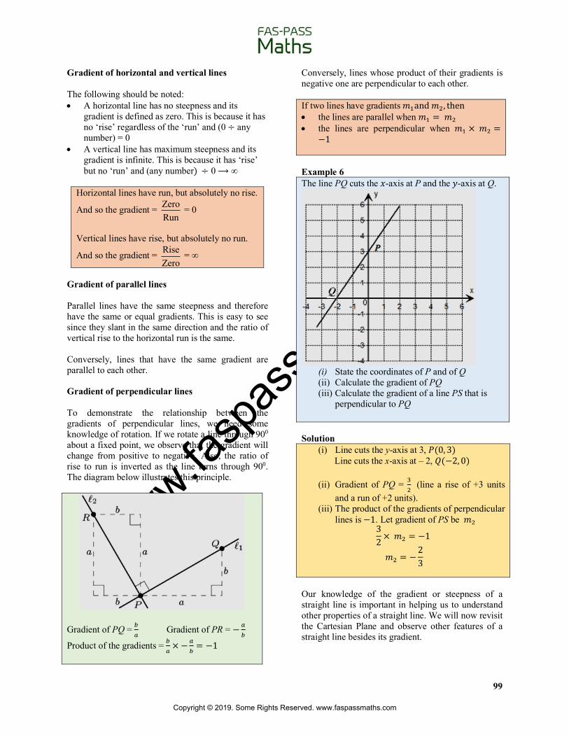
Gradient of parallel lines Parallel lines have the same steepness and therefore have the same or equal gradients. This is easy to see since they slant in the same direction and the ratio of vertical rise to the horizontal run is the same. Conversely, lines that have the same gradient are parallel to each other. Gradient of perpendicular lines To demonstrate the relationship between the gradients of perpendicular lines, we need some knowledge of rotation. If we rotate a line through 900 about a fixed point, we observe that the gradient will change from positive to negative. Also, the ratio of rise to run is inverted as the line turns through 900. The diagram below illustrates this principle.

Gradient of PQ = 5

6 Gradient of PR = −6

5

Product of the gradients = 56× −6

5 = −1

Conversely, lines whose product of their gradients is negative one are perpendicular to each other. If two lines have gradients 𝑚(and𝑚,, then • the lines are parallel when 𝑚( =𝑚, • the lines are perpendicular when 𝑚( ×𝑚, =

−1 Example 6 The line PQ cuts the 𝑥-axis at P and the 𝑦-axis at Q.

(i) State the coordinates of P and of Q (ii) Calculate the gradient of PQ (iii) Calculate the gradient of a line PS that is

perpendicular to PQ

Solution

(i) Line cuts the y-axis at 3, 𝑃(0, 3) Line cuts the x-axis at – 2, 𝑄(−2, 0) (ii) Gradient of PQ = E

, (line a rise of +3 units

and a run of +2 units). (iii) The product of the gradients of perpendicular

lines is −1. Let gradient of PS be 𝑚, 32 ×𝑚, = −1

𝑚, = −23

Our knowledge of the gradient or steepness of a straight line is important in helping us to understand other properties of a straight line. We will now revisit the Cartesian Plane and observe other features of a straight line besides its gradient.

ZeroRun

RiseZero


www.fasp

assm

aths.c

om

100

THE EQUATION OF A STRAIGHT LINE The equation of a straight line is an expression of the relationship between the x and y values in a linear equation. Let us examine a family of straight lines drawn through the origin but having different gradients.

The relationship between the x and y coordinates for each line is stated below. Equation of line Points on the line

𝑦 =12𝑥 (2, 1) (4, 2) (6, 3)

the 𝑦 −coordinate is one half of the 𝑥 −coordinate.

𝑦 = 𝑥 (1, 1) (2, 2) (3, 3) the 𝑦 −coordinate is equal to the 𝑥 −coordinate.

𝑦 = 2𝑥 (1, 2) (2, 4) (2.5, 5) the 𝑦 −coordinate is always twice the 𝑥 −coordinate.

𝑦 = 4𝑥 (0.25, 1) (0.5, 2) (1, 4) the 𝑦 −coordinate is always four times the 𝑥 −coordinate.

We now determine the gradient of each line by drawing a right-angled triangle and recording the rise over the run. This is shown below.

All the displacements are positive and so the ratio of vertical rise to horizontal run is positive. The magnitude of the gradient is recorded below. Equation of line Gradient of the line

𝑦 =12𝑥

12

𝑦 = 𝑥 1 𝑦 = 2𝑥 2 𝑦 = 4𝑥 4

By observation, the gradient of each line is the same as the coefficient of 𝑥in the equation. We are now in a position to state a rule that relates to the equation of straight lines passing through the origin. Lines passing through the origin have equations of the form 𝑦 = 𝑚𝑥, where 𝑚 is the gradient of the line. We will now examine another family of lines. These lines do not pass through the origin but they are parallel. It is easy to see that the gradient of each line is the same and equal to one.

The above lines differ in that each one passes through a different point on the y-axis. This value is called the y-intercept for each line. These values are recorded below. We may think of the line 𝑦 = 𝑥 as the base and the line 𝑦 = 𝑥 + 2 as an upward shift of shift of 2 units. Similar an upward shift of 3 units will produce the line 𝑦 = 𝑥 + 2 while a downward shift of 1 unit will produce the line 𝑦 = 𝑥 − 1. Equation of line

y-intercept

𝑦 = 𝑥 0 Line passes through the origin 𝑦 = 𝑥 + 1 1 Upward shift of 1 units. 𝑦 = 𝑥 + 3 3 Upward shift of 3 units 𝑦 = 𝑥 − 1 −1 Downward shift of 1 unit.


www.fasp

assm

aths.c

om

101

From the above table, we can conclude that the constant term in an equation of the form 𝑦 = 𝑚𝑥 + 𝑐 is the y-intercept when the line is drawn. We will now examine a new set of lines that are neither parallel nor equal in gradient.

The gradient and y-intercept for each of the four lines are shown below. Equation Gradient y-intercept

𝑦 = 𝑥 1 0 𝑦 = 2𝑥 + 1 2 1 𝑦 = 4𝑥 + 3 4 3 𝑦 = 0.5𝑥 − 1 0.5 −1

From the table, we observe the following: If the equation of a straight line is written in the form 𝑦 = 𝑚𝑥 + 𝑐, then the gradient of line is the coefficient of 𝑥 in the equation and the constant is the y- intercept. In summary, equations of the form pass through the origin (0, 0), and have a gradient, m. Equations of the form pass through the point (0, c), where c is the intercept on the y-axis and m is the gradient. Example 7 State the gradient and y-intercept for the line

. Solution

, is of the form, , where m = 3 and c = 2. The line, therefore, has a gradient of 3 and cuts the y-axis at 2 or at the point (0, 2).

Example 8 State the gradient and y-intercept for the line

. Solution The given equation is not in the form, . We need to use some of our acquired algebraic skills to rearrange the terms so that y is the subject.

, is of the form , where m

= − 4 and c = .

Hence the line has a gradient of – 4 and cuts the y-

axis at .

Horizontal and vertical lines Horizontal lines have a gradient of 0. A horizontal line that cuts the y-axis at a, has equation (where a is a constant). This is because all points on the line will have a y coordinate of a. Vertical lines have a gradient that approaches infinity ( ). A vertical line has equation, (where b is a constant) and cuts the x-axis at b. This because all points on the line will have an x coordinate of b The diagram below summarises the properties of horizontal and vertical lines.

y mx=

y mx c= +

3 2y x= +

3 2y x= + y mx c= +

2 8 1 0y x+ - =

y mx c= +

2 8 1y x= - +142

y x= - + y mx c= +

12

10,2

æ öç ÷è ø

y a=

¥ x b=


www.fasp

assm

aths.c

om

102

Linear and non-linear equations Equations of the form, = 𝑎𝑥 + 𝑏, where x and y are variables are called linear equations. They can be recognised by examining the highest power of the variable. The power of the variables x and y in a linear expression or equation is one. The equation 𝑦 = 𝑥,+3 is an example of a non-linear equation because the power of x is 2. Such an equation is said to be of degree 2. Graphing linear equation

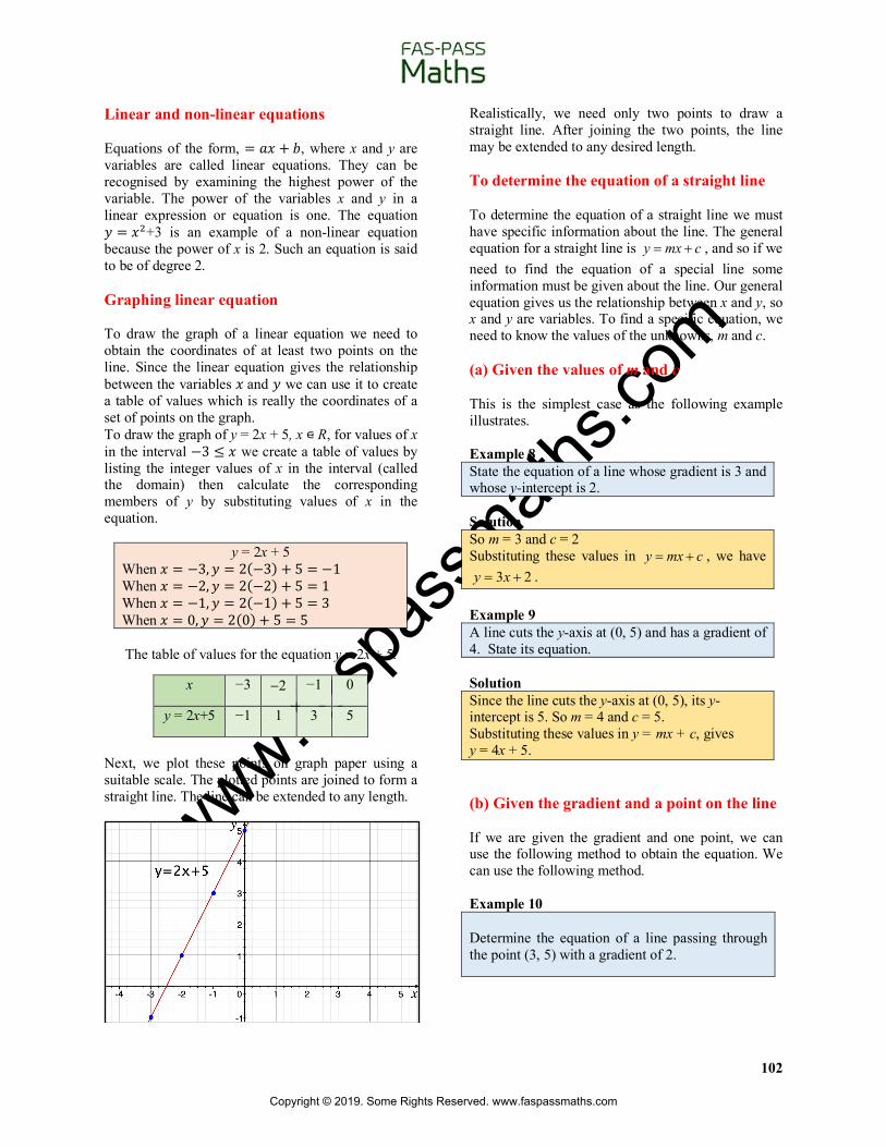
To draw the graph of a linear equation we need to obtain the coordinates of at least two points on the line. Since the linear equation gives the relationship between the variables 𝑥and 𝑦 we can use it to create a table of values which is really the coordinates of a set of points on the graph. To draw the graph of y = 2x + 5, x ⋴ R, for values of x in the interval −3 ≤ 𝑥 we create a table of values by listing the integer values of x in the interval (called the domain) then calculate the corresponding members of y by substituting values of x in the equation.

y = 2x + 5 When 𝑥 = −3, 𝑦 = 2(−3) + 5 = −1 When 𝑥 = −2, 𝑦 = 2(−2) + 5 = 1 When 𝑥 = −1, 𝑦 = 2(−1) + 5 = 3 When 𝑥 = 0, 𝑦 = 2(0) + 5 = 5

The table of values for the equation y = 2x + 5.

x −3 -2 −1 0

y = 2x+5 −1 1 3 5

Next, we plot these points on graph paper using a suitable scale. The plotted points are joined to form a straight line. The line can be extended to any length.

Realistically, we need only two points to draw a straight line. After joining the two points, the line may be extended to any desired length. To determine the equation of a straight line To determine the equation of a straight line we must have specific information about the line. The general equation for a straight line is , and so if we need to find the equation of a special line some information must be given about the line. Our general equation gives us the relationship between x and y, so x and y are variables. To find a specific equation, we need to know the values of the unknowns, m and c. (a) Given the values of m and c This is the simplest case as the following example illustrates. Example 8 State the equation of a line whose gradient is 3 and whose y-intercept is 2. Solution So m = 3 and c = 2 Substituting these values in , we have

. Example 9 A line cuts the y-axis at (0, 5) and has a gradient of 4. State its equation. Solution Since the line cuts the y-axis at (0, 5), its y-intercept is 5. So m = 4 and c = 5. Substituting these values in y = mx + c, gives y = 4x + 5. (b) Given the gradient and a point on the line If we are given the gradient and one point, we can use the following method to obtain the equation. We can use the following method. Example 10 Determine the equation of a line passing through the point (3, 5) with a gradient of 2.

y mx c= +

y mx c= +3 2y x= +


www.fasp

assm

aths.c

om

103

Solution We calculate the value of c by substituting the value of m and the coordinates in the equation

Substituting 𝑚 = 2, 𝑥 = 3𝑎𝑛𝑑𝑦 = 5:

5 = 2(3) + 𝑐 𝑐 = −1

The equation of the line is 𝑦 = 2𝑥 − 1 Alternative method This method relies on a formula, which will now be developed. Let P (x, y) be any point on the line whose gradient is m. Let the given point be A(x1, y1). The gradient of the line is:

This can be re-arranged to

In general, if (x, y) is any point on the line whose gradient is m and the point (x1, y1) lies on the line, the equation of the line is

Example 11 Determine the equation of the line passing through the point (2, 4) and whose gradient is 3.

Solution

The equation is , substituting for m, x1

and y1 , we have

y – 4 = 3 (x – 2) y – 4 = 3 x – 6 (c) Given two points on the line If we are given two points, then we can use the coordinates of the points to calculate the gradient of the line and proceed as we did above. To calculate the gradient we can use the following derived below. Gradient of line joining (x1 , y1 ) to (x2 , y2 )

Example 12 Determine the equation of the line that passes through the points (2, 1) and (4, 7).

y mx c= +

1

1

RiseRuny y mx x-

=-

( )1 1y y m x x- = -

( )1 1y y m x x- = -

1

1

y ymx x-

=-

324=

--xy

3 2y x= -

2 1

2 1

RiseRun

m

y yx x

=

-=

-


www.fasp

assm

aths.c

om

104

Solution The gradient of the line is

Choosing either of the points, say (2, 1),

If we had instead used the point (4, 7) and the same gradient, 3, we would have obtained the same equation. Example 13 Determine the equation of the straight line that passes through O and which is perpendicular to the line with the equation, . Solution The line has gradient 2.

The required line has a gradient

(Using the fact that the product of the gradients of perpendicular lines = − 1) The equation of the required line is

.

Example 14 Find the equation of the line passing through the point (2, −1) and which is parallel to the line with the equation, . Solution

The gradient

The required line has a gradient (parallel

lines have the same gradients) The equation of the required line is

.

Intercepts on the x and y axes To determine the y coordinate on a line which cuts the x – axis, we let y = 0. This is because, at any point where a line cuts the x-axis, the y coordinate is zero. Similarly, to determine the x-coordinate on a line which cuts the y – axis, we let . This is because, at any point where a line cuts the y-axis, the x coordinate is zero. The point where a line cuts the y-axis is called the y-intercept. The point where a line cuts the x-axis is called the x-intercept. Example 15 Determine the coordinates of the points at which the line cuts each axis. Solution

Let

Let

Line cuts the y-axis at (0, -8) and the x-axis at (2, 0). If is sketched, the figure may look like:

2 1

2 1

7 1 6 34 2 2

y ymx x- -

= = = =- -

1

1

132

1 3 63 5

y ymx xyx

y xy x

-=

--

=-

- = -= -

2y x=

2y x=

\ 12

= -

0 1 20 2

y y xx-

= - = --

2 1 0y x+ - =

2 1 01 12 2

y x

y x

+ - =

= - +

\ 12

= -

\ 12

= -

1 1 22 2

y y xx+

= - = --

0x =

4 8y x= -

4 8y x= -0x =

( )4 0 80 88

yyy

= -

= -= -

0y =0 4 84 8

2

xxx

= -==

\

4 8y x= -


12. coordinate geometry...12. coordinate geometry the cartesian plane we recall from our study of...

Documents