12 special relativity - university of new mexico

12

Special relativity

12.1 Inertial frames and Lorentz transformations

An inertial reference frame is a system of coordinates in which freeparticles move in straight lines at constant speeds. Our spacetime has onetime dimension x0 = ct and three space dimensions x. Its physical points arelabeled by four coordinates, p = (x0, x1, x2, x3). The quadratic separationbetween two infinitesimally separated points p and p+dp whose coordinatesdi↵er by dx0, dx1, dx2, dx3 is

ds2 = � c2dt2 + (dx1)2 + (dx2)2 + (dx3)2. (12.1)

In the absence of gravity, ds2 is the physical quadratic separation betweenthe points p and p + dp. Since it is physical, it must not change when wechange coordinates. Changes of coordinates x ! x0 that leave ds2 invariantare called Lorentz transformations.If we adopt the summation convention in which an index is summed

from 0 to 3 if it occurs both raised and lowered in the same monomial, thenwe can write a Lorentz transformation as

x0i =3X

k=0

Lik x

k = Lik x

k. (12.2)

Lorentz transformations change coordinate di↵erences dxk to dx0i = Lik dx

k.The Minkowski-space metric ⌘ik = ⌘ik is the 4⇥ 4 matrix

(⌘ik) =

0

BB@

�1 0 0 00 1 0 00 0 1 00 0 0 1

1

CCA = (⌘ik). (12.3)

It is its own inverse: ⌘2 = I or ⌘ik ⌘k` = �`i .

490 Special relativity

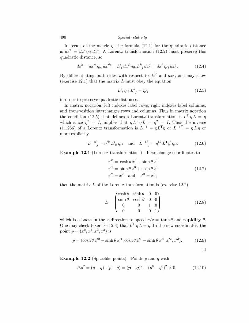
In terms of the metric ⌘, the formula (12.1) for the quadratic distanceis ds2 = dxi ⌘ik dxk. A Lorentz transformation (12.2) must preserve thisquadratic distance, so

ds2 = dx0i ⌘ik dx0k = Li

` dx` ⌘ik L

kj dx

j = dx` ⌘`j dxj . (12.4)

By di↵erentiating both sides with respect to dx` and dxj , one may show(exercise 12.1) that the matrix L must obey the equation

Li` ⌘ik L

kj = ⌘`j (12.5)

in order to preserve quadratic distances.In matrix notation, left indexes label rows; right indexes label columns;

and transposition interchanges rows and columns. Thus in matrix notationthe condition (12.5) that defines a Lorentz transformation is LT ⌘L = ⌘which since ⌘2 = I, implies that ⌘LT ⌘L = ⌘2 = I. Thus the inverse(11.266) of a Lorentz transformation is L�1 = ⌘LT⌘ or L�1T = ⌘L ⌘ ormore explicitly

L�1`j = ⌘`k Li

k ⌘ij and L�1`j = ⌘`k LT i

k ⌘ij . (12.6)

Example 12.1 (Lorentz transformations) If we change coordinates to

x00 = cosh ✓ x0 + sinh ✓ x1

x01 = sinh ✓ x0 + cosh ✓ x1 (12.7)

x02 = x2 and x03 = x3,

then the matrix L of the Lorentz transformation is (exercise 12.2)

L =

0

BB@

cosh ✓ sinh ✓ 0 0sinh ✓ cosh ✓ 0 00 0 1 00 0 0 1

1

CCA (12.8)

which is a boost in the x-direction to speed v/c = tanh ✓ and rapidity ✓.One may check (exercise 12.3) that LT ⌘L = ⌘. In the new coordinates, thepoint p = (x0, x1, x2, x3) is

p = (cosh ✓ x00 � sinh ✓ x01, cosh ✓ x01 � sinh ✓ x00, x02, x03). (12.9)

Example 12.2 (Spacelike points) Points p and q with

�s2 = (p� q) · (p� q) = (p� q)2 � (p0 � q0)2 > 0 (12.10)

12.1 Inertial frames and Lorentz transformations 491

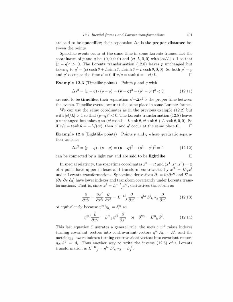
are said to be spacelike; their separation �s is the proper distance be-tween the points.

Spacelike events occur at the same time in some Lorentz frames. Let thecoordinates of p and q be. (0, 0, 0, 0) and (ct, L, 0, 0) with |ct/L| < 1 so that(p � q)2 > 0. The Lorentz transformation (12.8) leaves p unchanged buttakes q to q0 = (ct cosh ✓ + L sinh ✓, ct sinh ✓ + L cosh ✓, 0, 0). So both p0 = pand q0 occur at the time t0 = 0 if v/c = tanh ✓ = �ct/L.

Example 12.3 (Timelike points) Points p and q with

�s2 = (p� q) · (p� q) = (p� q)2 � (p0 � q0)2 < 0 (12.11)

are said to be timelike; their separationp��s2 is the proper time between

the events. Timelike events occur at the same place in some Lorentz frames.We can use the same coordinates as in the previous example (12.2) but

with |ct/L| > 1 so that (p�q)2 < 0. The Lorentz transformation (12.8) leavesp unchanged but takes q to (ct cosh ✓+L sinh ✓, ct sinh ✓+L cosh ✓, 0, 0). Soif v/c = tanh ✓ = �L/(ct), then p0 and q0 occur at the same place 0.

Example 12.4 (Lightlike points) Points p and q whose quadratic separa-tion vanishes

�s2 = (p� q) · (p� q) = (p� q)2 � (p0 � q0)2 = 0 (12.12)

can be connected by a light ray and are said to be lightlike.

In special relativity, the spacetime coordinates x0 = ct and (x1, x2, x3) = x

of a point have upper indexes and transform contravariantly x0k = Lk`x

`

under Lorentz transformations. Spacetime derivatives @0 = @/@x0 and r =(@1, @2, @3) have lower indexes and transform covariantly under Lorentz trans-formations. That is, since x` = L�1`

jx0j , derivatives transform as

@

@x0j=

@x`

@x0j@

@x`= L�1`

j

@

@x`= ⌘`k Li

k ⌘ij@

@x`(12.13)

or equivalently because ⌘mj⌘ij = �mi as

⌘mj @

@x0j= Lm

k ⌘`k @

@x`or @0m = Lm

k @`. (12.14)

This last equation illustrates a general rule: the metric ⌘ik raises indexesturning covariant vectors into contravariant vectors ⌘ik Ak = Ai, and themetric ⌘ik lowers indexes turning contravariant vectors into covariant vectors⌘ik Ak = Ai. Thus another way to write the inverse (12.6) of a Lorentztransformation is L�1`

j = ⌘`k Lik ⌘ij = L `

j .


12.2 Special relativity

The spacetime of special relativity is flat, four-dimensional Minkowski space.In the absence of gravity, the inner product (p� q) · (p� q)

(p� q) · (p� q) = (p� q)2 � (p0 � q0)2 = (p� q)i ⌘ik (p� q)k (12.15)

is physical and the same in all Lorentz frames. If the points p and q are closeneighbors with coordinates xi + dxi for p and xi for q, then that invariantinner product is ds2 = dxi ⌘ij dxj = dx

2 � (dx0)2.If the points p and q are on the trajectory of a massive particle moving

at velocity v, then this invariant quadratic separation

ds2 = dx2 � c2dt2 =

�v2 � c2

�dt2 (12.16)

is negative since v < c. The time in the rest frame of the particle is theproper time ⌧ , and

d⌧2 = � ds2/c2 =�1� v

2/c2�dt2. (12.17)

A particle of mass zero moves at the speed of light, so its element d⌧ ofproper time is zero. But for a particle of mass m > 0 moving at speed v,the element of proper time d⌧ is smaller than the corresponding element oflaboratory time dt by the factor

p1� v2/c2. The proper time is the time

in the rest frame of the particle where v = 0. So if T (0) is the lifetime of aparticle at rest, then the apparent lifetime T (v) when the particle is movingat speed v is

T (v) = dt =d⌧p

1� v2/c2=

T (0)p1� v2/c2

(12.18)

which is longer than T (0) since 1 � v2/c2 1, an e↵ect known as timedilation.

Example 12.5 (Time dilation in muon decay) A muon at rest has a meanlife of T (0) = 2.2⇥ 10�6 seconds. Cosmic rays hitting nitrogen and oxygennuclei make pions high in the Earth’s atmosphere. The pions rapidly decayinto muons in 2.6⇥10�8 s. A muon moving at the speed of light from 10 kmtakes at least t = 10 km/300, 000 (km/sec) = 3.3⇥ 10�5 s to hit the ground.Were it not for time dilation, the probability P of such a muon reaching theground as a muon would be

P = e�t/T (0) = exp(�33/2.2) = e�15 = 2.6⇥ 10�7. (12.19)

12.3 Kinematics 493

The mass of a muon is 105.66 MeV. So a muon of energy E = 749 MeVhas by (12.26) a time-dilation factor of

1p1� v2/c2

=E

mc2=

749

105.7= 7.089 =

1p1� (0.99)2

. (12.20)

So a muon moving at a speed of v = 0.99 c has an apparent mean life T (v)given by equation (12.18) as

T (v) =E

mc2T (0) =

T (0)p1� v2/c2

=2.2⇥ 10�6 sp1� (0.99)2

= 1.6⇥ 10�5 s. (12.21)

The probability of survival with time dilation is

P = e�t/T (v) = exp(�33/16) = 0.12 (12.22)

so that 12% survive. Time dilation increases the chance of survival by afactor of 460,000—no small e↵ect.

12.3 Kinematics

From the scalar d⌧ , and the contravariant vector dxi, we can make the 4-vector

ui =dxi

d⌧=

dt

d⌧

✓dx0

dt,dx

dt

◆=

1p1� v2/c2

(c,v) (12.23)

in which u0 = c dt/d⌧ = c/p1� v2/c2 and u = u0 v/c. The product mui is

the energy-momentum 4-vector pi

pi = mui = mdxi

d⌧= m

dt

d⌧

dxi

dt=

mp1� v2/c2

dxi

dt

=mp

1� v2/c2(c,v) =

✓E

c,p

◆. (12.24)

Its invariant inner product is a constant characteristic of the particle andproportional to the square of its mass

c2 pi pi = mcuimcui = �E2 + c2 p 2 = �m2 c4. (12.25)

Note that the time-dilation factor is the ratio of the energy of a particle toits rest energy

1p1� v2/c2

=E

mc2(12.26)


and the velocity of the particle is its momentum divided by its equivalentmass E/c2

v =p

E/c2. (12.27)

The analog of F = ma is

md2xi

d⌧2= m

dui

d⌧=

dpi

d⌧= f i (12.28)

in which p0 = E/c, and f i is a 4-vector force.

Example 12.6 (Time dilation and proper time) In the frame of a labo-ratory, a particle of mass m with 4-momentum pilab = (E/c, p, 0, 0) travelsa distance L in a time t for a 4-vector displacement of xilab = (ct, L, 0, 0).In its own rest frame, the particle’s 4-momentum and 4-displacement arepirest = (mc, 0, 0, 0) and xirest = (c⌧, 0, 0, 0). Since the Minkowski inner prod-uct of two 4-vectors is Lorentz invariant, we have�pixi

�rest

=�pixi

�lab

or pL�Et = �mc2⌧ = �mc2tp

1� v2/c2. (12.29)

So a massive particle’s phase exp(ipixi/~) is exp(�imc2⌧/~).

Example 12.7 (p + p ! 3p + p) Conservation of the energy-momentum4-vector gives p + p0 = 3p0 + p0. We set c = 1 and use this equality in theinvariant form (p + p0)2 = (3p0 + p0)2. We compute (p + p0)2 = p2 + p20 +2p · p0 = �2m2

p + 2p · p0 in the laboratory frame in which p0 = (m,0). Thus(p+p0)2 = �2m2

p�2Epmp. We compute (3p0+p0)2 in the frame in which eachof the three protons and the antiproton has zero spatial momentum. There(3p0 + p0)2 = (4m,0)2 = �16m2

p. We get Ep = 7mp of which 6mp = 5.63GeV is the threshold kinetic energy of the proton. In 1955, when the groupled by Owen Chamberlain and Emilio Segre discovered the antiproton, thenominal maximum energy of the protons in the Bevatron was 6.2 GeV.

12.4 Electrodynamics

In electrodynamics and in mksa (si) units, the three-dimensional vectorpotential A and the scalar potential � form a covariant 4-vector potential

Ai =

✓��

c,A

◆. (12.30)

12.4 Electrodynamics 495

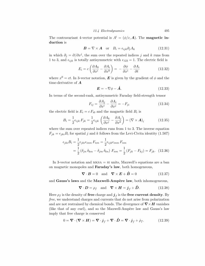
The contravariant 4-vector potential is Ai = (�/c,A). The magnetic in-duction is

B = r⇥A or Bi = ✏ijk@jAk (12.31)

in which @j = @/@xj , the sum over the repeated indices j and k runs from1 to 3, and ✏ijk is totally antisymmetric with ✏123 = 1. The electric field is

Ei = c

✓@A0

@xi� @Ai

@x0

◆= � @�

@xi� @Ai

@t(12.32)

where x0 = ct. In 3-vector notation, E is given by the gradient of � and thetime-derivative of A

E = �r�� A. (12.33)

In terms of the second-rank, antisymmetric Faraday field-strength tensor

Fij =@Aj

@xi� @Ai

@xj= �Fji (12.34)

the electric field is Ei = c Fi0 and the magnetic field Bi is

Bi =1

2✏ijk Fjk =

1

2✏ijk

✓@Ak

@xj� @Aj

@xk

◆= (r⇥A)i (12.35)

where the sum over repeated indices runs from 1 to 3. The inverse equationFjk = ✏jkiBi for spatial j and k follows from the Levi-Civita identity (1.507)

✏jkiBi =1

2✏jki✏inm Fnm =

1

2✏ijk✏inm Fnm

=1

2(�jn �km � �jm �kn) Fnm =

1

2(Fjk � Fkj) = Fjk. (12.36)

In 3-vector notation and mksa = si units, Maxwell’s equations are a banon magnetic monopoles and Faraday’s law, both homogeneous,

r ·B = 0 and r⇥E + B = 0 (12.37)

and Gauss’s laws and the Maxwell-Ampere law, both inhomogeneous,

r ·D = ⇢f and r⇥H = jf + D. (12.38)

Here ⇢f is the density of free charge and jf is the free current density. Byfree, we understand charges and currents that do not arise from polarizationand are not restrained by chemical bonds. The divergence of r⇥H vanishes(like that of any curl), and so the Maxwell-Ampere law and Gauss’s lawimply that free charge is conserved

0 = r · (r⇥H) = r · jf +r · D = r · jf + ⇢f . (12.39)


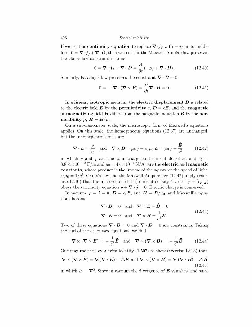
If we use this continuity equation to replace r ·jf with � ⇢f in its middle

form 0 = r ·jf +r ·D, then we see that the Maxwell-Ampere law preservesthe Gauss-law constraint in time

0 = r · jf +r · D =@

@t(�⇢f +r ·D) . (12.40)

Similarly, Faraday’s law preserves the constraint r ·B = 0

0 = �r · (r⇥E) =@

@tr ·B = 0. (12.41)

In a linear, isotropic medium, the electric displacement D is relatedto the electric field E by the permittivity ✏, D = ✏E, and the magneticor magnetizing field H di↵ers from the magnetic induction B by the per-meability µ, H = B/µ.On a sub-nanometer scale, the microscopic form of Maxwell’s equations

applies. On this scale, the homogeneous equations (12.37) are unchanged,but the inhomogeneous ones are

r ·E =⇢

✏0and r⇥B = µ0 j + ✏0 µ0 E = µ0 j +

E

c2(12.42)

in which ⇢ and j are the total charge and current densities, and ✏0 =8.854⇥10�12 F/m and µ0 = 4⇡⇥10�7 N/A2 are the electric and magneticconstants, whose product is the inverse of the square of the speed of light,✏0µ0 = 1/c2. Gauss’s law and the Maxwell-Ampere law (12.42) imply (exer-cise 12.10) that the microscopic (total) current-density 4-vector j = (c⇢, j)obeys the continuity equation ⇢+r · j = 0. Electric charge is conserved.In vacuum, ⇢ = j = 0, D = ✏0E, and H = B/µ0, and Maxwell’s equa-

tions become

r ·B = 0 and r⇥E + B = 0

r ·E = 0 and r⇥B =1

c2E.

(12.43)

Two of these equations r · B = 0 and r · E = 0 are constraints. Takingthe curl of the other two equations, we find

r⇥ (r⇥E) = � 1

c2E and r⇥ (r⇥B) = � 1

c2B. (12.44)

One may use the Levi-Civita identity (1.507) to show (exercise 12.13) that

r⇥ (r⇥E) = r (r · E)�4E and r⇥ (r⇥B) = r (r · B)�4B

(12.45)in which 4 ⌘ r2. Since in vacuum the divergence of E vanishes, and since

12.4 Electrodynamics 497

that ofB always vanishes, these identities and the curl-curl equations (12.44)tell us that waves of E and B move at the speed of light

1

c2E �4E = 0 and

1

c2B �4B = 0. (12.46)

We may write the two homogeneous Maxwell equations (12.37) as

@iFjk + @kFij + @jFki = @i (@jAk � @kAj) + @k (@iAj � @jAi)

+ @j (@kAi � @iAk) = 0 (12.47)

(exercise 12.11). This relation, known as the Bianchi identity, actually isa generally covariant tensor equation

✏`ijk@iFjk = 0 (12.48)

in which ✏`ijk is totally antisymmetric, as explained in Sec. 13.20. There arefour versions of this identity (corresponding to the four ways of choosingthree di↵erent indices i, j, k from among four and leaving out one, `). The` = 0 case gives the scalar equation r · B = 0, and the three that have` 6= 0 give the vector equation r⇥E + B = 0.In tensor notation, the microscopic form of the two inhomogeneous equa-

tions (12.42)—the laws of Gauss and Ampere—are a single equation

@iFki = µ0 j

k in which jk = (c⇢, j) (12.49)

is the current 4-vector.The Lorentz force law for a particle of charge q is

md2xi

d⌧2= m

dui

d⌧=

dpi

d⌧= f i = q F ij dxj

d⌧= q F ij uj . (12.50)

We may cancel a factor of dt/d⌧ from both sides and find for i = 1, 2, 3

dpi

dt= q

��F i0 + ✏ijkBkvj

�or

dp

dt= q (E + v ⇥B) (12.51)

and for i = 0dE

dt= qE · v (12.52)

which shows that only the electric field does work. The only special-relativisticcorrection needed in Maxwell’s electrodynamics is a factor of 1/

p1� v2/c2

in these equations. That is, we use p = mu = mv/p1� v2/c2 not p = mv

in (12.51), and we use the total energy E not the kinetic energy in (12.52).The reason why so little of classical electrodynamics was changed by specialrelativity is that electric and magnetic e↵ects were accessible to measure-ment during the 1800’s. Classical electrodynamics was almost perfect.


Keeping track of factors of the speed of light is a lot of trouble and adistraction; in what follows, we’ll often use units with c = 1.

12.5 Principle of stationary action in special relativity

The action for a free particle of mass m in special relativity is

S = �m

Z ⌧2

⌧1

d⌧ = �Z t2

t1

mp1� x

2 dt (12.53)

where c = 1 and x = dx/dt. The requirement of stationary action is

0 = �S = � �

Z t2

t1

mp1� x

2 dt = m

Z t2

t1

x · �xp1� x

2dt. (12.54)

But 1/p

1� x2 = dt/d⌧ and so

0 = �S = m

Z t2

t1

dx

dt· d�xdt

dt

d⌧dt = m

Z ⌧2

⌧1

dx

dt· d�xdt

dt

d⌧

dt

d⌧d⌧

= m

Z ⌧2

⌧1

dx

d⌧· d�xd⌧

d⌧. (12.55)

So integrating by parts, keeping in mind that �x(⌧2) = �x(⌧1) = 0, we have

0 = �S = m

Z ⌧2

⌧1

d

d⌧

✓dx

d⌧· �x

◆� d2x

d⌧2· �x

�d⌧ = �m

Z ⌧2

⌧1

d2x

d⌧2· �x d⌧.

(12.56)To have this hold for arbitrary �x, we need

d2x

d⌧2= 0 (12.57)

which is the equation of motion for a free particle in special relativity.What about a charged particle in an electromagnetic field Ai? Its action

is

S = �m

Z ⌧2

⌧1

d⌧ + q

Z x2

x1

Ai(x) dxi =

Z ⌧2

⌧1

✓�m+ qAi(x)

dxi

d⌧

◆d⌧. (12.58)

We now treat the first term in a four-dimensional manner

�d⌧ = �p�⌘ikdxidxk =

�⌘ikdxi�dxkp�⌘ikdxidxk

= �uk�dxk = �ukd�x

k (12.59)

12.6 Di↵erential forms 499

in which uk = dxk/d⌧ is the 4-velocity (12.23) and ⌘ is the Minkowski metric(12.3) of flat spacetime. The variation of the other term is

��Ai dx

i�= (�Ai) dx

i +Ai �dxi = Ai,k�x

k dxi +Ai d�xi. (12.60)

Putting them together, we get for �S

�S =

Z ⌧2

⌧1

✓muk

d�xk

d⌧+ qAi,k�x

k dxi

d⌧+ qAi

d�xi

d⌧

◆d⌧. (12.61)

After integrating by parts the last term, dropping the boundary terms, andchanging a dummy index, we get

�S =

Z ⌧2

⌧1

✓�m

dukd⌧

�xk + qAi,k�xk dx

i

d⌧� q

dAk

d⌧�xk

◆d⌧

=

Z ⌧2

⌧1

�m

dukd⌧

+ q�Ai,k �Ak,i

� dxi

d⌧

��xk d⌧. (12.62)

If this first-order variation of the action is to vanish for arbitrary �xk, thenthe particle must follow the path

0 = �mdukd⌧

+ q�Ai,k �Ak,i

� dxi

d⌧or

dpk

d⌧= qF kiui (12.63)

which is the Lorentz force law (12.50).

12.6 Di↵erential forms

By (13.9 & 13.4), a covariant vector field contracted with contravariant co-ordinate di↵erentials is invariant under arbitrary coordinate transformations

A0 = A0i dx

0i =@xj

@x0iAj

@x0i

@xkdxk = �jk Aj dx

k = Ak dxk = A. (12.64)

This invariant quantity A = Ak dxk is a called a 1-form in the language ofdi↵erential forms introduced about a century ago by Elie Cartan, son ofa blacksmith (1869–1951).

The wedge product dx^dy of two coordinate di↵erentials is the directedarea spanned by the two di↵erentials and is defined to be antisymmetric

dx ^ dy = � dy ^ dx and dx ^ dx = dy ^ dy = 0 (12.65)

so as to transform correctly under a change of coordinates. In terms of thecoordinates u = u(x, y) and v = v(x, y), the new element of area is

du ^ dv =

✓@u

@xdx+

@u

@ydy

◆^✓@v

@xdx+

@v

@ydy

◆. (12.66)


Labeling partial derivatives by subscripts (2.7) and using the antisymmetry(12.65) of the wedge product, we see that du ^ dv is the old area dx ^ dymultiplied by the Jacobian (section 1.22) of the transformation x, y ! u, v

du ^ dv = (uxdx+ uydy) ^ (vxdx+ vydy)

= ux vx dx ^ dx+ ux vy dx ^ dy + uy vx dy ^ dx+ uy vy dy ^ dy

= (ux vy � uyvx) dx ^ dy

=

��ux uyvx vy

�� dx ^ dy = J(u, v;x, y) dx ^ dy. (12.67)

A contraction H = 12Hik dxi ^ dxk of a second-rank covariant tensor with

a wedge product of two di↵erentials is a 2-form. A p -form is a rank-pcovariant tensor contracted with a wedge product of p di↵erentials

K =1

p!Ki1...ip dx

i1 ^ . . . dxip . (12.68)

The exterior derivative d di↵erentiates and adds a di↵erential. It turnsa p-form into a (p+ 1)-form. It turns a function f , which is a 0-form, intoa 1-form

df =@f

@xidxi (12.69)

and a 1-form A = Aj dxj into a 2-form dA = d(Aj dxj)= (@iAj) dxi ^ dxj .

Example 12.8 (The Curl) The exterior derivative of the 1-form

A = Ax dx+Ay dy +Az dz (12.70)

is a 2-form that contains the curl (2.42) of A

dA = @yAx dy ^ dx+ @zAx dz ^ dx

+ @xAy dx ^ dy + @zAy dz ^ dy

+ @xAz dx ^ dz + @yAz dy ^ dz

= (@yAz � @zAy) dy ^ dz (12.71)

+ (@zAx � @xAz) dz ^ dx

+ (@xAy � @yAx) dx ^ dy

= (r⇥A)x dy ^ dz + (r⇥A)y dz ^ dx+ (r⇥A)z dx ^ dy.

The exterior derivative of the electromagnetic 1-form A = Aj dxj made

12.6 Di↵erential forms 501

from the 4-vector potential or gauge field Aj is the Faraday 2-form (12.34),the tensor Fij

dA = d�Aj dx

j�= @iAj dx

i ^ dxj = 12 Fij dx

i ^ dxj = F (12.72)

in which @i = @/@xi.The square dd of the exterior derivative vanishes in the sense that dd

applied to any p-form Q is zero

d⇥d�Qi...dx

i ^ . . .�⇤

= d⇥(@rQi...) dx

r ^ dxi ^ . . .⇤

= (@s@rQi...) dxs ^ dxr ^ dxi ^ . . . = 0

(12.73)

because @s@rQ is symmetric in r and s while dxs ^ dxr is anti-symmetric.If Mik is a covariant second-rank tensor with no particular symmetry,

then (exercise 12.12) only its antisymmetric part contributes to the 2-formMik dxi ^ dxk and only its symmetric part contributes to Mik dxidxk.

Example 12.9 (The homogeneous Maxwell equations) The exterior deriva-tive d applied to the Faraday 2-form F = dA gives the homogeneous Maxwellequations

0 = ddA = dF = dFik dxi ^ dxk = @`Fik dx

` ^ dxi ^ dxk (12.74)

an equation known as the Bianchi identity (12.48).

A p-form H is closed if dH = 0. By (12.74), the Faraday 2-form is closed,dF = 0. A p-form H is exact if it is the di↵erential H = dK of a (p � 1)-form K. The identity (12.73) or dd = 0 implies that every exact form isclosed. A lemma (section 14.5) due to Poincare shows that every closedform is locally exact.

If the Ai in the 1-form A = Aidxi commute with each other, then the 2-form A^A is identically zero. But if the Ai don’t commute because they arematrices, operators, or Grassmann variables, then A^A = 1

2 [Ai, Aj ] dxi^dxjneed not vanish.

Example 12.10 (If B = 0, the electric field is closed and exact) If B = 0,then by Faraday’s law (12.37) the curl of the electric field vanishes,r ⇥ E =0. In terms of the 1-form E = Ei dxi for i = 1, 2, 3, the vanishing of its curlr ⇥ E is

dE = @jEi dxj ^ dxi =

1

2(@jEi � @iEj) dx

j ^ dxi = 0. (12.75)

So E is closed. It also is exact because we can define a quantity V (x) whose


gradient is E = �rV . We first define VP (x) as a line integral of the 1-formE along an arbitrary path P from some starting point x0 to x

VP (x) = �Z x

P,x0

Ei dxi = �

Z

PE. (12.76)

The potential VP (x) might seem to depend on the path P . But the di↵erenceVP 0(x) � VP (x) is a line integral of E from x0 to x along the path P 0 andthen back to x0 along the path P . And by Stokes’s theorem (2.50), theintegral of E around such a closed loop is an integral of the curl r ⇥ E ofE over any surface S whose boundary is that closed loop.

VP 0(x)� VP (x) =

I

P�P 0Ei dx

i =

Z

S(r ⇥ E) · da = 0. (12.77)

In the notation of forms, this is

VP 0(x)� VP (x) =

Z

@SE =

Z

SdE = 0. (12.78)

Thus the potential VP (x) = V (x) is independent of the path, and E =�rV (x), and so the 1-form E = Ei dxi = �@iV dxi = �dV is exact.

The general form of Stokes’s theorem is that the integral of any p-formH over the boundary @R of any (p + 1)-dimensional, simply connected,orientable region R is equal to the integral of the (p+ 1)-form dH over R

Z

@RH =

Z

RdH. (12.79)

Equation (12.78) is the p = 1 case (George Stokes, 1819–1903).

Example 12.11 (Stokes’s theorem for 0-forms) When p = 0, the regionR = [a, b] is 1-dimensional, H is a 0-form, and Stokes’s theorem is theformula of elementary calculus

H(b)�H(a) =

Z

@RH =

Z

RdH =

Z b

adH(x) =

Z b

aH 0(x) dx. (12.80)

Example 12.12 (Exterior derivatives anticommute with di↵erentials) Theexterior derivative acting on the wedge product of two 1-forms A = Aidxi

Exercises 503

and B = B`dx` is

d(A ^B) = d(Aidxi ^B`dx

`) = @k(AiB`) dxk ^ dxi ^ dx` (12.81)

= (@kAi)B` dxk ^ dxi ^ dx` +Ai (@kB`) dx

k ^ dxi ^ dx`

= (@kAi)B` dxk ^ dxi ^ dx` �Ai (@kB`) dx

i ^ dxk ^ dx`

= (@kAi) dxk ^ dxi ^B`dx

` �Aidxi ^ (@kB`) dx

k ^ dx`

= dA ^B �A ^ dB.

If A is a p-form, then d(A^B) = dA^B+(�1)pA^dB (exercise 12.14).

Although I have avoided gravity in this chapter, special relativity is notin conflict with general relativity. In fact, Einstein’s equivalence principlesays that special relativity applies in a suitably small neighborhood of anypoint in any inertial reference frame that has free-fall coordinates.

Exercises

12.1 Show that (12.4) implies (12.5).

12.2 Show that the matrix form of the Lorentz transformation (12.7) is thex boost (12.8).

12.3 Show that the Lorentz matrix (12.8) satisfies LT ⌘L = ⌘.

12.4 The basis vectors at a point p are the derivatives of the point withrespect to the coordinates. Find the basis vectors ei = @p/@xi at thepoint p = (x0, x1, x2, x3). What are the basis vectors e0i in the coordi-nates x0 (12.9)?

12.5 The basis vectors ei that are dual to the basis vectors ek are definedby ei = ⌘ik ek. (a) Show that they obey ei · ek = �ik. (b) In the twocoordinate systems described in example 12.1, the vectors ek xk ande0i x

0i represent the same point, so ek xk = e0i x0i. Find a formula for

e0i · ek. (c) Relate e0i · ek to the Lorentz matrix (12.8).

12.6 Show that the equality of the inner products xi⌘ikxk = x0j⌘j`x0` meansthat the matrix Li

k = e0i · ek that relates the coordinates x0i = Lik x

k

to the coordinates xk must obey the relation ⌘ik = Lik ⌘i` L

`k which

is ⌘ = LT⌘L in matrix notation. Hint: First doubly di↵erentiate theequality with respect to xk and to x` for k 6= `. Then di↵erentiate ittwice with respect to xk.

12.7 The relations x0i = e0i · ej xj and x` = e` · e0k xk imply (for fixed basis


vectors e and e0) that

@x0i

@xj= e0i · ej = ej · e0i = ⌘j` ⌘

ike` · e0k = ⌘j` ⌘ik @x`

@x0k.

Use this equation to show that if Ai transforms (13.6) as a contravariantvector

A0i =

@x0i

@xjAj , (12.82)

then A` = ⌘`j Aj transforms covariantly (13.9)

A0s =

@x`

@x0sA`.

The metric ⌘ also turns a covariant vector A` into its contravariantform ⌘k`A` = ⌘k`⌘`jAj = �kjA

j = Ak.12.8 The LHC is designed to collide 7 TeV protons against 7 TeV protons for

a total collision energy of 14 TeV. Suppose one used a linear acceleratorto fire a beam of protons at a target of protons at rest at one end ofthe accelerator. What energy would you need to see the same physicsas at the LHC?

12.9 What is the minimum energy that a beam of pions must have to pro-duce a sigma hyperon and a kaon by striking a proton at rest? The rel-evant masses (in MeV) are m⌃+ = 1189.4, mK+ = 493.7, mp = 938.3,and m⇡+ = 139.6.

12.10 Use Gauss’s law and the Maxwell-Ampere law (12.42) to show thatthe microscopic (total) current-density 4-vector j = (c⇢, j) obeys thecontinuity equation ⇢+r · j = 0.

12.11 Derive the Bianchi identity (12.47) from the definition (12.34) of theFaraday field-strength tensor, and show that it implies the two homo-geneous Maxwell equations (12.37).

12.12 Show that if Mik is a covariant second-rank tensor with no particularsymmetry, then only its antisymmetric part contributes to the 2-formMik dxi ^ dxk and only its symmetric part contributes to the quantityMik dxidxk.

12.13 In rectangular coordinates, use the Levi-Civita identity (1.507) toderive the curl-curl equations (12.45).

12.14 Show that if A is a p-form, then d(AB) = dA ^B + (�1)pA ^ dB.12.15 Show that if ! = aijdxi ^ dxj/2 with aij = � aji, then

d! =1

3!(@kaij + @iajk + @jaki) dx

i ^ dxj ^ dxk. (12.83)

12 special relativity - university of new mexico

Documents