1.2 the bayesian case
TRANSCRIPT
Aggregation of Multiple Prior Opinions∗
Hervé Crès†, Itzhak Gilboa‡, and Nicolas Vieille§
Revised, October 2010
Abstract
Experts are asked to provide their advice in a situation of uncer-tainty. They adopt the decision maker’s utility function, but each hasa set of prior probabilities, and so does the decision maker. The de-cision maker and the experts maximize the minimal expected utilitywith respect to their sets of priors. We show that a natural Paretocondition is equivalent to the existence of a set Λ of probability vectorsover the experts, interpreted as possible allocations of weights to theexperts, such that (i) the decision maker’s set of priors is precisely allthe weighted-averages of priors, where an expert’s prior is taken fromher set and the weight vector is taken from Λ; (ii) the decision maker’svaluation of an act is the minimal weighted valuation, over all weightvectors in Λ, of the experts’ valuations.
1 Introduction
1.1 The problem
A decision maker is offered a partnership in a business venture. The offer
appears very attractive, but, after she talks to some friends, it’s pointed out
∗We thank Thibault Gajdos, Philippe Mongin, Ben Polak, Jean-Christophe Vergnaud,four anonymous reviewers, and the associate editor for many detailed comments and ref-erences.
†Sciences-Po, Paris. [email protected]‡HEC, Paris, and Tel-Aviv University, [email protected]§HEC, Paris. [email protected]
1
to her that the project will be a serious failure if the globe becomes warmer
by 3-4 degrees Celsius. She decides to study the matter and to find out what,
according to the experts, is the probability of such a warming taking place
within, say, the next ten years.
It turns out that different experts have different opinions. Indeed, the
phenomenon of global warming that we presumably witness today is not
similar enough to anything that we have observed in the past. The cycles of
the globe’s temperature take a very long time, and the conditions that pre-
vailed in past warmings differ significantly from those in the present. Thus,
one cannot resort to simple empirical frequencies in order to assess probabil-
ities. More sophisticated econometric techniques should be invoked to come
up with such assessments, but they tend to depend on assumptions that are
not shared by all. In short, the experts do not agree, and we cannot assume
that the event in question has an “objective” probability. What should the
decision maker do? What is a rational way of aggregating the opinions of
the experts?
1.2 The Bayesian case
Consider first the benchmark case in which all experts are Bayesian. Specif-
ically, let pi be the subjective probability of the event according to expert
i = 1, ..., n. It seems very natural to take the arithmetic average of the as-
sessments of the experts. This approach may be a little too simple because
it treats all experts equally. More generally, we may consider a weighted
average of the experts’ opinions. For every vector of non-negative weights
λ = (λi)i summing up to 1, we may define
p0 = pλ0 =nXi=1
λipi (1)
Moreover, in a more general case where pi are probability vectors, distribu-
tions on the real line, or general probability measures, their weighted average
2
pλ0 is well-defined, and suggests itself as a natural candidate for the deci-
sion maker’s beliefs. This rule for aggregation of probabilistic assessments
has been dubbed linear opinion pool by Stone (1961), and is attributed to
Laplace (see Bacharach, 1979, McConway, 1981, and Genest and Zidek, 1986,
for a survey).
We will henceforth interpret p0, p1, ..., pn as probability measures on a
state space, and refer to
p0(A) = pλ0(A) =nXi=1
λipi(A)
when we discuss the probability of a specific event A.
The weight λi can be viewed as the degree of confidence the decision maker
has in expert i. Another interpretation is the following: suppose that there
exists an “objective” uncertainty about the state that will obtain, and the
“true” probability is known to be one of p1, ..., pn. The decision maker knows
this structure, but does not know which of p1, ..., pn is the actual probability,
or the “real” data generating process. If the decision maker has Bayesian
beliefs over the objective probability, given by the weights λ = (λi)i, then
p0 is her derived subjective probability over the state space. Thus, we can
think of the decision maker as if she believed that one expert is guaranteed
to generate the “correct” probability, and attaching the probability λi to
the event that expert i has access to “the truth”. We will refer to this
interpretation as “the truth metaphor”.1
The averaging of probabilities resembles the averaging of utilities in social
choice theory. Correspondingly, such an averaging can be derived from a
Pareto, or a unanimity condition à la Harsanyi (1955). Specifically, the
decision maker’s probability p0 is of the form (1) if and only if the following
holds: for every two choices a and b, and every utility function u, if all experts
agree that the expected utility (u) of a is at least as high as that of b, so
1We find this interpretation useful, but it should be stressed that our model does notcapture notions such as “truth” or “objectivity”.
3

should the decision maker.2
1.3 Uncertainty with Bayesian experts
In terms of elegance and internal coherence, the Bayesian paradigm is hardly
matched by any other approach to modeling uncertainty. Moreover, it relies
on powerful axiomatic foundations laid by Ramsey (1931), de Finetti (1931,
1937), and Savage (1954). Yet, it has been criticized on descriptive and nor-
mative grounds alike. Following the seminal contributions of Knight (1921),
Ellsberg (1961), and Schmeidler (1986, 1989), there is a growing body of
literature dealing with more general models representing uncertainty.3 Im-
portantly, many authors view these models as not necessarily less rational
than the Bayesian benchmark. In particular, since the Bayesian approach
calls for the formulation of subjective beliefs, it has been argued that the
very fact that these beliefs differ across individuals might indicate that it is
perhaps not rational to insist on one of them.4 In our context, the decision
maker may ask herself, “If the experts fail to agree on the probability, how
can I be so sure that there is one probability that is ‘correct’? Maybe it’s
safer to allow for a set of possible probabilities, rather than pick only one?”
In this paper we focus on the maxmin expected utility (“MEU”) model,
suggested by Gilboa and Schmeidler (GS 1989), which is arguably the sim-
plest multiple prior model that defines a complete ordering over alternatives.5
2Such derivations are restricted to the case in which all experts share the same utilityfunction, and they require some richness conditions. Hylland and Zeckhauser (1979),Mongin (1995), Blackorby, Donaldson, and Mongin (2004), Chambers and Hayashi (2006)and Zuber (2009) provided impossibility results for the simultaneous aggregation of utilitiesand probabilities. Gilboa, Samet, and Schmeidler (2004) restricted unanimity to choicesover which there are no differences of belief, and derived condition (1) under certainassumptions. However, Gajdos, Tallon, and Vergnaud (2008) showed that in the presenceof uncertainty aggregation of preferences is impossible even if the agents have the samebeliefs.
3See Gilboa (2009) and Gilboa and Marinacci (2010) for surveys of axiomatic founda-tions of the Bayesian approach, their critiques, and alternative models.
4See Gilboa, Postlewaite, and Schmeidler, 2008, 2009, 2010.5Sets of probabilities that are used to define incomplete preferences were studied by
4

Given a set of probabilities C, each possible act f is evaluated by
J(f) = minp∈C
EUp(f)
where EUp(f) is the expected utility of act f according to the probability
p. Uncertainty aversion is built into this decision rule by the min operator,
evaluating each act by its worst-case expected utility (over p ∈ C).
Applied to our context, the decision maker may, for example, be very
cautious and consider as the set C all the probability assessments of the
experts, or, equivalently, their convex hull. This may be a little extreme,
however. If, for example, nine experts evaluate P (A) at 0.4 and one at 0.1,
the range of probabilities for the event A will be [0.1, 0.4]. Clearly, the same
interval would result from nine experts providing the assessment P (A) = 0.1
and only one the assessment 0.4. Consequently, the decision maker may
adopt a set of probabilities that is strictly smaller than the entire convex hull
of the experts’ beliefs. For instance, the decision maker may consider
C =
(p =
nXi=1
λipi |(λ1, ..., λn) ∈ Λ
)
where Λ ⊂ ∆({1, ..., n}) is a set of weight vectors over the n experts. If Λ isa singleton, Λ = (λ1, ..., λn), the decision maker’s behavior will be Bayesian,
with the probability given by (1). If, by contrast, Λ = ∆({1, ..., n}), so thatthe decision maker allows for any possible vector of weights on the experts’
opinions, the decision maker will behave according to the MEU model, with
extreme uncertainty aversion as discussed above. In between these extremes,
a non-singleton, proper subset Λ of ∆({1, ..., n}) allows the decision makerto (i) assign different weights to different experts; (ii) take into account how
many experts provided a certain assessment; and (iii) leave room for a healthy
degree of doubt.
Bewley (2002).
5

1.4 Uncertainty averse experts
If, however, we accept the possibility that rationality, or at least scientific
caution, may favor a set of probabilities over a single one, then we should also
allow the experts to provide their assessments by sets, rather than by single,
probabilities. Indeed, if the experts use standard statistical techniques, they
may come up with confidence sets that cannot be shrunk to singletons with-
out compromising the notion of “confidence”. Thus we re-phrase the question
and ask, how can beliefs be aggregated, where “beliefs” are modeled by sets
of probabilities?
The procedure suggested above consisted in representing beliefs by a class
of weighted averages of experts’ beliefs, with varying weight vectors. It has a
natural extension to the case of non-Bayesian experts: let Λ ⊂ ∆({1, ..., n})be a set of weight vectors over the experts. Assume that each expert has
beliefs that are modeled as a set of probabilities Ci. Then, let the decision
maker entertain the beliefs given by the set
C0 =
(p =
nXi=1
λipi |λ ∈ Λ, pi ∈ Ci
). (2)
Assume that the decision maker uses this set in the context of the maxmin
expected utility model. As in the case in which Ci are singletons, this formula
allows the decision maker a wide range of attitudes towards the experts’
opinions. If Λ is a singleton, the decision maker does not add any uncertainty
aversion of her own: she takes a fixed average of all probabilities the experts
deem possible, and the freedom of choosing a probability in C0 is entirely due
to the fact that the experts fail to commit to a single probability measure. By
contrast, if Λ is the entire simplex∆({1, ..., n}), the decision maker behaves asif any probability that at least one expert deems possible is indeed possible.
And different sets Λ between these extremes allow for different attitudes
towards the uncertainty generated by the choice of the expert.
One attractive feature of the decision rule proposed here is the follow-
6
ing. Assume that each expert i uses the maxmin EU principle with a set of
probabilities Ci as above. Given an act f , expert i evaluates it by
Ji(f) = minp∈Ci
EUp(f)
Suppose that the experts do not report their entire sets of beliefs Ci, but
only their bottom-line evaluation Ji(f). Using the “truth metaphor”, the
decision maker then faces uncertainty about which expert is closest to the
“truth”. As above, the decision maker may consider n epistemic states of
nature, where in state i expert i is right. Thus, if the decision maker knew
which of the experts had access to “truth”, she would follow that expert and
evaluate f by Ji(f). However, the decision maker does not know which expert
has the correct assessment. Facing this uncertainty, the decision maker might
adopt the maxmin EU rule, with a set of probabilities Λ ⊂ ∆({1, ..., n}). Thedecision maker should therefore evaluate act f by
J0(f) = minλ∈Λ
nXi=1
λiJi(f). (3)
It turns out that this evaluation coincides with the rule proposed above
for the same set Λ.6 In other words, if the decision maker had access to
the probabilities used by each expert, Ci, and were she to use the MEU rule
relative to the set C0 given in (2), she would have arrived at precisely the
same conclusion as she would if she followed the rule (3) for the same set
Λ. Thus, the set of weight vectors over the experts, Λ, can be interpreted
in two equivalent ways, as in the Bayesian case: as a set of weights used to
average the experts’ beliefs, and as a set of probabilities over which expert
is “right”. In particular, the decision maker can use the rule (3), applying
to the bottom-line evaluations of the experts, knowing that she would have
arrived at the same evaluation had she asked the experts for their entire sets
of probabilities.
6This fact, which is rather straightforward, is formally stated and proved in the sequel.
7

Gajdos and Vergnaud (2009) also deal with the aggregation of expert
opinions under uncertainty. While their approach differs from ours in several
significant ways (to be discussed below), they also axiomatize a functional of
the form (3).
The MEU model has been criticized for its inability to disentangle objec-
tive, given uncertainty, which is presumably a feature of the decision problem
at hand, from the subjective taste for uncertainty, which is a trait of the deci-
sion maker. For example, if we observe a set C that is a singleton, we cannot
tell whether the decision maker has very precise information about the prob-
lem, allowing her to formulate a Bayesian prior, or has a natural tendency
to treat uncertain situations as if they were risky. Gajdos, Hayashi, Tallon,
and Vergnaud (2008) explicitly model both “hard” information and the set
of priors that governs behavior, allowing for the latter to be a proper subset
of the former.7
In our context, we interpret the sets Ci of the experts as their objec-
tive information, ignoring whatever attitudes towards uncertainty they may
have. By contrast, the set Λ may reflect both the decision maker’s informa-
tion about the experts’ reliability and experience, and her attitude towards
uncertainty. Thus, it is possible that, given the same expert advice and the
same information about the experts, a certain decision maker will choose a
larger set Λ than will another decision maker, who is less averse to uncer-
tainty.
The remainder of the paper is organized as follows. We first define the
formal framework in subsection 2.1. The aggregation rule discussed above is
formally stated in subsection 2.2, where we also state the equivalence between
applying the MEU approach to the experts’ valuations and applying it to the
original problem, with the convex combinations of the experts’ probabilities.
7Another approach to separate uncertainty from uncertainty attitudes is the “smooth”model (Klibanoff, Marinacci, Mukerji, 2005, Nau, 2006, and Seo, 2009), where the decisionmaker is assumed to aggregate (in a non-linear way) various expected utility evaluationsof an act rather than focus on the minimal one.
8

We then turn to axiomatize this rule. To this end, we first explain the
axiomatization informally in subsection 2.3. Finally, the main result is stated
in subsection 2.4 and proved in the Appendix. Section 3 concludes with a
discussion of related literature.
2 Model and Results
2.1 Set-Up
We use a version of the Anscombe-Aumann (AA, 1963) model as re-stated
by Fishburn (1970).
Let X be a set of outcomes. Let L denote the set of von Neumann-
Morgenstern (vNM, 1944) lotteries, that is, the distributions onX with finite
support. L is endowed with a mixing operation: for every P,Q ∈ L and every
α ∈ [0, 1], αP + (1− α)Q ∈ L is given by
(αP + (1− α)Q) (x) = αP (x) + (1− α)Q(x).
The set of states of the world is S and it is endowed with a σ-algebra of
events Σ. The set of acts, F , consists of the Σ-measurable simple functions
from S to L. It is endowed with a mixture operation as well, performed
pointwise. That is, for every f, g ∈ F and every α ∈ [0, 1], αf +(1−α)g ∈ F
is given by
(αf + (1− α)g) (s) = αf(s) + (1− α)g(s).
The decision maker (i = 0) and n experts (i = 1, ..., n) have binary
relations %i⊂ F×F , interpreted as preference relations. The relations Âi,∼i
are defined as usual, namely, as the asymmetric and symmetric parts of %i,
respectively.
We extend the relations (%i)i to L as usual. Thus, for P,Q ∈ L, P %i Q
means fP %i fQ where, for every R ∈ L, fR ∈ F is the constant act given by
fR(s) = R for all s ∈ S. The set of all constant acts is denoted Fc.
9
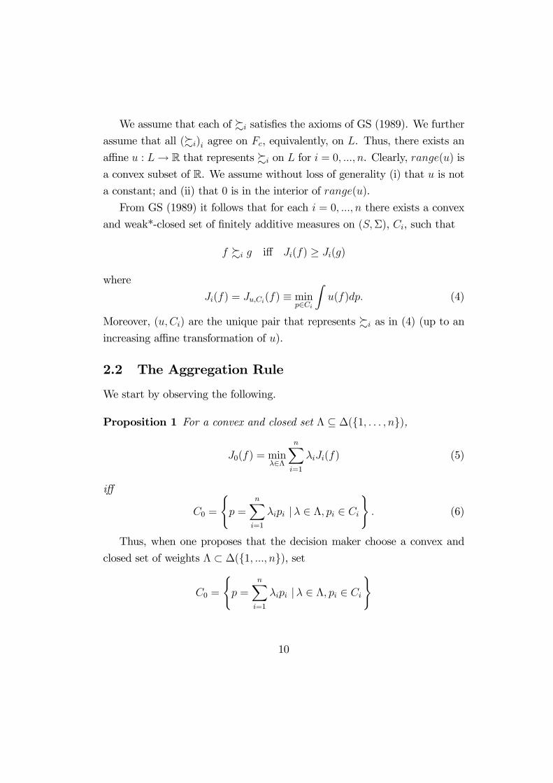
We assume that each of %i satisfies the axioms of GS (1989). We further
assume that all (%i)i agree on Fc, equivalently, on L. Thus, there exists an
affine u : L→ R that represents %i on L for i = 0, ..., n. Clearly, range(u) is
a convex subset of R. We assume without loss of generality (i) that u is nota constant; and (ii) that 0 is in the interior of range(u).
From GS (1989) it follows that for each i = 0, ..., n there exists a convex
and weak*-closed set of finitely additive measures on (S,Σ), Ci, such that
f %i g iff Ji(f) ≥ Ji(g)
where
Ji(f) = Ju,Ci(f) ≡ minp∈Ci
Zu(f)dp. (4)
Moreover, (u,Ci) are the unique pair that represents %i as in (4) (up to an
increasing affine transformation of u).
2.2 The Aggregation Rule
We start by observing the following.
Proposition 1 For a convex and closed set Λ ⊆ ∆({1, . . . , n}),
J0(f) = minλ∈Λ
nXi=1
λiJi(f) (5)
iff
C0 =
(p =
nXi=1
λipi |λ ∈ Λ, pi ∈ Ci
). (6)
Thus, when one proposes that the decision maker choose a convex and
closed set of weights Λ ⊂ ∆({1, ..., n}), set
C0 =
(p =
nXi=1
λipi |λ ∈ Λ, pi ∈ Ci
)
10
and then define, as above,
J0(f) = minp∈C0
Zu(f)dp,
one may equivalently propose that the decision maker employ the MEU
approach on the experts’ valuations, using the same set of weights Λ ⊂∆({1, ..., n}).
2.3 Motivating the Axiomatization
In the Bayesian setting the averaging over the experts’ opinions follows from a
unanimity principle. As in Harsanyi’s (1955) result, if all preference function-
als are linear, then, under certain richness conditions, unanimity implies that
the functional representing society’s preferences is a linear combination of the
functionals representing individuals’ preferences. But in a non-Bayesian set-
ting, this is no longer the case. Unanimity implies (i) that society’s functional
can be written as a function of the functionals of the individuals; and (ii)
that this function is non-decreasing. Assuming that all functionals are con-
tinuous, one may conclude that there exists a continuous and non-decreasing
function ϕ such that, for every act f ,
J0(f) = ϕ (J1(f), ..., Jn(f)) (7)
where ϕ is defined over the range of the Ji’s.
To derive a representation as in (3), one needs to know more about the
function ϕ. First, it has to satisfy (1-)homogeneity and Shift whenever de-
fined:
(i) ϕ is homogenous if for a = (a1, ..., an) ∈ Rn, γ > 0,
ϕ(γa) = γϕ(a)
(i) ϕ satisfies Shift if for a = (a1, ..., an) ∈ Rn, and c ∈ R,
ϕ(a+−→c ) = ϕ(a) + c
11

where −→c = (c, ..., c) ∈ Rn.
Second, ϕ has to be concave.
The fact that J0, J1, ..., Jn are all MEU functionals implies that each of
them satisfies the corresponding properties, appropriately formulated for the
space of acts. It turns out that this is sufficient to determine that ϕ satisfies
homogeneity and Shift. Intuitively, this is similar to arguing that if ϕ maps
linear functionals into a linear functional, ϕ itself has to be linear. However,
concavity does not have this property: even in the case n = 1 the fact that
a functional J is concave and that ϕ(J) is concave does not imply that ϕ is
concave.
One may, of course, stop here, and consider functionals as in (7) where ϕ
need not be concave, rather than insist on the MEU-style aggregation of the
experts’ evaluations. However, the following example illustrates why we find
concavity of ϕ natural in this setting.
Let there be two states 1, 2 and two experts. Expert 1 believes that state
1 is at least as likely as state 2, while expert 2 believes that state 2 is at
least as likely as state 1. That is, C1 = {p ∈ ∆(S), s.t. p(1) ≥ 12}, and
C2 = {p ∈ ∆(S), s.t. p(1) ≤ 12}. Set C0 = C1 ∩ C2: the decision maker
believes that both states are equally likely. As a consequence,
J0(f) = max(J1(f), J2(f)) = maxλ∈∆({1,...,n})
{λ1J1(f) + λ2J2(f)} .
Clearly, unanimity holds, becausemax is a non-decreasing function. More-
over, the decision maker has concave preferences, which happen to be linear in
this case. However, we find the decision maker’s confidence in the probability
(0.5, 0.5) poorly justified: each expert admits that there is some uncertainty
about the state of the world. The decision maker does not commit to follow
the advice of a single expert or to use a fixed averaging of their evaluations.
Rather, she behaves as if there is uncertainty about which expert is to be
trusted — for some acts f J0(f) = J1(f), for others, J0(f) = J2(f). And
yet, miraculously, the uncertainty about the experts “cancels out” the un-
12
certainty about the state of the world, and the agent behaves in a Bayesian
way. There is nothing wrong about Bayesian beliefs when they are based on
hard evidence, but in this case the Bayesian beliefs result from an optimistic
mix of the pessimistic views of the experts.
We now seek an axiom that would rule out this type of aggregation. We
wish to express the intuition that the decision maker is averse to uncertainty
at the level of the experts, and not only at the level of the state of the world.
We start with an example.
Assume that, for three acts, f , f1, f2, all experts agree that a 50%-50%
average between the evaluations (or certainty equivalents) of f1 and f2 cannot
do better than f . That is, for every i = 1, ..., n
Ji(f) ≥1
2Ji(f1) +
1
2Ji(f2)
It stands to reason that the decision maker would reach the same conclusion,
namely that
J0(f) ≥1
2J0(f1) +
1
2J0(f2)
Our main axiom will be a generalization of this condition. Before we state it
explicitly, we explain it in this simple case.
To see why this axiom reflects uncertainty aversion, it may be useful
to understand why we do not require the same condition for the opposite
inequality. Suppose, again, that there are two experts and two states of the
world. Expert i = 1, 2 assigns probability 1 to state i. Assume that fi yields
a payoff of 1 in state i and 0 in the other state (3− i). Thus,
J1(f1) = 1 J1(f2) = 0
J2(f1) = 0 J2(f2) = 1
By contrast, act f guarantees the payoff 0.5 in both states. Each of the two
experts therefore believes that a 50%-50% average between the evaluations
of acts f1, f2 is just as good as act f :
1
2Ji(f1) +
1
2Ji(f2) = Ji(f)
13
But the decision maker need not accept this conclusion. Clearly, f is eval-
uated by 0.5 also by the decision maker, as the two experts agree on its
evaluation. However, each act fi has a worst case of 0 (if expert i happens
to be wrong and expert 3 − i happens to get it right). Each expert, using
the same set of probabilities for the evaluation of f1 and of f2, finds the av-
erage 12Ji(f1) +
12Ji(f2) sufficiently attractive because one of the two values
{Ji(f1), Ji(f2)} is 1. But the decision maker, not being sure which expert isright, takes into account the worst case for each act separately. And then
she finds that each of these acts has a worst case of zero, yielding
1
2J0(f1) +
1
2J0(f2) < J0(f)
The difference of opinions between the experts can therefore reduce the
average1
2J0(f1) +
1
2J0(f2)
below each of the averages
1
2Ji(f1) +
1
2Ji(f2)
By contrast, consider again the condition we started with. Assume that
for each expert we have
Ji(f) ≥1
2Ji(f1) +
1
2Ji(f2)
when we consider the evaluation by the decision maker, we follow the same
reasoning as above: the average of evaluations on the right hand side can
only be lower due to the fact that the decision maker evaluates each act
separately. Hence, a decision maker who is uncertainty averse with respect
to the experts should satisfy
J0(f) ≥1
2J0(f1) +
1
2J0(f2).
Observe that the aversion of uncertainty at the level of the experts can
also be interpreted as aversion to the divergence of opinions across experts.
This is closer to the intuition of Gajdos-Vergnaud (2009).
14
The condition as discussed above considers the averaging of the evalua-
tions of only two acts f1, f2 and compares them with a third act f . If the
range of the vector function (J1(·), ..., Jn(·)) is a convex subset of Rn, this
condition will suffice to conclude that ϕ is concave. But if this range (which
is the domain of ϕ) fails to be convex, the condition does not suffice for
the derived conclusion. Thus, we will require a stronger condition, involving
any convex combination of finitely many acts: if each expert evaluates an
act f above the weighted average of the evaluations of other acts f1, ..., fm,
so should the decision maker. We refer to this condition as Expert Uncer-
tainty Aversion (EUA), as it reflects the decision maker’s aversion to her
uncertainty about the expert who “has access to truth”.
Our main result states that axiom EUA is equivalent to the decision rule
proposed above.
2.4 Main Result
To state our main axiom, we introduce the following notation. For act f ∈ F
and relation %i, cfi ∈ Fc is a %i-certainty equivalent of f , that is, a constant
act such that f ∼i cfi . Such certainty equivalents obviously exist, but they
will typically not be unique. However, it is easy to see that the validity of
following condition is independent of the choice of these certainty equivalents.
Expert Uncertainty Aversion (EUA) For every acts f ∈ F , fk ∈ F ,
k = 1, . . . ,K, and every numbers αk ≥ 0 such thatP
αk = 1, if
f %i
Xk
αkcfki for i = 1, . . . , n
then
f %0Xk
αkcfk0 .
Observe that, since cfki ∈ Fc for all i, k, their mixtures,P
k αkcfki are also
in Fc. Thus, EUA states that, if each expert thinks that f is at least as
15

desirable as a certain constant act, then the decision maker also thinks that
f is at least as desirable as a certain constant act. However, the constant acts
involved will typically vary across the different experts, as well as between
them and the decision maker. What relates the constant acts on the right
hand side is the fact that each of them is obtained by the same mixture (αk) of
certainty equivalents of the same acts (fk). Since, however, for each expert
and for the decision maker we have a distinct relation %i, these certainty
equivalents will typically vary.
It is easy to see that EUA is equivalent to the following condition: for
every acts f ∈ F , fk ∈ F , k = 1, . . . ,K, and every numbers αk ≥ 0 suchthat
Pαk = 1, if
Ji(f) ≥Xk
αkJi(fk)for i = 1, . . . , n
then
J0(f) ≥Xk
αkJ0(fk).
The EUA condition clearly implies a more standard condition, namely:
Unanimity For every f, g ∈ F , if f %i g for all i = 1, ..., n, then f %0 g.
Our main result is the following.
Theorem 1 The following are equivalent:
(i) (%i)ni=0 satisfy EUA.
(ii) There is a convex and closed set Λ ⊆ ∆({1, . . . , n}) such that
J0(f) = minλ∈Λ
nXi=1
λiJi(f).
Combining this result with the Proposition above, we can state
16

Corollary 2 The following three conditions are equivalent:(i)(%i)
ni=0 satisfy EUA.
(ii) There is a convex and closed set Λ ⊆ ∆({1, . . . , n}) such that
J0(f) = minλ∈Λ
nXi=1
λiJi(f).
(iii) There is a closed and convex set Λ ⊆ ∆({1, . . . , n}) such that
C0 =
(p =
nXi=1
λipi |λ ∈ Λ, pi ∈ Ci
).
The set Λ in (ii) or in (iii) is not unique in general. For instance, when
all experts’ beliefs coincide, condition (i) implies that J0 = Ji for each i =
1, . . . , n. Then the conclusion of either (ii) or (iii) holds irrespective of the
set Λ.
3 Discussion and Related Literature
In terms of motivation and content, this paper is close to Gajdos and Vergnaud
(2009). As mentioned above, they also deal with the aggregation of beliefs
of uncertainty averse experts, and their suggested rule also takes the form
suggested in (3). However, their model and axiomatization differ from the
present ones in several ways. First, Gajdos and Vergnaud (2009) follow the
set-up of Gajdos, Hayashi, Tallon, and Vergnaud (2008) in allowing sets
of probabilities to be a component of the object of choice. Whereas Gaj-
dos et al. (2008) deal with a single decision maker, who has a single set of
probabilities, Gajdos and Vergnaud (2009) deal with two experts and with
two sets of probabilities, one for each expert. Thus, the decision maker has
preferences over triples of the form (f, P,Q) where f is an act, P is the set
of probabilities of the first expert, and Q — of the second. In this set-up,
Gajdos and Vergnaud derive the same aggregation rule for two experts who
are treated symmetrically (resulting in a set Λ that is an interval in [0, 1] with
17

a midpoint at 1/2).8 They also provide a definition and characterization of
the relation “decision maker 1 is more averse to conflict (between experts’
opinions) than decision maker 2”.
A related strand in the literature has to do with “judgment aggregation”.
This title refers to the aggregation of binary opinions, to be viewed as truth
functions over a set of propositions. Starting with an equivalent of the Con-
dorcet paradox, List and Pettit (2002) derive an Arrow-style impossibility
theorem. Many further impossibility results were derived since.9 Our ap-
proach differs from the judgment aggregation approach in that (i) we assume
that beliefs are modeled as probabilities, or sets thereof, rather than as truth
functions; and (ii) by considering the average as a basic aggregation pro-
cedure, we do not follow an “independence” axiom that is common in this
literature and that is essential for the impossibility results.10
Chambers and Echenique (2009) also study the aggregation of uncertainty
averse preferences. In their case, however, the objects of choice are allocations
of an aggregate bundle among the members of a household, so that the
problem involves the aggregation of preferences and not only of beliefs.
8The two papers were independently developed.9See a forthcoming Symposium in the Journal of Economic Theory.10Another non-probabilistic approach to uncertainty aversion has been suggested by
Bossert (1997) and Bossert and Slinko (2006).
18
4 Appendix: Proofs
4.1 Proof of Proposition 1
We first assume that (6) holds and prove (5). Let there be given f ∈ F .
Choose λf ∈ Λ to minimizePn
i=1 λiJi(f), and choose pfi ∈ Ci for i = 1, ..., n
such that Ji(f) =Z
u(f)dpfi .
Clearly, pf0 ≡Pn
i=1 λfi p
fi ∈ C0. Hence
J0(f) ≤Z
u(f)dpf0 =nXi=1
λfi
Zu(f)dpfi = min
λ∈Λ
nXi=1
λiJi(f).
To see the converse inequality, let pf0 ∈ C0 be such that
J0(f) =
Zu(f)dpf0 .
By (6), there exist pfi ∈ Ci for i ≥ 1, and λf ∈ Λ, such that pf0 ≡Pn
i=1 λfi p
fi .
HencenXi=1
λfi Ji(f) ≤nXi=1
λfi
Zu(f)dpfi =
Zu(f)dpf0 = J0(f).
Next assume that (5) holds. Define a set of measures C0 = {p =Pn
i=1 λipi | pi ∈ Ci, λ ∈ Λ}and a corresponding functional J , namely
J(f) := minp∈C0
Zu(f)dp.
The first part of the proof ((6) implies (5)) can be invoked to verify that
J(f) = minλ∈ΛPn
i=1 λiJi(f) for all f ∈ F . Hence J = J0. Uniqueness of the
maxmin representation then implies C0 = C0.
4.2 Proof of Theorem 1
The fact that (ii) implies (i) is immediate. We therefore turn to the converse
direction, namely, that (i) implies (ii).
19
We denote by B = B(J) is the range of the vector J = (J1, . . . , Jn) of the
experts’ evaluations and that u assumes the value zero. It is an immediate
consequence of Unanimity that, for a given act f , J0(f) is only a function of
J(f). We state this fact as a lemma.
Lemma 1 There is a function φ : B → R such that, for each f ∈ F ,
J0(f) = φ(J(f)).
Proof. Indeed, let f, g ∈ F be two acts such that J(f) = J(g). By
Unanimity, and since f ∼i g for each i, one has both f %0 g and g %0 f .The proof of the implication (i) ⇒ (ii) is organized along the following
steps.
We prove first that φ is monotone (non-decreasing), homogenous and
satisfies Shift whenever defined.11 We then perform three extensions of φ to
supersets of B. First, we consider the positive cone spanned by B, cone(B),
extend φ to this positive cone by homogeneity, and prove that it retains the
three properties (monotonicity, homogeneity, and Shift). Second, we consider
the convex hull of cone(B), to be denoted by D. We show that D is a convex
cone invariant under translation along the unit vector. We extend φ to a
concave function ψ on D, using axiom EUA. We then continue to prove that
ψ retains monotonicity, homogeneity, and Shift on D. Finally, we further
extend ψ fromD to all of Rn, retaining monotonicity, concavity, homogeneity,
and Shift. Finally, we apply the logic of the proof of GS (1989) to show that
there is a closed set Λ ⊆ ∆({1, . . . , n}) such that, for all (x1, . . . , xn) ∈ Rn,
ψ(x1, . . . , xn) = minλ∈Λ
nXi=1
λixi.
Lemma 2 For b ∈ B and 0 < α < 1, αb ∈ B. The map φ is monotone and
homogenous on B.
11Throughout the proof, “monotonicity” refers to weak monotonicity, that is, to thefunction being non-decreasing.
20

Proof. We start with monotonicity. Let a, b ∈ B be given, such that
a ≤ b. Let f and g be two acts such that J(f) = a and J(g) = b. It follows
from Unanimity that J0(f) ≤ J0(g). This implies that φ is monotone.
Let now b ∈ B and 0 < α ≤ 1 be given. We wish to prove that αb ∈ B
and that φ(αb) = αφ(b). Let g be an act such that J(g) = b, let z ∈ L
be such that u(z) = 0, and define an act f by f = αg + (1 − α)fz, where
fz is the constant act that yields z in each state. Since u is affine, one has
u(f(s)) = αu(g(s)), for each state s. It follows from the functional forms of
J0, J1, . . . , Jn that J0(f) = αJ0(g) and that Ji(f) = αJi(g) for each expert i.
This means that αb = J(f) ∈ B. Furthermore,
φ(αb) = φ(J(f)) = J0(f) = αJ0(g) = αφ(J(g)) = αφ(b),
as desired.
We let cone(B) stand for the cone spanned by B, and still denote by φ
the extension of φ (by homogeneity) to the set cone(B).
Lemma 3 The extension of the map φ to cone(B) is monotone and homoge-nous.
Proof. Homogeneity is immediate from the definition. To see that
monotonicity holds, assume that a, b ∈ B are such that, for some α, β > 0,
αa ≤ βb. In light of Lemma 2, there is no loss of generality in assuming that
β ≥ 1. Consider the point d = αβa and observe that d ≤ b. Choose γ > 0
such that γ < min(1, βα). Thus, γd, γb ∈ B. We also have γd ≤ γb, and
thus φ(γd) ≤ φ(γb) by monotonicity of φ on B. Homogeneity then yields
φ(d) ≤ φ(b) and φ(αa) ≤ φ(βb).
Next we wish to show that φ satisfies Shift, and that cone(B) is closed
under shifts. More explicitly,
Lemma 4 For all c ∈ R,
• c+ cone(B) ⊆ cone(B).
21
• For all x ∈ cone(B), one has φ(x+ c) = φ(x) + c.
Proof. We prove the two statements together. Let x ∈ cone(B), and
c ∈ R. We will prove that x + c ∈ cone(B), and that φ(x + c) = φ(x) + c.
By homogeneity, we may assume without loss of generality that 2x ∈ B and
that 2c is in the range of u. Let f ∈ F be an act such that J(f) = 2x, and let
z ∈ L be such that u(z) = 2c. Let h ∈ F be the act defined by h = 12f + 1
2fz.
Since u is affine, and using the functional form of the Ji’s, one has
Ji(h) =1
2Ji(f) + c, (8)
for all experts, i = 1, . . . , n, as well as for the decision maker, i = 0.
Applying (8) to all experts yields J(h) = 12J(f)+c = x+c. In particular,
x + c ∈ cone(B), and φ(x + c) = φ(J(h)) = J0(h). On the other hand, and
when applying (8) to the decision maker, one gets
J0(h) =1
2J0(f) + c =
1
2φ(J(f)) + c =
1
2φ(2x) + c = φ(x) + c,
where the last equality holds since φ is homogenous. Combining both equal-
ities yields φ(x+ c) = φ(x) + c.
We now come to the main part of the proof, which is the extension of φ
to a convex domain, so that it be concave on it. To highlight this step, we
change the notation of the domain (to D) and the function (to ψ).
Let, then, D stand for the convex hull of the cone(B). Define ψ : D→ R
as follows. For x ∈ D, we set ψ(x) := supP
k αkφ(xk), where the supremum
is taken over all finite families xk ∈ cone(B), αk ≥ 0, (k = 1, . . . ,K), suchthat
Pk αk = 1 and x ≥
Pk αkxk.
Lemma 5 The map ψ coincides with φ on cone(B), and it is monotone and
concave on D.
Proof. We start with the first statement. Observe first that for everyx ∈ cone(B), there exists η∗ ∈ (0, 1], such that η∗x ∈ B. Then, as Lemma 2
states, ηx ∈ B, for every η ∈ (0, η∗].
22

Let x ∈ cone(B) be given. Clearly, ψ(x) ≥ φ(x). We now prove that
φ(x) ≥ ψ(x). Let a finite family xk ∈ cone(B), αk ≥ 0 (k = 1, . . . ,K) be
given, withP
k αk = 1 and x ≥P
k αkxk. There is η > 0 small enough
such that ηx ∈ B, and ηxk ∈ B, for each k. Let f, fk ∈ K be acts such
that J(f) = ηx and J(fk) = ηxk for each k. Since x ≥P
k αkxk, and using
EUA, one has J0(f) ≥P
k αkJ0(fk), that is, φ(ηx) ≥P
k αkφ(ηxk). By
homogeneity, φ(x) ≥P
k αkφ(xk). Since the family (xk, αk) is arbitrary, the
inequality φ(x) ≥ ψ(x) follows, as desired.
To see that ψ is monotone, assume that x0 ≥ x. Then the set of points
and weights {(xk) , (αk)} used in the definition of ψ(x0) is a superset of thecorresponding set for ψ(x), and the supremum over the former can only be
larger than the supremum over the latter.
We now prove that ψ is concave. Let x, x0 ∈ D be given. We will prove
that ψ(12x + 1
2x0) ≤ 1
2ψ(x) + 1
2ψ(x0). Let two finite families xk ∈ B,αk ≥ 0
(k = 1, . . . ,K) and x0l ∈ B,α0l ≥ 0 (l = K + 1, . . . ,K 0) be given, withPk αk =
Pl α
0l = 1, x ≥
Pk αkxk and x0 ≥
Pl α
0lx0l. Consider the finite
family xk ∈ B, αk ≥ 0, k = 1, . . . ,K 0, where xk = xk if k ≤ K, and xk = x0kif k > K, while αk =
12αk if k ≤ K, and αk =
12α0k if k > K.
Plainly,1
2x+
1
2x0 ≥
Xk
αkxk,
hence
ψ(1
2x+
1
2x0) ≥
Xk
αkφ(xk) =1
2
KXk=1
αkφ(xk) +1
2
K0Xl=K+1
α0lφ(x0l).
Taking the supremum over families xk, αk, x0l, α
0l then yields
ψ(1
2x+
1
2x0) ≥ 1
2ψ(x) +
1
2ψ(x0),
as desired.
The proof of the next lemma is routine, and is therefore omitted.
23

Lemma 6 The map ψ is homogenous, and satisfies Shift.
We now have a convex cone D containing the diagonal, and a function
ψ on it that is monotone, concave, homogenous and satisfies Shift. The set
D is a superset of B, and ψ is an extension of φ. Thus, a minimum-average
representation of ψ will serve as a minimum-average representation of φ. To
obtain such a representation, we wish to know thatD is of full dimensionality.
Since this is not to guaranteed to be the case, we further extend the domain
and the function.
Lemma 7 The function ψ can be extended to Rn retaining monotonicity,
concavity, homogeneity, and Shift.
Proof. Extend ψ to Rn by defining
ψ0(y) = supx∈D,x≤y
ψ(x).
To see that ψ0 is well-defined, consider y ∈ Rn. Denote
y∗ = maxi≤n
yi
y∗ = mini≤n
yi
and observe that −→y∗ ≤ y ≤ −→y∗ . Because −→y∗ ∈ D, the set {x ∈ D|x ≤ y} isnon-empty and ψ0(y) ≥ ψ(−→y∗) = y∗. On the other hand, any x ∈ D that
satisfies x ≤ y also satisfies x ≤ −→y∗ , where −→y∗ ∈ D and ψ(−→y∗) = y∗. Hence
(by monotonicity of ψ on D) any such x satisfies ψ(x) ≤ ψ(−→y∗) = y∗. This
means that ψ0(y) is well-defined and that it satisfies y∗ ≤ ψ0(y) ≤ y∗.
Next, since ψ is known to be non-decreasing on D, ψ0(y) = ψ(y) for
y ∈ D. Hence ψ0 is an extension of ψ, and for simplicity we will denote it
also by ψ.
We claim that ψ continues to satisfy the following properties on all of Rn:
(i) monotonicity; (ii) concavity; (iii) homogeneity; (iv) Shift. The arguments
are straightforward and therefore omitted.
We finally repeat the GS argument.
24
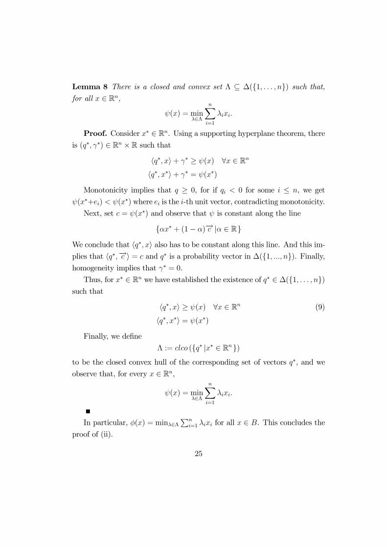
Lemma 8 There is a closed and convex set Λ ⊆ ∆({1, . . . , n}) such that,for all x ∈ Rn,
ψ(x) = minλ∈Λ
nXi=1
λixi.
Proof. Consider x∗ ∈ Rn. Using a supporting hyperplane theorem, there
is (q∗, γ∗) ∈ Rn ×R such that
hq∗, xi+ γ∗ ≥ ψ(x) ∀x ∈ Rn
hq∗, x∗i+ γ∗ = ψ(x∗)
Monotonicity implies that q ≥ 0, for if qi < 0 for some i ≤ n, we get
ψ(x∗+ei) < ψ(x∗) where ei is the i-th unit vector, contradicting monotonicity.
Next, set c = ψ(x∗) and observe that ψ is constant along the line
{αx∗ + (1− α)−→c |α ∈ R}
We conclude that hq∗, xi also has to be constant along this line. And this im-plies that hq∗,−→c i = c and q∗ is a probability vector in ∆({1, ..., n}). Finally,homogeneity implies that γ∗ = 0.
Thus, for x∗ ∈ Rn we have established the existence of q∗ ∈ ∆({1, . . . , n})such that
hq∗, xi ≥ ψ(x) ∀x ∈ Rn (9)
hq∗, x∗i = ψ(x∗)
Finally, we define
Λ := clco ({q∗ |x∗ ∈ Rn})
to be the closed convex hull of the corresponding set of vectors q∗, and we
observe that, for every x ∈ Rn,
ψ(x) = minλ∈Λ
nXi=1
λixi.
In particular, φ(x) = minλ∈ΛPn
i=1 λixi for all x ∈ B. This concludes the
proof of (ii).
25

5 References
Anscombe, F. J. and R. J. Aumann (1963), “A Definition of Subjective Prob-
ability”, The Annals of Mathematics and Statistics, 34: 199-205.
Bacharach, M. (1979), “Normal Bayesian Dialogues”, Journal of the Ameri-
can Statistical Association, 74: 837-846.
Bewley, T. (2002), “Knightian Decision Theory: Part I”, Decisions in Eco-
nomics and Finance, 25: 79-110. (Working paper, 1986).
Blackorby, C., D. Donaldson, and P. Mongin (2000), “Social Aggregation
Without the Expected Utility Hypothesis”, mimeo.
Bossert, W. (1997), “Uncertainty Aversion in Nonprobabilistic DecisionMod-
els,” Mathematical Social Sciences, 34: 191—203.
Bossert, W. and A. Slinko (2006), “Relative Uncertainty Aversion and Ad-
ditively Representable Set Rankings”, International Journal of Economic
Theory, 2: 105—122.
Chambers, C.P. and F. Echenique (2009), “When does aggregation reduce
uncertainty aversion”, mimeo.
Chambers, C.P. and T. Hayashi (2006), “Preference Aggregation under Un-
certainty: Savage vs. Pareto”, Games and Economic Behavior, 54: 430-440.
de Finetti, B. (1931), Sul Significato Soggettivo della Probabilità, Funda-
menta Mathematicae, 17: 298-329.
–––— (1937), “La Prevision: ses Lois Logiques, ses Sources Subjectives”,
Annales de l’Institut Henri Poincaré, 7: 1-68.
Ellsberg, D. (1961), “Risk, Ambiguity and the Savage Axioms”, Quarterly
Journal of Economics, 75: 643-669.
Fan, K. (1977), “Extension of invariant linear functionals”, Proceedings of
the American Mathematical Society, 66: 23—29.
26

Fishburn, P.C. (1970) Utility Theory for Decision Making. John Wiley and
Sons, 1970.
Gajdos, T., J.-M. Tallon, and J.-C. Vergnaud (2008), “Representation and
Aggregation of Preferences under Uncertainty”, Journal of Economic Theory,
141: 68—99.
Gajdos, T., T. Hayashi, J.-M. Tallon, and J.-C. Vergnaud (2008), “Attitude
toward imprecise information”, Journal of Economic Theory, 140: 27—65.
Gajdos, T., and J.-C. Vergnaud (2009), “Decisions with Conflicting and Im-
precise Information”, mimeo.
Genest, C., and J. Zidek (1986), “Combining Probability Distributions: A
Critique and an Annotated Bibliography”, Statistical Science, 1: 68—99.
Gilboa, I. (2009), Theory of Decision under Uncertainty, Econometric Society
Monograph Series, Cambridge University Press.
Gilboa, I., F. Maccheroni, M. Marinacci, and D. Schmeidler (2008), “Objec-
tive and Subjective Rationality in a Multiple Prior Model”, Econometrica,
forthcoming.
Gilboa, I., and M. Marinacci (2010), “Ambiguity and the Bayesian Ap-
proach”, mimeo.
Gilboa, I., A. Postlewaite, and D. Schmeidler (2008), “Probabilities in Eco-
nomic Modeling”, Journal of Economic Perspectives, 22: 173-188.
–––— (2009), “Is It Always Rational to Satisfy Savage’s Axioms?”, Eco-
nomics and Philosophy, forthcoming.
–––— (2010), “Rationality of Belief”, Synthese, forthcoming.
Gilboa, I., D. Samet, and D. Schmeidler (2004), “Utilitarian Aggregation of
Beliefs and Tastes”, Journal of Political Economy, 112: 932-938.
Gilboa, I. and D. Schmeidler (1989), “Maxmin Expected Utility with a Non-
Unique Prior”, Journal of Mathematical Economics, 18: 141-153.
27
Harsanyi, J. C. (1955), “Cardinal Welfare, Individualistic Ethics, and Inter-
personal Comparison of Utility”, Journal of Political Economy, 63: 309-321.
Hylland A. and R. Zeckhauser (1979), “The Impossibility of Bayesian Group
Decision Making with Separate Aggregation of Beliefs and Values”, Econo-
metrica, 6: 1321-1336.
Klibanoff, P., M. Marinacci, and S. Mukerji (2005), “A Smooth Model of
Decision Making under Ambiguity,” Econometrica, 73: 1849-1892.
Knight, F. H. (1921), Risk, Uncertainty, and Profit. Boston, New York:
Houghton Mifflin.
List, C. and P. Pettit (2002), “Aggregating Sets of Judgments: An Impossi-
bility Result”, Economics and Philosophy, 18: 89-110.
McConway, K. J. (1981), “Marginalization and Linear Opinion Pools”, Jour-
nal of the American Statistical Association, 76: 410-414.
Mongin, P. (1995), “Consistent Bayesian Aggregation”, Journal of Economic
Theory, 66: 313-351.
Nau, R.F. (2006), “Uncertainty Aversion with Second-Order Utilities and
Probabilities”, Management Science 52: 136-145.
Ramsey, F. P. (1931), “Truth and Probability”, in The Foundation of Math-
ematics and Other Logical Essays. New York: Harcourt, Brace and Co.
Savage, L. J. (1954), The Foundations of Statistics. New York: John Wiley
and Sons. (Second addition in 1972, Dover)
Schaefer, H. H. (1971), Topological Vector Spaces. New York: Springer Verlag
(3rd printing).
Schmeidler, D. (1986), “Integral Representation without Additivity”, Pro-
ceedings of the American Mathematical Society, 97: 255-261.
–––— (1989), “Subjective Probability and Expected Utility without Ad-
ditivity”, Econometrica, 57: 571-587.
28

Seo, K. (2009), “Ambiguity and Second-Order Belief”, Econometrica, 67:1575-1605.
Stone, M. (1961), “The Linear Opinion Pool”, Annals of Mathematical Sta-
tistics, 32: 1339-1342.
von Neumann, J. and O. Morgenstern (1944), Theory of Games and Eco-
nomic Behavior. Princeton, N.J.: Princeton University Press.
Stephane Zuber (2009), “Harsanyi’s Theorem without the Sure-Thing Prin-
ciple”, mimeo.
29

6 Appendix for Referees
6.1 Proof of Lemma 6
We define ψ by ψ(x) := supP
k αkφ(xk), where the supremum is taken over
all finite families xk ∈ cone(B), αk ≥ 0, (k = 1, . . . ,K), such thatP
k αk = 1
and x ≥P
k αkxk.
Homogeneity: Let there be given x and β > 0. Since β may be larger or
smaller than 1, it suffices to show that
ψ(βx) ≥ βψ(x).
Let there be given xk ∈ cone(B), αk ≥ 0, (k = 1, . . . ,K), such thatP
k αk =
1 and x ≥P
k αkxk. Define x0k = βxk ∈ cone(B). Then
βx ≥Xk
αkβxk =Xk
αkx0k
and it follows that
ψ(βx) ≥Xk
αkφ(x0k) =
Xk
αkφ(βxk) = βXk
αkφ(xk)
As this holds for any pair of sequences {xk} , {αk}, and ψ(x) is the supremumover the respective
Pk αkφ(xk), the conclusion follows.
Shift : Let there be given x and c ∈ R. Since cmay be positive or negative,it suffices to show that
ψ(x+−→c ) ≥ ψ(x) + c.
Consider xk ∈ cone(B), αk ≥ 0, (k = 1, . . . ,K), such thatP
k αk = 1 and
x ≥P
k αkxk. Define x0k = xk +−→c ∈ cone(B). Observe that
x+−→c ≥Xk
αkx0k =
Xk
αk(xk +−→c )
hence
ψ(x+−→c ) ≥Xk
αkφ(xk + c) =Xk
αkφ(xk) + c.
As this holds for any pair of sequences {xk} , {αk}, and ψ(x) is the supremumover the respective
Pk αkφ(xk), the conclusion follows.
30

6.2 Details of proof of Lemma 7
We show that ψ satisfies monotonicity, concavity, homogeneity and Shift:
Monotonicity: Consider y, z ∈ Rn such that y ≥ z. Then any x ∈ D such
that x ≤ z also satisfies x ≤ y and it follows that ψ(y) ≥ ψ(z).
Concavity: Let y, z ∈ Rn and α ∈ [0, 1]. We wish to show that
ψ(αy + (1− α)z) ≥ αψ(y) + (1− α)ψ(z).
For ε > 0, let xy, xz ∈ D be such that y ≥ xy, z ≥ xz and
ψ(y) < ψ(xy) + ε
ψ(z) < ψ(xz) + ε
This means that
αψ(y) + (1− α)ψ(z) < αψ(xy) + (1− α)ψ(xz) + ε
Since D is convex, αxy + (1− α)xz ∈ D. Because ψ is concave on D,
ψ(αxy + (1− α)xz) ≥ αψ(xy) + (1− α)ψ(xz)
and thus
ψ(αxy + (1− α)xz) > αψ(y) + (1− α)ψ(z)− ε.
Next, observe that y ≥ xy, z ≥ xz imply
αy ≥ αxy
(1− α)z ≥ (1− α)xz
and
αy + (1− α)z ≥ αxy + (1− α)xz
By definition of ψ,
ψ(αy + (1− α)z) ≥ ψ(αxy + (1− α)xz)
31

and thus
ψ(αy + (1− α)z) > αψ(y) + (1− α)ψ(z)− ε
for all ε > 0, which means that ψ is concave.
Homogeneity: Consider y ∈ Rn and α > 0. We wish to show that
ψ(αy) = αψ(y)
It suffices to show
ψ(αy) ≥ αψ(y)
(because α can be larger or smaller than 1.) Consider, then, ε > 0 and
xy ∈ D such that y ≥ xy and
ψ(y) < ψ(xy) + ε.
Since ψ is homogenous on D,
ψ(αxy) = αψ(xy)
Moreover,
αy ≥ αxy
and thus
ψ(αy) ≥ ψ(αxy) = αψ(xy) > αψ(y)− αε
This being true for all ε > 0, we conclude that ψ(αy) ≥ αψ(y).
Shift : Let there be given y ∈ Rn and c ∈ R. We wish to show that
ψ(y +−→c ) = ψ(y) + c.
It suffices to show that (for all y ∈ Rn and c ∈ R)
ψ(y +−→c ) ≥ ψ(y) + c
observe that, for every x ∈ D such that x ≤ y, we have x + −→c ∈ D and
x+−→c ≤ y +−→c . Thus,
ψ(y +−→c ) ≥ ψ(x+−→c ) = ψ(x) + c
32

where the last equality follows from the fact that ψ satisfies Shift on D.
Taking the supremum on the right hand side, we obtain the conclusion that
ψ(y +−→c ) ≥ ψ(y) + c.
33