12.10.2012 - catherine wolfram
DESCRIPTION
How Pro-Poor Growth will Affect the Global Demand for EnergyTRANSCRIPT
How Pro-Poor Growth Will Affect the Global Demand for Energy
Alan Fuchs Paul Gertler Orie Shelef
and Catherine Wolfram
UC Berkeley
December 2012

Wolfram 1

Wolfram 2

Wolfram 3

The developing world accounts for most expected growth in energy and CO2 emissions.
Wolfram 4
Source: Energy Information Administration.

Pro-poor growth
• Many countries have made progress addressing poverty recently.
• China, for instance, saw the share of it’s population living in poverty fall from 53% in 1981 to 8% in 2001.
• Brazil and Mexico have aggressive anti-poverty programs.
• The success fighting poverty varies around the world.
Wolfram 5
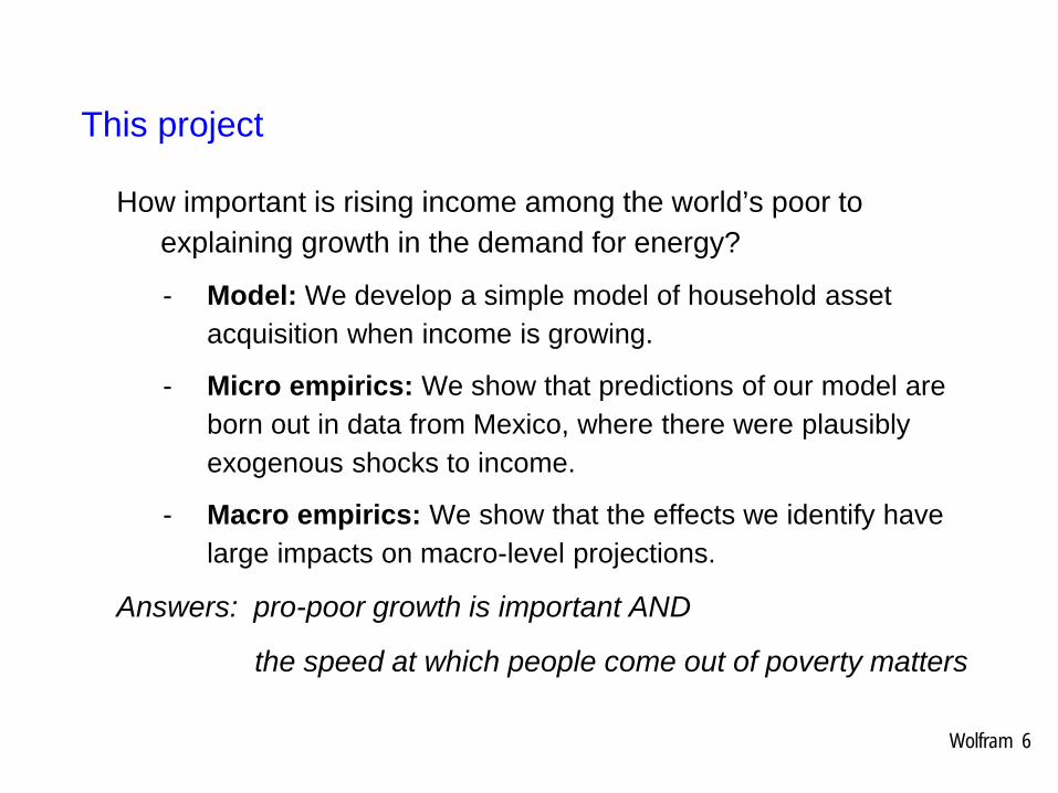
This project
How important is rising income among the world’s poor to explaining growth in the demand for energy?
- Model: We develop a simple model of household asset acquisition when income is growing.
- Micro empirics: We show that predictions of our model are born out in data from Mexico, where there were plausibly exogenous shocks to income.
- Macro empirics: We show that the effects we identify have large impacts on macro-level projections.
Answers: pro-poor growth is important AND
the speed at which people come out of poverty matters
Wolfram 6

Wolfram 7
Wolfram 8
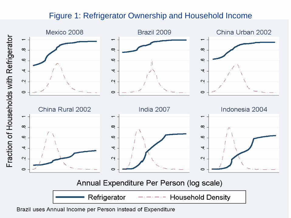
Figure 1: Refrigerator Ownership and Household Income

Benchmarking EIA’s projections
Wolfram 9
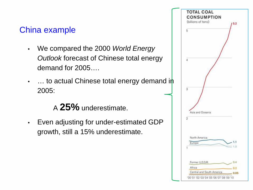
China example
• We compared the 2000 World Energy Outlook forecast of Chinese total energy demand for 2005….
• … to actual Chinese total energy demand in 2005:
A 25% underestimate.
• Even adjusting for under-estimated GDP growth, still a 15% underestimate.

Why it’s important to project energy demand
• Fossil fuel use is the major contributor to climate change. - Emissions projections inform likely damages.
- Country-by-country emissions projections are used to establish baselines for global negotiations.
• Infrastructure investment require long lead times. - Incorrect demand forecasts can lead to local shortages and
global price spikes.
Wolfram 11

Outline
• Model describes tradeoff between lumpy asset (refrigerator) and continuous consumption (food).
• Empirical evidence from Mexico.
- Acquisition of refrigerators and other assets.
- Energy use conditional on asset holdings.
• Cross-country estimates of energy “income elasticities,” which are typical inputs to forecast models.
Wolfram 12

Model setup
• Two periods, no discounting.
• Each period, household consumes at most two goods:
- Consumption good (food) with utility uf(.), uf’(.)>0, uf’’(.)<0.
- Durable good (refrigerator) fixed per-period utility R. – Later we’ll let R vary by household.
• Per period income Y.
• Household cannot borrow (credit constraints),
• … but can save S ∈{0,Y}.
Wolfram 13

Model setup II
• Price of food normalized to 1.
• Price of refrigerator = P.
• Y < P (refrigerator too expensive to purchase in first period).
• Household chooses consumption of two goods to maximize two-period utility.
• No complementarities between goods
- i.e., in our model, you don’t put food in the refrigerator…
Wolfram 14
Our underlying assumptions are consistent with the development literature.
• Declining marginal utility of food.
- Engel (1895) showed that the fraction of consumption devoted to food declines with consumption.
• Credit constraints.
- Banerjee, Duflo, Glennerster and Kinnan (2010).
• Refrigerators expensive.
Wolfram 15

Model graphically
Income (Y)
Mar
gina
l Util
ity
Y
u’f (Y)
Area = per-period utility of refrigerator (R/2)
2PY−
PR
2P
Wolfram 16 Note: the graph is drawn for a single period, and the model has two identical periods.

Relationship between income and durable purchase
Income (Y)
Mar
gina
l Util
ity
Y
u’f (Y)
2PY−
PRH High R buys refrigerator.
• Saves P/2 in period 1. • Spends P/2 + S in period 2.
Wolfram 17

Relationship between income and durable purchase
Income (Y)
Mar
gina
l Util
ity
Y
u’f (Y)
2PY−
PRL
Low R doesn’t buy refrigerator.
Wolfram 18

Relationship between income and durable purchase
Income (Y)
Mar
gina
l Util
ity
Y
u’f (Y)
2PY−
PRM
Medium R just indifferent. Red area (lost utility from consuming fridge) = Green area (gained utility)
Wolfram 19
Refrigerator ownership as a function of income.
Our first empirical prediction:
Given unrestrictive assumptions on distribution of Y and R in the population, this model predicts an S-shaped relationship between income and durable ownership.
- Micro foundation for Bonus (1973), who modeled durable acquisition.
- Many development economists have noted S-shaped relationship without an underlying model.
– Dargay, Dermot and Sommer, 2007
– Koptis and Cropper, 2005
Wolfram 20

Refrigerator ownership as a function of changes in income.
• Does the pace at which Y changes affect refrigerator acquisition as a function of income?
- We will relate changes in Y to growth shortly.
• Consider the case where a household receives transfers.
- 2T over two periods.
- We’ll compare:
– Even case (T1 = T2 = T)
– Uneven case (T1 < T2; T1 + T2 = 2T)
– Both cases have same cumulative transfers (2T)
Wolfram 21

RL in even transfer case (no refrigerator purchase)
Income (Y)
Mar
gina
l Util
ity
Y + T
u’f (Y)
2PTY −+
PRL
Wolfram 22

Same RL will purchase a refrigerator in the uneven transfer case
Income (Y)
Mar
gina
l Util
ity
Y + T
u’f (Y)
1TY +
PRL
Assume T – T1 = (For now, to make the picture simpler.)
2P
Y + T2
2P
2P
Wolfram 23

Same conclusion, though slightly more complicated graph, with a smaller difference between T1 and T2
Income (Y)
Mar
gina
l Util
ity
Y + T
u’f (Y)
New1TY +
PRL2
S = savings
S
New2TY +
Lost utility from saving in period 1
Wolfram 24
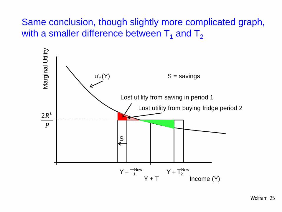
Same conclusion, though slightly more complicated graph, with a smaller difference between T1 and T2
Income (Y)
Mar
gina
l Util
ity
Y + T
u’f (Y)
New1TY +
PRL2
S = savings
S
New2TY +
Lost utility from saving in period 1
Lost utility from buying fridge period 2
Wolfram 25
Refrigerator ownership as a function of changes in income
Second empirical prediction:
Holding total transfers constant, delaying some transfers from the first period to the second period increases asset acquisition.
- “Forced savings” effect.
- “Complementary savings” effect.
Wolfram 26
Interaction between delay and level of transfers
Third empirical prediction:
We also show that the effect of increasing transfers [2T*(1 + α)] on durable acquisition is smaller for households receiving equal transfers between periods 1 and 2.
Wolfram 27

Our result suggest that current income is not the only determinant of asset ownership. The path matters, too.
•Fast growth countries will have higher refrigerator penetration over time. •Both because they’re richer, and because of our complementary savings effect.
Wolfram 28

Outline
• Model describes tradeoff between lumpy asset (refrigerator) and continuous consumption (food).
• Empirical evidence from Mexico.
- Acquisition of refrigerators and other assets.
- Energy use conditional on asset holdings.
• Cross-country estimates of energy “income elasticities,” which are typical inputs to forecast models.
Wolfram 29
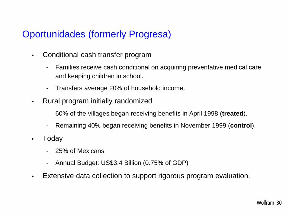
Oportunidades (formerly Progresa)
• Conditional cash transfer program
- Families receive cash conditional on acquiring preventative medical care and keeping children in school.
- Transfers average 20% of household income.
• Rural program initially randomized
- 60% of the villages began receiving benefits in April 1998 (treated).
- Remaining 40% began receiving benefits in November 1999 (control).
• Today
- 25% of Mexicans
- Annual Budget: US$3.4 Billion (0.75% of GDP)
• Extensive data collection to support rigorous program evaluation.
Wolfram 30

Growth in appliance ownership over time by consumption level
31 Source: Mexico Encuesta Nacional de Ingreso y Gasto de los Hogares (1996, 1998, 2000, 2002, 2004, 2006, 2008). See data appendix for details.
Figure 4: Growth in Refrigerator Ownership by Consumption Quartile for Mexico
0%
10%
20%
30%
40%
50%
60%
70%
80%
90%
100%
1994 1996 1998 2000 2002 2004 2005 2006 2008
Shar
e of
Hou
seho
lds w
ith R
efrig
erat
or
1st Decile 2nd Decile 3rd Decile 4th-10th Deciles
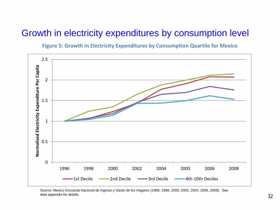
Growth in electricity expenditures by consumption level
32
Figure 5: Growth in Electricity Expenditures by Consumption Quartile for Mexico
0
0.5
1
1.5
2
2.5
1996 1998 2000 2002 2004 2005 2006 2008
Nor
mal
ized
Ele
ctric
ity E
xpen
ditu
re P
er C
apita
1st Decile 2nd Decile 3rd Decile 4th-10th Deciles
Source: Mexico Encuesta Nacional de Ingreso y Gasto de los Hogares (1996, 1998, 2000, 2002, 2004, 2006, 2008). See data appendix for details.

Empirical predictions – nonlinear wealth effect
Household that were richer at baseline will be: • More likely to
purchase a refrigerator at any cumulative transfer level, and
• More responsive to increases in cumulative transfers.
Wolfram 33
Richer
Poorer

Graphical evidence for relative wealth
34
Wolfram 35
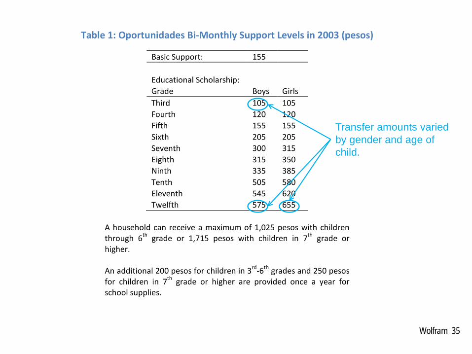
Table 1: Oportunidades Bi-Monthly Support Levels in 2003 (pesos)
A household can receive a maximum of 1,025 pesos with children through 6th grade or 1,715 pesos with children in 7th grade or higher. An additional 200 pesos for children in 3rd-6th grades and 250 pesos for children in 7th grade or higher are provided once a year for school supplies.
Basic Support: 155 Educational Scholarship: Grade Boys Girls Third 105 105 Fourth 120 120 Fifth 155 155 Sixth 205 205 Seventh 300 315 Eighth 315 350 Ninth 335 385 Tenth 505 580 Eleventh 545 620 Twelfth 575 655
Transfer amounts varied by gender and age of child.
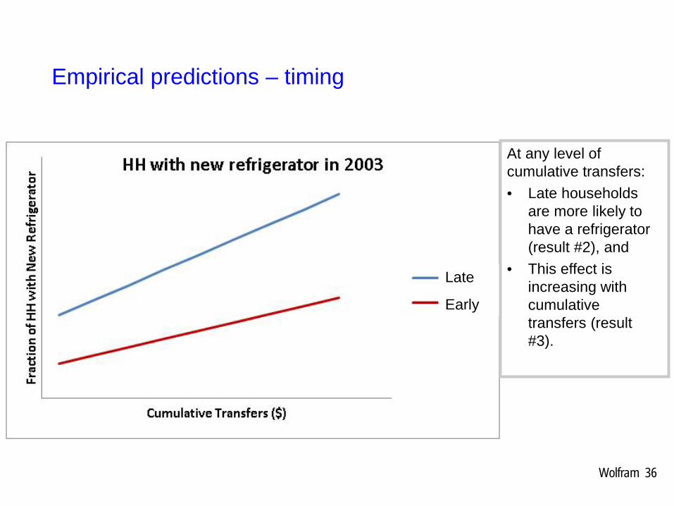
Empirical predictions – timing
Wolfram 36
Late
Early
At any level of cumulative transfers: • Late households
are more likely to have a refrigerator (result #2), and
• This effect is increasing with cumulative transfers (result #3).

How much overlap is there between early and late households in cumulative transfer amounts?
37

Graphical evidence on timing effects
Wolfram 38
Discrete-time hazard specification – result 1
Wolfram 39
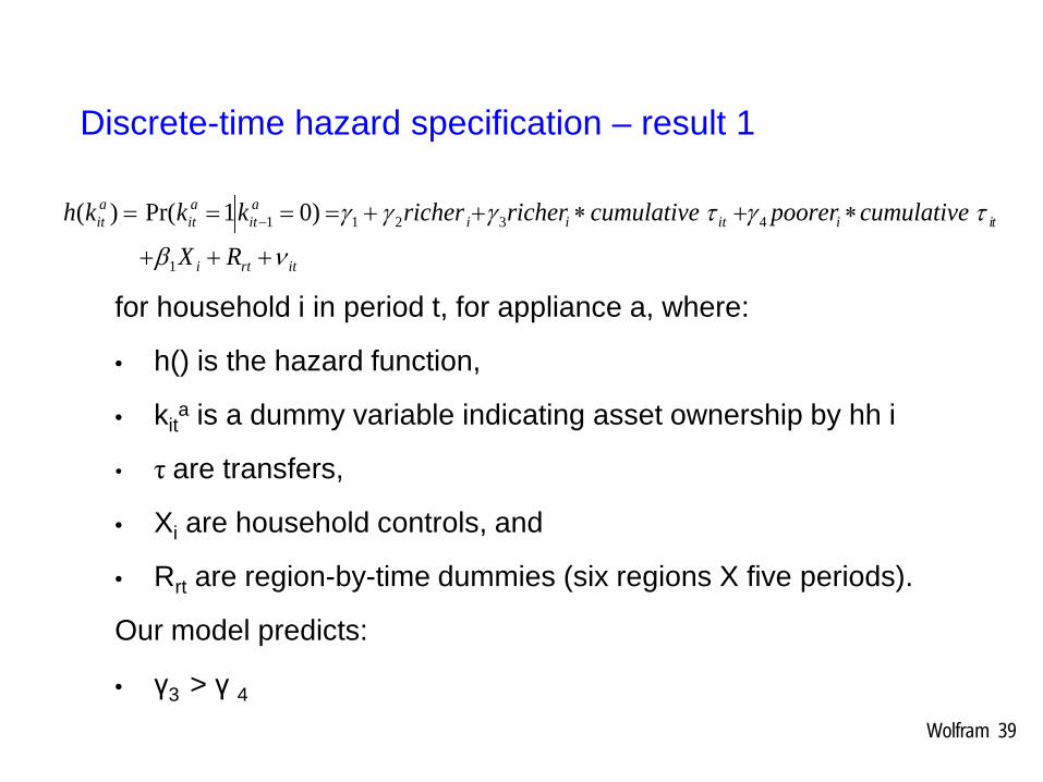
for household i in period t, for appliance a, where:
• h() is the hazard function,
• kita is a dummy variable indicating asset ownership by hh i
• τ are transfers,
• Xi are household controls, and
• Rrt are region-by-time dummies (six regions X five periods).
Our model predicts:
• γ3 > γ 4
itrti
tiiitiiait
ait
ait
RX
cumulativepoorercumulativericherricherkkkh
νβ
τγτγγγ
+++
∗+∗++==== −
1
43211 )01Pr()(

Discrete-time hazard specification – results 2 & 3
Wolfram 40
Our model predicts:
• α2 > 0 ; α3 ,α4 < 0
itrti
tiiiitait
ait
ait
RX
cumulativeearlyearlycumulativekkkh
νβ
τααταα
+++
∗+++==== −
1
43211 )01Pr()(

Table 4: Basic Results - Refrigerator - Income Effects
(1) (2) (3) (4) (5) (6)
OLS IV IV OLS IV IV Discrete Time Hazard Household FE Discrete Time Hazard Household FE Cumulative Transfers 0.023*** 0.029*** 0.048*** [0.004] [0.005] [0.005] Cumulative Transfers X Bottom 75% of Baseline Assets
0.020*** 0.024*** 0.043*** [0.004] [0.005] [0.005]
Cumulative Transfers X Top 25% of Baseline Assets
0.032*** 0.040*** 0.058*** [0.006] [0.007] [0.007]
N 30,414 30,414 30,258 30,414 30,414 30,258 R-squared 0.100 0.100
F Stat on Excluded Variables - Cumulative Transfers
3156 2262
F Stat on Excluded Variables - Cumulative Transfers X Bottom 75% 3161 3767 F Stat on Excluded Variables - Cumulative Transfers X Top 25% 1635 1596 Number of Households 6,655 6,655
Results for refrigerators – prediction 1
Wolfram 41
Relatively better off are more sensitive, consistent w/ prediction 1.
Note: All specifications include state by round- fixed effects and household controls. Robust standard errors clustered by village in brackets.

Table 5: Basic Results – Refrigerator - Timing
(1) (2) (3) (4) (5)
OLS OLS OLS IV IV
Discrete Time Hazard Household FE Cumulative Transfers
0.023*** 0.028*** 0.039*** 0.056*** 0.061*** [0.004] [0.004] [0.007] [0.007] [0.007]
Early
-0.016*** -0.007 -0.009* [0.005] [0.005] [0.005]
Cumulative Transfers X Early
-0.015** -0.021*** -0.018** [0.006] [0.007] [0.007]
Net Early Effect at 2003 Median Cumulative Transfers
-0.025*** -0.033*** [0.008] [0.008]
N 30,414 30,414 30,414 30,414 30,258 R-squared 0.100 0.100 0.101 F Stat on Excluded Variables - Cumulative Transfers 1,554 1,226 F Stat on Excluded Variables - Cumulative Transfers X Status 1,974 1,889 Number of Households 6,655
Results for refrigerators – predictions 2&3
Wolfram 42 Note: All specifications include state by round- fixed effects and household controls. Robust standard errors clustered by village in brackets.
Consistent w/ prediction 2.
Consistent w/ prediction 3.

Additional results
• Patterns seems to hold with other durables.
• “Placebo” tests: cumulative transfer amounts do not consistently predict asset ownership at baseline.
• If anything future income is negatively correlated with asset acquisition, consistent with a “complementary savings” explanation.
• Using these results as a first-stage, we see that asset ownership is the only way in which increased transfers drive energy use.
- i.e., there’s no effect of transfers on electricity use once you condition on appliance ownership.
Wolfram 43

The developing world accounts for most forecast growth in energy use.
Wolfram 44
What would our model suggest about EIA’s forecasts?
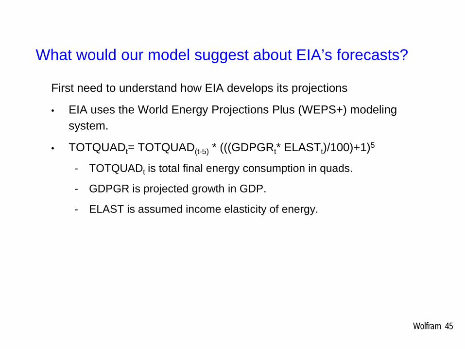
First need to understand how EIA develops its projections
• EIA uses the World Energy Projections Plus (WEPS+) modeling system.
• TOTQUADt= TOTQUAD(t-5) * (((GDPGRt* ELASTt)/100)+1)5
- TOTQUADt is total final energy consumption in quads.
- GDPGR is projected growth in GDP.
- ELAST is assumed income elasticity of energy.
Wolfram 45
Does EIA’s methodology allow for differences between countries with pro-poor growth?
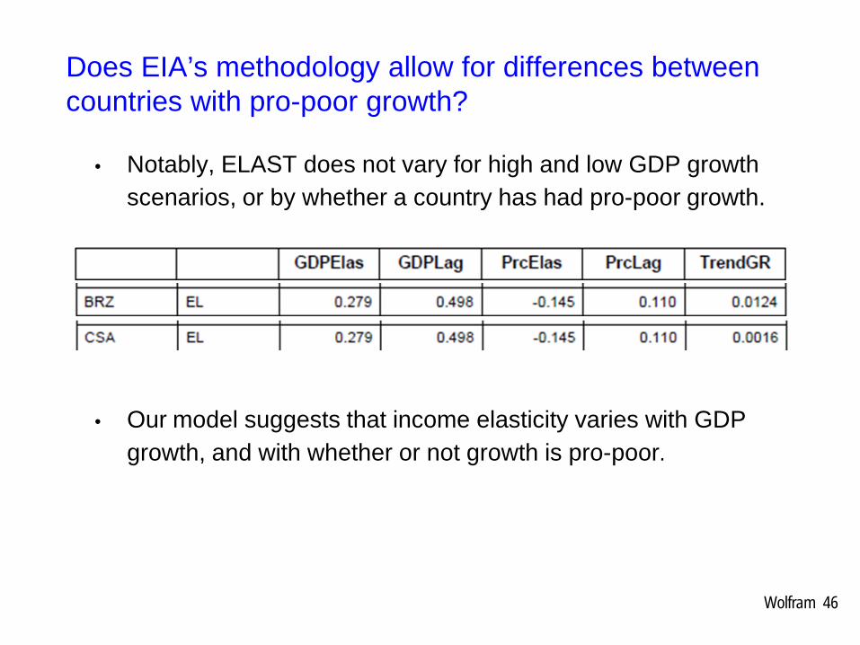
• Notably, ELAST does not vary for high and low GDP growth scenarios, or by whether a country has had pro-poor growth.
• Our model suggests that income elasticity varies with GDP growth, and with whether or not growth is pro-poor.
Wolfram 46
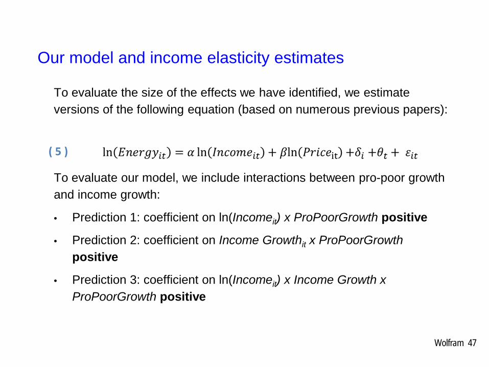
Our model and income elasticity estimates
To evaluate the size of the effects we have identified, we estimate versions of the following equation (based on numerous previous papers):
To evaluate our model, we include interactions between pro-poor growth and income growth:
• Prediction 1: coefficient on ln(Incomeit) x ProPoorGrowth positive
• Prediction 2: coefficient on Income Growthit x ProPoorGrowth positive
• Prediction 3: coefficient on ln(Incomeit) x Income Growth x ProPoorGrowth positive
Wolfram 47
( 5 )

Cross-country income elasticity estimates
Wolfram 48
T a b le 9 : A gg re g at e C o u nt ry -L e ve l E n e rg y C on su m p tio n
(1 ) (2 ) (3 )
V A R IA B L E S
ln ( In c o m e ) 0 .9 2 5 * * * 0 .8 5 6 * * * 0 .9 0 9 ** *
[0 .0 8 7 ] [0 . 1 0 4 ] [0 .0 8 8 ]
In c o m e G ro w th
-0 .3 2 4 0 .3 0 7
[0 . 2 0 1 ] [0 .7 2 6 ]
ln ( In c o m e ) X In co m e G ro w t h
0 .0 9 7
[0 .1 1 6 ]
ln ( In c o m e ) X P ro P o o rG ro w th 0 .0 7 3 * * *
0 .0 5 7 ** *
[0 .0 1 7 ]
[0 .0 1 6 ]
In c o m e G ro w th X P ro P o o rG ro w th
0 .1 2 2 * * 0 .8 9 3 ** *
[0 . 0 5 3 ] [0 .2 3 3 ]
In c o m e X I n c o m e G ro w th X P ro P o o rG ro w th
0 .1 4 6 ** *
[0 .0 3 7 ]
C o u n try F ix e d E f fe c ts Y E S Y E S Y E S
Y e a r F ix e d E ffe c ts Y E S Y E S Y E S
O b s e rva tio n s 9 0 7 8 9 2 8 9 2 R -sq u a re d 0 .9 8 1 0 . 9 8 1 0 .9 8 3 R o b u s t s ta n d a rd e r ro rs c l u s te re d b y co u n t ry i n b ra ck e ts . * * * p < 0 .0 1 , * * p < 0 .0 5 , * p < 0 .1 0 .
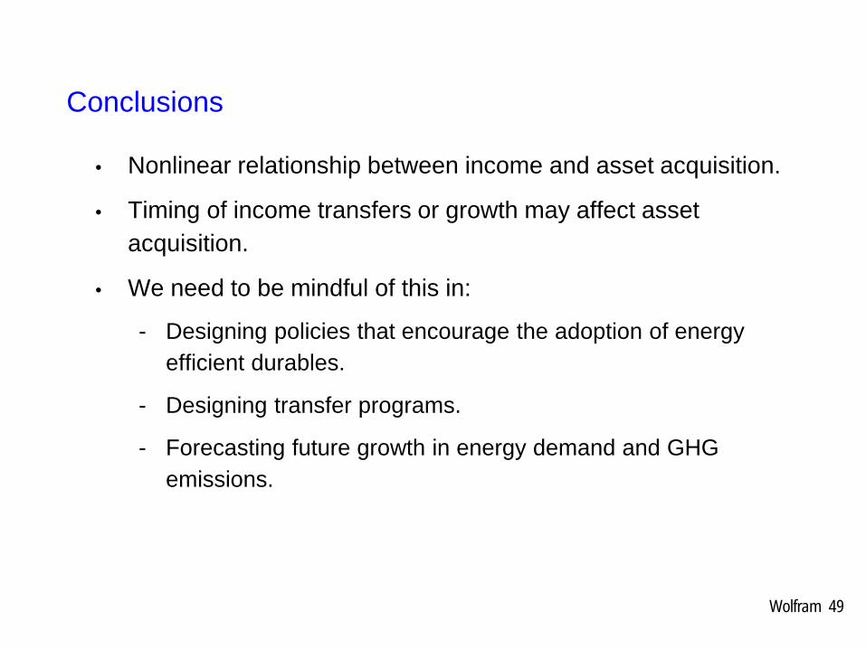
Conclusions
• Nonlinear relationship between income and asset acquisition.
• Timing of income transfers or growth may affect asset acquisition.
• We need to be mindful of this in:
- Designing policies that encourage the adoption of energy efficient durables.
- Designing transfer programs.
- Forecasting future growth in energy demand and GHG emissions.
Wolfram 49

Wolfram 50