ChE 310 Problem Set 12 Due Friday 12/13/19

Note: this assignment will be ungraded, so no submission is required. However, there is one optional extra credit problem available. For this problems, collect all m-files in a single .zip file and upload the .zip file to the course webpage by midnight on Friday, December 13, 2019. Please note any collaborations in comments. Each student must upload their own unique copy of the work.

12_1. Solve Chapra problem 23.13. How many data points are generated by MATLAB when using ode45 vs. ode23s?

NOTE: There is a typo in the third differential equation in the book (has one extra (-) sign):

d c3

dt=0.013 c1−1000 c1c3−2500 c2c3

Solution:

%ps12_1%Coded by LTR on 12/5/19%Chapra problem 23.13 clear; clf; %First create subfunction below %Solve with ode45 subplot(1,2,1)[t, C] = ode45(@ps12_1_func,[0 50],[1 1 0]);c1 = C(:,1); c2 = C(:,2); c3 = C(:,3);

plot(t,c1,'ko-'); hold on;plot(t,c2,'rd-');plot(t,c3,'bs-');xlabel('t')ylabel('c')title('ode45')legend('c1','c2','c3')num_terms_ode45 = length(t) %Solve w/ode23ssubplot(1,2,2)[t, C] = ode23s(@ps12_1_func,[0 50],[1 1 0]);c1 = C(:,1); c2 = C(:,2); c3 = C(:,3);plot(t,c1,'ko-'); hold on;plot(t,c2,'rd-');plot(t,c3,'bs-');xlabel('t')ylabel('c')title('ode23s')legend('c1','c2','c3')num_terms_ode23s = length(t) function dCdt = ps12_1_func(t,C)c1 = C(1); c2 = C(2); c3 = C(3);dc1dt = -0.013*c1-1000*c1.*c3;dc2dt = -2500*c2.*c3;dc3dt = 0.013*c1-1000*c1.*c3-2500*c2.*c3;dCdt = [dc1dt; dc2dt; dc3dt];end

Output:

num_terms_ode45 =

163881

num_terms_ode23s =

18

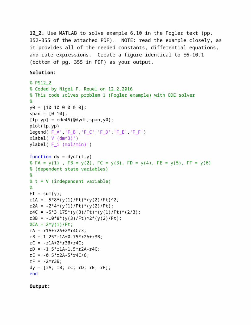
12_2. Use MATLAB to solve example 6.10 in the Fogler text (pp. 352-355 of the attached PDF). NOTE: read the example closely, as it provides all of the needed constants, differential equations, and rate expressions. Create a figure identical to E6-10.1 (bottom of pg. 355 in PDF) as your output.

Solution:

% PS12_2% Coded by Nigel F. Reuel on 12.2.2016% This code solves problem 1 (Fogler example) with ODE solver%y0 = [10 10 0 0 0 0];span = [0 10];[tp yp] = ode45(@dydt,span,y0);plot(tp,yp)legend('F_A','F_B','F_C','F_D','F_E','F_F')xlabel('V (dm^3)')ylabel('F_i (mol/min)') function dy = dydt(t,y)% FA = y(1) , FB = y(2), FC = y(3), FD = y(4), FE = y(5), FF = y(6)% (dependent state variables)%% t = V (independent variable)%Ft = sum(y);r1A = -5*8*(y(1)/Ft)*(y(2)/Ft)^2;r2A = -2*4*(y(1)/Ft)*(y(2)/Ft);r4C = -5*3.175*(y(3)/Ft)*(y(1)/Ft)^(2/3);r3B = -10*8*(y(3)/Ft)^2*(y(2)/Ft);%CA = 2*y(1)/Ft;rA = r1A+r2A+2*r4C/3;rB = 1.25*r1A+0.75*r2A+r3B;rC = -r1A+2*r3B+r4C;rD = -1.5*r1A-1.5*r2A-r4C;rE = -0.5*r2A-5*r4C/6;rF = -2*r3B;dy = [rA; rB; rC; rD; rE; rF];end Output:

12_3

Consider the following system of differential equations resulting from a series of reactions:

dC A

dt=−k1C A−k2C ACB

dCB

dt=2k1CA−k2C ACB−k3CBCC

dCC

dt=2k2C ACB−k3CBCC

dCD

dt=k3CBCC−k4CD

(A)We know the initial conditions C A0=20 molL , and CB0=CC 0=C D0=0. We precisely

measure the concentrations after one minute: C A=3.25 molL ; CB=0.25 mol

L ;

CC=8 molL

;CD=7.5 molL . Use this information to solve for the actual values of

k1 , k2 , k3 , k4. (Assume your measurements after one minute are perfect.)(B) Component D is a product of interest. At what time should we stop the reaction to

maximize the concentration of component D? Use the results of part (A), and be precise.

Solution:

%PS12_3%Coded by LTR on 12/5/19 %If interested, the reactions considered are:%A --> 2B%A + B --> 2C%B + C --> D%D --> E clear; clf; %First create a subfunction with the differential equations.%This is ps12_3_odefunc %Part A%Create a second subfunction that's set up to do the fsolve.%This is ps12_3_fsolveCobs = [3.25 0.25 8 7.5];k = fsolve(@ps12_3_fsolve,[1 2 3 .5],[],@ps12_3_odefunc,Cobs);k1 = k(1), k2 = k(2), k3 = k(3), k4 = k(4)

%plot with the final values of k[t,C] = ode45(@ps12_3_odefunc,[0 5],[20 0 0 0],[],k);plot(t,C)legend('CA','CB','CC','CD') %part B%Create a third subfunction ps12_3_max%Solve with fminsearch, pass best values of k[t_maxD, v_maxD_neg]=fminsearch(@ps12_3_max,2,[],@ps12_3_odefunc,k);t_maxDv_maxD = -v_maxD_neg function dCdt = ps12_3_odefunc(t,C,k)%There are a few ways to do this, but for now we'll treat k as a passed%parameter vector with the 4 individual k values.%Unpack our variables to a more usable form:CA = C(1); CB = C(2); CC = C(3); CD = C(4);k1 = k(1); k2 = k(2); k3 = k(3); k4 = k(4); %Write differential equationsdCAdt = -k1*CA - k2*CA*CB;dCBdt = 2*k1*CA-k2*CA*CB-k3*CB*CC;dCCdt = 2*k2*CA*CB-k3*CB*CC;dCDdt = k3*CB*CC-k4*CD; %RepackagedCdt = [dCAdt; dCBdt; dCCdt; dCDdt];end function C_diff = ps12_3_fsolve(k,odefun,C_obs)%Subfunction that manipulates k values to fit the given ODE to match the%observed C values.[t, C] = ode45(odefun,[0 1],[20 0 0 0],[],k);CA = C(end,1); CB = C(end,2); CC = C(end,3); CD = C(end,4);%Create "root-finding functions"CA_diff = CA - C_obs(1); CB_diff = CB - C_obs(2); CC_diff = CC - C_obs(3); CD_diff = CD - C_obs(4);%Package our differences to one output for fsolve to work withC_diff = [CA_diff; CB_diff; CC_diff; CD_diff];end function CD_out = ps12_3_max(t_end,odefun,k)%Solve ODE to time t_end[t, C] = ode45(odefun,[0 t_end],[20 0 0 0],[],k);%output value of CD at t_end; negative for maximizingCD_out = -C(end,4);end

Output:

k1 =

1.0004

k2 =

1.7602

k3 =

2.6463

k4 =

0.2383

t_maxD =

1.8227

v_maxD =

8.6730

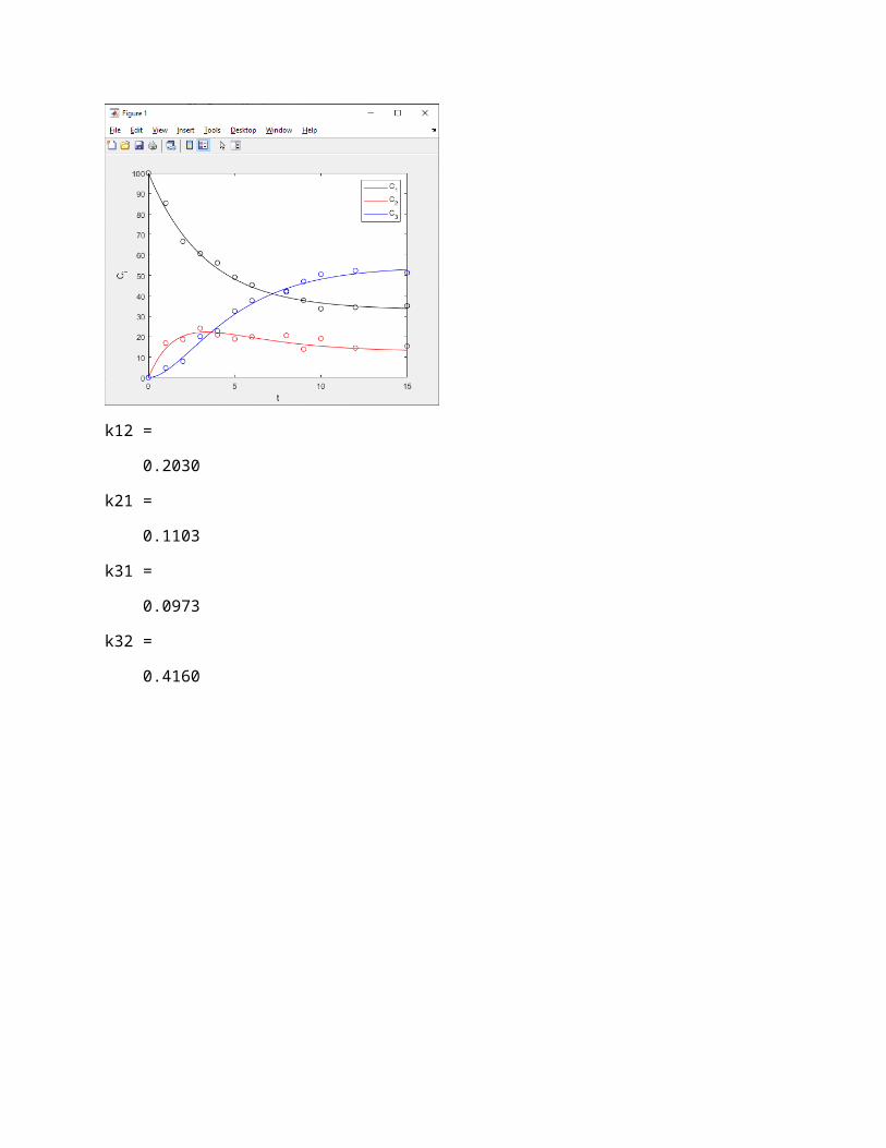
12_4. Solve problem 23.32 in the 4th edition of the Chapra text.

Solution:

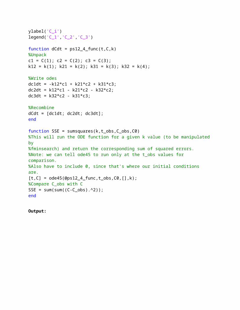
%PS12_4.m%Solves problem 23.32 in Chapra 4th ed%Coded by LTR on 12/5/19 clear; clf; C0 = [100 0 0]; %Data import. Note that we're also adding the values at t = 0,%since that makes things easier for running the ODE solver + comparison%later on. Transposing these to match the shape of ODE solution outputs. t_obs = [0:6 8:10 12 15]'; %times from data tableC_obs = [100 85.3 66.6 60.6 56.1 49.1 45.3 41.9 37.8 33.7 34.4 35.1; 0 16.9 18.7 24.1 20.9 18.9 19.9 20.6 13.9 19.1 14.5 15.4; 0 4.7 7.9 20.1 22.8 32.5 37.7 42.4 47 50.5 52.3 51.3]'; %First, make subfunction containing ODEs (ps12_4_func).%k is a passed parameter. %Next, make an optimization subfunction. This will run ps12_4_func for given%k, and calculate the sum of squared error compared with C_obs. %Last, call the optimization function with the recommended initial guess.[k, SSE] = fminsearch(@sumsquares,[0.15 0.15 0.15 0.15],[],t_obs,C_obs,C0);k12 = k(1), k21 = k(2), k31 = k(3), k32 = k(4) %Plot results, for comparison and checking work.[t,C] = ode45(@ps12_4_func,[0 15],C0,[],k);plot(t,C(:,1),'k-'), hold onplot(t,C(:,2),'r-')plot(t,C(:,3),'b-')plot(t_obs,C_obs(:,1),'ko')plot(t_obs,C_obs(:,2),'ro')plot(t_obs,C_obs(:,3),'bo')xlabel('t')ylabel('C_i')legend('C_1','C_2','C_3') function dCdt = ps12_4_func(t,C,k)%Unpackc1 = C(1); c2 = C(2); c3 = C(3);k12 = k(1); k21 = k(2); k31 = k(3); k32 = k(4); %Write odes

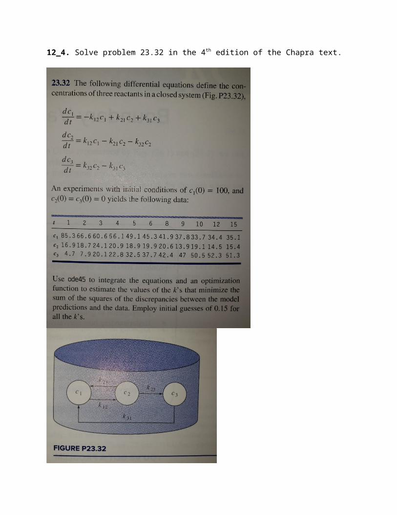
dc1dt = -k12*c1 + k21*c2 + k31*c3;dc2dt = k12*c1 - k21*c2 - k32*c2;dc3dt = k32*c2 - k31*c3; %RecombinedCdt = [dc1dt; dc2dt; dc3dt];end function SSE = sumsquares(k,t_obs,C_obs,C0)%This will run the ODE function for a given k value (to be manipulated by%fminsearch) and return the corresponding sum of squared errors.%Note: we can tell ode45 to run only at the t_obs values for comparison.%Also have to include 0, since that's where our initial conditions are.[t,C] = ode45(@ps12_4_func,t_obs,C0,[],k);%Compare C_obs with C SSE = sum(sum((C-C_obs).^2));end

Output:

k12 =

0.2030

k21 =

0.1103

k31 =

0.0973

k32 =

0.4160

Challenge 12_5 (4 points extra credit)

We’re firing a cannon to land a projectile within a target zone. We define a coordinate system in which y is the direction toward the target zone (positive direction moves from us toward the target), x is the “left/right” direction when facing the target zone (positive direction to the right), and z is the direction normal to the ground (positive direction upward).

The movement of the projectile is governed by the following equations of motion:

dxdt

=v xdydt

=v ydzdt

=v z

d vx

dt=ax

d v y

dt=a y

dzdt

=az

The accelerations can be defined by the following force balances:

ax=[ sign (vwind , x−vx ) ] Cd

2ρair (vwind ,x−v x)

2 A ref /mball

a y=[ sign (vwind , y−v y) ]Cd

2ρair (vwind , y−v y )2 A ref /mball

az=[sign (vwind , z−vz ) ]Cd

2ρair (vwind , z−vz )

2 A ref /mball−g

Note the “sign” function, which can be used in MATLAB. This returns a (+1) or a (-1); this comes from air resistance opposing the direction of movement.

The appropriate Aref value for a sphere’s surface area is calculated as:

Aref =π4Dball

2

For this problem, we consider the following physical constants:

Cd=0.47 ρair=0.737 kgm3 Dball=0.254m mball=45kg g=9.81 m

s2

We also consider the following initial position of the projectile:

x (t=0 )=0 y (0 )=0 z (0 )=0

The initial velocities are determined by the following equations, as determined by the launch angles of the cannon:

vx ( 0 )=v0sin (ϕ ) cos (θ ) v y (0 )=v0 sin (ϕ ) sin(θ) vz (0 )=v0 cos (ϕ)

For this problem, v0 is fixed at 142 m/s.

The target zone is located in a 10x10 square landing area defined by coordinates:

(−10,1370,60 ) ; (10,1370,60 ); (−10,1430,60 ); (10,1430,60)

(A)First consider the case in which vwind , x=0 and θ=90 °. (This corresponds to the case in which all x-components are 0.) Assume vwind , z=0. For each of the following cases, find a value of ϕ for which the projectile will land in the target zone.

a. vwind , y=0 ms

b. vwind , y=−20ms (wind in your face)

c. vwind , y=30 ms

(B) There’s now a strong cross wind: vwind , x=−30, vwind , y=−10, vwind , z=0. Find a pair of θ and ϕ such that your cannon will hit its target zone.