,1)250(6 7e&1,&26 0,'( 8& 7(&+1,&$/ 5(32576 0,'(...
TRANSCRIPT

INFORMES TÉCNICOS MIDE UC / TECHNICAL REPORTS MIDE UC
IT1006
JORGE MANZI, ERNESTO SAN MARTÍN, SÉBASTIEN VAN BELLEGEM
School System Evaluation by Value-Added Analysis under Endogeneity
Centro de Medición MIDE UC / Measurement Center MIDE UC

School System Evaluation by Value-Added Analysis underEndogeneity
JORGE MANZI1, ERNESTO SAN MARTIN1,2, SEBASTIEN VAN BELLEGEM3
1Measurement Center MIDE UC, Pontificia Universidad Catolica de Chile, Chile.2Department of Statistics, Pontificia Universidad Catolica de Chile, Chile.
3CORE, Louvain-la-Neuve, Belgium & Toulouse School of Economics, France
July 8, 2010
Abstract
Value-added analysis is a common tool in analysing school performances. In this paper, we anal-yse the SIMCE panel data which provides individual scores of about 200,000 students in Chile, andwhose aim is to rank schools according to their educational achievement. Based on the data col-lection procedure and on empirical evidences, we argue that the exogeneity of some covariates isquestionable. This means that a nonvanishing correlation appears between the school-specific effectand some covariates. We show the impact of this phenomenon on the calculation of the value-addedand on the ranking, and provide an estimation method that is based on instrumental variables in orderto correct the bias of endogeneity. Revisiting the definition of the value-added, we propose a newcalculation robust to endogeneity that we illustrate on the SIMCE data.
Keywords: Value-added, School effectiveness, Multilevel model, Endogeneity, Instrumental vari-ables.
1 Introduction
A typical way to measure the school performance is to compare the progress that students make betweentwo or more test occasions. Among the numerous measurement methods, the “value-added analysis” hasoften been considered in empirical studies (see e.g. OECD, 2008, and the references therein). The value-added analysis aims at measuring the gain (or the loss) of beeing in a given school with respect to anaverage school. This average school is defined as the average performance of the schools that are found inthe data set, and therefore the value-added provides a data-driven measure of school efficiency. Anotheraspect of the value-added analysis is that it usualy controls for a set of variables such as individualcharacteristics (e.g. students gender or socio-economic level) or school/environmental characteristics.Moreover, the previous attained score of the students is always considered as a control variable.
Measuring the value-added requires an appropriate model for the test score. Due to the hierarchicalstructure found in educational data sets, the multilevel generalized linear model is used routinely in this
1
analysis. In the statistical parlance, the value-added in this model is calculated as the predictor of therandom school-effect of the multilevel regression (Raudenbush and Willms, 1995; Tekwe et al., 2004).
The recent literature however has shown that systematic bias problems occur in the inference for themultilevel model on educational data. A typical source of bias is due to omitted variables (Kim and Frees,2006; Lockwood and McCaffrey, 2007). The reason may be explained as follows. We have recalled thatthe multilevel regression model used in the value-added analysis contains the prior attainment score as aregressor. Suppose that a variable is omitted in this model and this variable is correlated with both theactual test score and the prior test score. Because the variable is omitted, it is therefore included in theerror term of the multilevel model. Therefore, the error of the model is not uncorrelated with the priorattainment score. This correlation is a source of bias in the standard estimation for regression model, andis sometimes called an endogeneity bias (Halaby, 2004; Steele et al., 2007; Spencer, 2008).
The last argument will be extensively described and discussed in this paper. It has an important impacton the inference for multilevel models because it is not obvious to understand which variable is omittedor, if so, it is not always easy to measure this omitted variable. For instance, the school effect is by defi-nition unobserved and is influential on both the previous attainment score and the actual score, providedthat the student has not switched schools between the two tests. In more technical terms, there is a nonvanishing correlation between the random school-effect and the prior attaintment score as soon as thestudent has already been “treated” by its school at the time of the first test occasion. This shows why theendogeneity bias is systematic when there is little movement of students between test occasions.
The literature contains some methods of estimation to circumvent the endogeneity bias in multilevelmodels. Two major contributions are Ebbes et al. (2004) and Kim and Frees (2007), and we also cite therecent work of Grilli and Rampichini (2009) in the context of general measurement errors. The presentpaper aims to study the impact of the endogeneity on the measure of the value-added. We show that, inthe presence of endogeneity, an additive correcting term must be applied on the usual calculation of thevalue-added indicator of a school. We provide the exact form of the correction term and show how tocalculate it from data.
Our methodology is motivated and illustrated by the study of the Chilean school performance. Arich dataset is used in which the score in mathematics and other covariates of 163,286 students from1,886 schools were measured in 2004 and 2006. A description of the Chilean educational system andof the research on school effectiveness in that country is to be found in Section 2 below. In Section 3,the dataset is described. Section 4 starts with a structural definition of the value-added and shows theresult of a value-added analysis under standard assumptions (e.g. under exogeneity of all covariates). InSection 4.3, we argue that the endogeneity of some covariates is not avoidable and we describe the impactof this endogeneity on the value-added. The calculated value-added may be used in order to rank schoolsaccording to their performance. We show what is the impact of the endogeneity on the school ranking.In Section 4.4, we demonstrate how the value-added has to be corrected, and we show the impact of thiscorrection on the value-added of the 1,886 chilean schools. A formal definition of the multilevel modelunder endogeneity is also presented in the Appendix. The appendix describes the steps that are used inorder to calculate the value-added under endogeneity.
2
2 Chilean Educational System and School Effectiveness Research
2.1 The SIMCE test
One of the most important aspects in the development and achievements of a country is having a satis-factory educational system that is accessible to all, or the big majority, of its individuals. In Chile, it iswidely acknowledged that the state of its educational system is a hindrance to its development. A keyaspect that has been criticized is the poor quality of some school teachers with limited knowledge ofthe material that they need to teach. Another aspect is the inequality between public schools and privateschools (see OECD, 2007). However during the last decades Chile has worked to improve the quality ofits education leading to the generation of novel public policies to tackle a part of the problems. Someexamples are the increase in the amount of time that students should spend at school, and a new lawstating that it is mandatory that all students get education for the four years that correspond to secondaryeducation. The Preferential Subsidy Law (passed by the Senate on May 4, 2009) is another example.Broadly speaking, this new law fixes conditions to evaluating students’ performance and, based on them,to classify schools into three types: charter school, emerging school, and recovery school. Economicaland administrative support are provided to schools according to that classification.
With the aim of uncovering the possible causes of deficiency in the educational system, the Chileangovernment has been systematically gathering data since 1988 about students’ performance. This largescale data collection is known as the SIMCE test (SIMCE stands for Sistema de Medicion de Calidadde la Educacion). This policy is consistent with what the Organization for Economic Co-operation andDevelopment (OECD) has found to be the first step to unveil the problems in the educational system(OECD, 2008). Together with the national voucher system, a national evaluation of student performancewas conceived that would provide parents with necessary information to make decisions about schools.In 1988, students in all Chilean schools begun to be tested with the SIMCE test, which was given inalternating years in 4th and 8th grade, and later in 1994, also in 10th grade. Since 2005, the SIMCE testwas applied all the years to 4th grade. Until 1994, SIMCE results were delivered only in aggregates, theywere given only to schools and Municipalities, and were not comparable for different years. Startingin 1995, the SIMCE results by schools begun being publicized through the media, with the aim ofcontributing to its original purpose of providing information for parents to make decisions about schools.
In 1998, SIMCE suffered several changes. First, an effort was made to tightly tie the SIMCE testsinto the educational goals and contents specified in the new national curricula defined by the ChileanMinistry of Education. Together with this, the instruments were modified to include not only multiplechoice questions, but also open questions devoted to test more complex skills such as critical thinkingor written expression. The complementary questionnaires for parents and school principals were alsomodified in order to collect better quality information at the individual level. In 2000, results of theSIMCE started to be published by group of schools having a comparable socioeconomic status, in orderto facilitate comparisons between schools that educate similar students. With the aim to improve thequality of teaching, the government also asked to provide example of questions and solutios in the finalreport of the SIMCE test given to schools. For an example of a SIMCE report, see SIMCE (2009).
With regards to the instruments themselves, Item Response Theory methodology has been introducedin 2000, allowing comparisons across years, and making it possible to produce more accurate descrip-tions of different levels of performance, to measure with precision students with different skill levels,
3

and to examine possible item bias. For details, see SIMCE (2008).Taking into account the calendar of the SIMCE applications, it is possible for each student to obtain
two measures of their educational performance. Most of these measurements will be taken every fouryears; for instance, students who were measured in 2005, were still measured in 2009 when they werein the 8th grade. In the study reported in this paper, we considered students who were measured in 2004(when they were at the 8th grade) and in 2006 (when they were at the 10th grade).
2.2 The Chilean educational system
The Chilean education system has suffered several changes in the last three decades. In 1980, elementsof privatization and decentralization were introduced through a massive voucher system by which pri-vate schools were allowed to receive a state subsidy proportional to the number of students attendingclasses, as long as they met certain requirements. At the same time, administration of public schools wasshifted from the Ministry of Education to local authorities (Municipalities). Up to 1980, the Ministry ofEducation was in charge of financing public education, establishing educational contents and investingin infrastructure. After the 1980’s reform, the Ministry retained authority over educational contents andgoals, and it was responsible for supervising the functioning of schools receiving voucher monies, whileinfrastructure and hiring decisions were delegated to local school administrators, both public and pri-vate. As a consequence of the introduction of private operators into the system, a new group of schoolswas created – private-subsidized schools – and this increased the number of schools significantly in lateryears.
From 1990, a significant increase in public investment in education was registered. This increase ininvestment had a clear impact on education coverage. According to Bellei (2005), between 1990 and2000 this raised coverage in primary education from 93% to 98% and from 74% to 85% in secondaryeducation. However, increases in educational quality, as measured by standardized tests, were not evi-dent. It is likely that the increases in education coverage in those years have actually lowered averagetest scores, as children who would otherwise have been outside the school system begin to enter school.In spite of this, test scores have not experienced a drop. For example, in 2003 there was a 20% incrementover the previous year in the number of students taking the national SIMCE tests, but average SIMCEscores did not drop significantly.
In 1991, the “Estatuto Docente” was created, establishing regulations for teacher salaries and protectingthem from being fired from the Municipal system, tending to make the system more rigid. Also in1991, a number of improvement programs were put in place that targeted schools which cater to themost vulnerable students. In 1993 shared financing is introduced, which allowed private-subsidized andsecondary public schools to charge parents a fee in addition to the state voucher, provide that this feedoes not exceed a certain value. Primary public schools can not use this system, and secondary publicschools can charge a fee only with the agreement of the majority of parents in the school.
The Chilean schools are accordingly grouped into four groups: Public I schools are financed by thestate and administered by county corporations, whereas Public II schools are also financed by the state,but administered by county governments; Subsidized schools are financed by both the state and parents,and administered by the private sector; Private schools are fee-paying schools that operate solely onpayments from parents and administered by the private sector.
4

2.3 School effectiveness research in Chile
Chilean researchers have undertaken qualitative effectiveness research particularly on schools in poverty.Among the research reports on school effectiveness based on SIMCE data, the two mostly influentialworks are Bellei et al. (2004) and Eyzaguirre (2004). One aim in Bellei et al. (2004) is to characterizeefficient schools. The method used in this report classifies schools according to an average of the SIMCEscores. One aim of Eyzaguirre (2004) was to study the factors of performance for the schools that areconsidered to have the lowest socio-economic level. However, sampling procedures were misleading,which probably led to the author to conclude (challenging most international literature) that ’this evidenceshows that education in poverty does not differ essentially from the education of pupils located in othercontexts’ (Eyzaguirre, 2004, p.259).
The Chilean government has recently funded several studies on school effectiveness based on theSIMCE data set. Between 2007 and 2009, the SIMCE office (from the Ministry of Education) com-missioned three value-added studies, using the SIMCE data sets: a national value-added study with the2004 and 2006 SIMCE applications (del Pino et al., 2008) and two value-added analysis at the Metropoli-tan Region level (del Pino et al., 2008, 2009). These studies were relevant not only for being the firstnational value-added analysis performed in Chile with governmental support, but also by showing thatthe ranking of schools obtained by value-added indicators are dramatically different from the rankingobtained by averaging the SIMCE scores. From a political point of view, these results provide a moretransparent way to compare school efficiency in Chile.
Another example is the study ordered by the Ministry of Education of the Chilean government, dealingwith the determination of standards for learning in the Chilean educational system (Paredes et al., 2010). The context of this study was the Preferential Subsidy Law above-mentioned. One of the objectivesof the study was to identify specific factors explaining students performance as measured by the SIMCEtest. The main objective was to use this information to estimate school effectiveness and thus to obtainschool classification into the three categories mentioned above (charter school, emerging school andrecovery school). Another related study commanded by the government was the classification of schoolswith the purpose of distributing resources to more vulnerable schools (Marshall et al., 2008).
It should be mentioned that the aforementioned studies and many others are expected to guide some as-pects of the implementation of a new law, called Ley General de Educacion (General Law of Education),that is nowadays being discussed by the Parliament. This law requires the creation of an agency, theNational Agency for School Quality, which will be in charge of measuring the quality and achievementsof schools.
3 Data description
3.1 The 2004 and 2006 SIMCE applications
The dataset used in this study correspond to the 2004 and 2006 cross sections of the SIMCE test in thefield of Mathematics. In 2004, the test was applied to 276,365 students from the 8th level. In 2006 mostof the tested students were at the 10-th level. Using the unique national identity card, it was possible tolink both cross sections at the student level, obtaining thus a panel of 177,463 students over two periodsof time. We also limited the data set in considering schools with at least 20 students. The final dataset
5
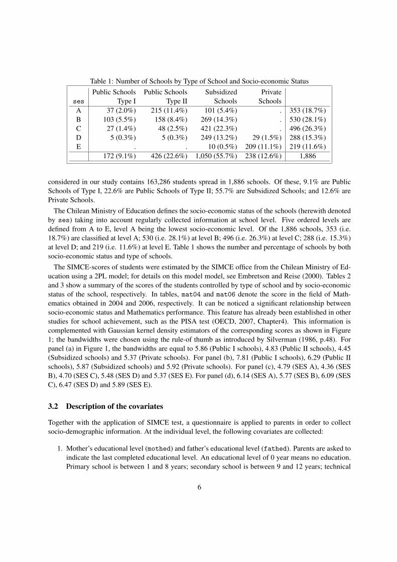
Table 1: Number of Schools by Type of School and Socio-economic StatusPublic Schools Public Schools Subsidized Private
ses Type I Type II Schools SchoolsA 37 (2.0%) 215 (11.4%) 101 (5.4%) . 353 (18.7%)B 103 (5.5%) 158 (8.4%) 269 (14.3%) . 530 (28.1%)C 27 (1.4%) 48 (2.5%) 421 (22.3%) . 496 (26.3%)D 5 (0.3%) 5 (0.3%) 249 (13.2%) 29 (1.5%) 288 (15.3%)E . . 10 (0.5%) 209 (11.1%) 219 (11.6%)
172 (9.1%) 426 (22.6%) 1,050 (55.7%) 238 (12.6%) 1,886
considered in our study contains 163,286 students spread in 1,886 schools. Of these, 9.1% are PublicSchools of Type I, 22.6% are Public Schools of Type II; 55.7% are Subsidized Schools; and 12.6% arePrivate Schools.
The Chilean Ministry of Education defines the socio-economic status of the schools (herewith denotedby ses) taking into account regularly collected information at school level. Five ordered levels aredefined from A to E, level A being the lowest socio-economic level. Of the 1,886 schools, 353 (i.e.18.7%) are classified at level A; 530 (i.e. 28.1%) at level B; 496 (i.e. 26.3%) at level C; 288 (i.e. 15.3%)at level D; and 219 (i.e. 11.6%) at level E. Table 1 shows the number and percentage of schools by bothsocio-economic status and type of schools.
The SIMCE-scores of students were estimated by the SIMCE office from the Chilean Ministry of Ed-ucation using a 2PL model; for details on this model model, see Embretson and Reise (2000). Tables 2and 3 show a summary of the scores of the students controlled by type of school and by socio-economicstatus of the school, respectively. In tables, mat04 and mat06 denote the score in the field of Math-ematics obtained in 2004 and 2006, respectively. It can be noticed a significant relationship betweensocio-economic status and Mathematics performance. This feature has already been established in otherstudies for school achievement, such as the PISA test (OECD, 2007, Chapter4). This information iscomplemented with Gaussian kernel density estimators of the corresponding scores as shown in Figure1; the bandwidths were chosen using the rule-of thumb as introduced by Silverman (1986, p.48). Forpanel (a) in Figure 1, the bandwidths are equal to 5.86 (Public I schools), 4.83 (Public II schools), 4.45(Subsidized schools) and 5.37 (Private schools). For panel (b), 7.81 (Public I schools), 6.29 (Public IIschools), 5.87 (Subsidized schools) and 5.92 (Private schools). For panel (c), 4.79 (SES A), 4.36 (SESB), 4.70 (SES C), 5.48 (SES D) and 5.37 (SES E). For panel (d), 6.14 (SES A), 5.77 (SES B), 6.09 (SESC), 6.47 (SES D) and 5.89 (SES E).
3.2 Description of the covariates
Together with the application of SIMCE test, a questionnaire is applied to parents in order to collectsocio-demographic information. At the individual level, the following covariates are collected:
1. Mother’s educational level (mothed) and father’s educational level (fathed). Parents are asked toindicate the last completed educational level. An educational level of 0 year means no education.Primary school is between 1 and 8 years; secondary school is between 9 and 12 years; technical
6

100 200 300 400
0.00
00.
002
0.00
40.
006
0.00
80.
010
2004−scores
Den
sity
est
imat
ion
Public IPublic IISubsidiezedPrivate
(a)
100 200 300 400
0.00
00.
002
0.00
40.
006
0.00
80.
010
2006−scores
Den
sity
est
imat
ion
Public IPublic IISubsidiezedPrivate
(b)
100 200 300 400
0.00
00.
002
0.00
40.
006
0.00
80.
010
2004−scores
Den
sity
est
imat
ion
ABCDE
(c)
100 200 300 400
0.00
00.
002
0.00
40.
006
0.00
80.
010
2006−scores
Den
sity
est
imat
ion
ABCDE
(d)
Figure 1: Gaussian kernel density estimators for the 2004- and 2006-scores distributions
7

Table 2: SIMCE Mathematics performance by Type of School
Type of Number of Mean S.D. Mean S.D.School Students mat06 mat06 mat04 mat04
Public Schools I 22,799 (14.0%) 245.8 64.6 253.5 48.5Public Schools II 50,918 (31.2%) 241.8 61.1 251.1 46.9Subsidized Schools 77,314 (47.3%) 263.5 61.9 264.7 47.0Private School 12,255 (7.5%) 331.7 47.1 315.4 40.8
Table 3: SIMCE Mathematics performance by School Socioeconomic Status
ses Number of Mean S.D. Mean S.D.Students mat06 mat06 mat04 mat04
A 29,369 222.5 53.4 236.3 41.6B 60,143 237.2 57.9 247.3 43.8C 43,600 274.3 57.3 272.9 44.2D 18,649 308.3 53.9 296.7 43.5E 11,525 333.7 45.7 316.8 40.3
secondary school is 13 years; technical professional school is 14 or 15 years; incomplete universityeducation is 16 years; complete university level is 17 years; master level is 18 years; and PhD levelis 19 years.
2. Student school movement indicator (move). This is a categorical variable indicating whether astudent moved from a school to another school between 2004 and 2006. As Table 4 shows, 70% ofstudents moved between 2004 and 2006. This mobility is due in part to the fact that most schoolsattended by students at 2004 organized studies at the primary level only. Therefore those studentswere obliged to change school between the two periods of testing.
3. Student fall indicator (fall). This is a categorical variable, which indicates whether a student hasfall in the past before 2006.
4. Gender.
At the school level, the following covariables were available:
1. Socio-economic status of the school (ses) (above-described).
2. Selectivity of the school (select). A selectivity mechanism widely used by schools is the selec-tivity by ability. In their questionnaire, parents are asked whether a test of knowledge on theirchild was organized when they applied for the school. Schools which use this mechanism of se-lection are free to decide whom to apply such a test. For each school, select corresponds to theproportion of questionnaires which report the application of such a mechanism.
8

Table 4: Student school movement between 2004 and 2006Type of Percentage of Mean S. D. Mean S. D.
move School students mat06 mat06 mat04 mat04
No Public Schools I 2,904 (1.8%) 260.4 72.8 265.2 55.9Public Schools II 5,799 (3.6%) 265.3 72.5 269.1 55.8
Subsidized Schools 29,907(18.3%) 280.4 60.0 276.0 46.4Private School 10,320 (6.3%) 334.2 45.8 317.7 40.1
Yes Public Schools I 19,895 (12.2%) 243.7 63.0 251.8 47.0Public Schools II 45,119 (27.6%) 238.7 58.8 248.7 45.1
Subsidized Schools 47,407 (29.0%) 252.9 60.8 257.6 45.9Private School 1,935 (1.2%) 318.3 51.1 303.2 42.4
4 Statistical Analysis by Instrumental Mixed Modeling
4.1 A Definition of the value-added
Since our database contains two cross-sections, a possible approach to measure the efficiency of schoolsis to compute their so-called value-added. Value-added measures the gain (or loss) of being in a givenschool and is based on the student progress. It therefore requires at least one lagged measure of the scorerepresenting a baseline. Progression of students in each schools are then compared jointly, that is thegain (or loss) of being educated in a given school is calculated with respect to an “average” school; seeRaudenbush and Willms (1995); Raudenbush (2004) and OECD (2008, pp.16-17).
In order to formalize that notion we denote by mat06ij the observed score in mathematics in 2006for pupil i belonging to school j, and by mat04ij the lagged score in 2006. All other covariates, beingschool-specific or not, are denoted by the vector Xij . In addition to those covariates, we also have thepossibility to control for the school selectivity by adding other covariates. A natural candidate is to takethe average of mat04ij over students in each school j as a possible control variable. That variable isbelow denoted by avmat04j and will be showed to satisfactorily control for the unobserved selectivityprocess of schools.
The random effect of school j is denoted by θj . By definition this latent variable controls for school-heterogeneity and thus represents unobserved school-specific characteristics that may include both schoolpractices (on which school have some control) and school contexts (Raudenbush, 2004). With thesenotations, the value-added is the measure of the following difference :
VAj =1
nj
nj∑i=1
E(mat06ij | mat04ij , avmat04j ,XXXij , θj) −
(1)
1
nj
nj∑i=1
E(mat06ij | mat04ij , avmat04j ,XXXij),
where nj is the number of pupils belonging to school j. The first term is the average of the expectedscores given the specific characteristics of school j when controlling for the lagged score, the selectivity
9

and all other covariates. The second term integrates out the school-specific effect and therefore representsthe average of expected scores of an average school given the covariates.
The practical computation of these expectations are based on a specific model that must be assumedon the score. Hierarchical linear mixed (HLM) models appear to be a widely used standard in the topicof educational assessment. It assumes the following specification:
mat06ij = X ′ijβ + γmat04ij + αavmat04j + θj + ϵij , (2)
where β is a vector of parameter (we have modeled the intercept as the first element of β), γ is theparameter of the lagged score, and ϵij are independent errors, possibly heteroscedastic and often assumedto be zero-mean and normally distributed. If the school random effect θj is supposed to be independentfrom ϵij and from all covariates of the model, then the expectation E(θj | mat04ij , avmat04j ,XXX ij)vanishes and we find that
VAj = θj
(3)
= E(mat06ij | mat04ij , avmat04j ,XXX ij , θj)− E(mat06ij | mat04ij , avmat04j ,XXXij)
for all i; that is, the value-added of school j is given by the random effect θj . This equality makesexplicit the structural meaning of the random effect θj and actually explains why and in which senseit is a representation of the value-added of school j. In this setting, the value-added is computed asthe predictor of the random effect, as typically done in this type of literature; see e.g. Raudenbush andWillms (1995); Goldstein and Spiegelhalter (1996); Goldstein and Thomas (1996); Tekwe et al. (2004);Hutchison et al. (2005).
4.2 Results from a standard valued-added analysis
In a preliminary analysis, a homoscedastic HLM model has been fitted to the SIMCE data. However,after residual analysis controlling by the socio-economic status of the schools, it was concluded thatthe normality assumption of the random effect is violated. We therefore run the valued-added analysisby fitting a heteroscedastic HLM models in which the variance of θj and ϵij may depend on the socio-economic level of the school. More specifically, the variance structure in (2) is supposed to be suchthat
V ar(Yij | mat04ij , avmat04j ,XXX ij , θj) = σ2ρ(j) for all students i belonging to school j,
V ar(θj | mat04ij , avmat04j ,XXXij) = τ2ρ(j),
where ρ is a function that maps j into the socioeconomic status of school j; that is, ρ(j) = A if the socio-economic status of the school j is A, and so on. In agreement with this structure, the conditional modelof Yij given mat04ij , avmat04j ,XXX ij and θj was specified with an intercept for each socio-economiclevel using the covariate ses.
The initial within-variances are τ2A = 1, 313.1; τ2B = 1, 109.3; τ2C = 1, 412.2; τ2D = 3, 586.1; andτ2E = 7, 388.4; and the initial between-variances are σ2
A = 2, 433.9; σ2B = 2, 515.9; σ2
C = 2, 411.4;σ2D = 2, 202.2; σ2
E = 1, 831.1. Once it is controlled by the baseline score mat04, along with an
10

intercept by each socio-economic level, both the within and between variances decrease dramatically.Nine specifications were fitted and are summarized in Table ??. The reference for ses is the socio-economic status A; the reference for fall is “the student fells in the past”; the reference for move is “thestudent did move between 2004 and 2006”; and the reference for sex is “woman”.
As we mentionned above, the covariate avmat04 is a relevant control variable for the unobservedselectivity of schools. By “unobserved” selectivity, we refer to a selectivity bias that is not self reportedby the parents through the covariate select. We now give empirical arguments supporting that choice.
First, we show the existence of a selectivity bias in the sample. For this, we can compare the value-added obtained from HLM models that do not contain select with the value-added that is obtained whenwe add this covariate. In Tables 5 6, we therefore compare HLM0 with HLM0b, HLM1 with HLM1b andso on. The five pictures of Figure 2 show the comparison of the value-added for the five HLM models. Inthe plot, value-added in black color correspond to schools that are such that select > 50%, that is, theyhave a high reported selectivity. Red value-added are the other schools, having a low reported selectivity.In general, these figures show that highly selective schools (in black) have higher value-added if selectis not included in the HLM model. Conversely, the value-added of less selective schools (in red) havelower value-added if select is not included in the model. Consequently, the exclusion of select asa covariate benefits the schools which select at least 50% of the students; and the inclusion of selectbenefits the schools which select at most 50% of the students.
To see now how avmat04 helps in controlling the selectivity bias, compare pictures (b) to (e) in FigureFigure 2. We see that the inclusion of avmat04 as a covariate decreases the distance between thesetwo types of schools and, therefore, the inclusion/exclusion of select as a covariate is successfullycontrolled. The same conclusions can be drawn if the comparisons are done between schools of the sametype (namely, public schools type I; type II; subsidized; and private).
11

HL
M0
HL
M0b
HL
M1
HL
M1b
HL
M2
HL
M2b
HL
M3
HL
M3b
HL
M4
HL
M4b
HL
M5
Inte
rcep
t24
7.5∗
227.
7∗21
8.8∗
215∗
93.2
∗10
2.1∗
213.
9∗21
0.2∗
90.0
∗98
.6∗
100.
8∗(0
.9)
(0.8
)(0
.8)
(0.9
)(4
.6))
(4.8
)(0
.9)
(0.9
)(4
.8)
(4.8
)(3
.1)
mat04
0.83
∗0.
83∗
0.81
∗0.
8∗0.
8∗0.
8∗0.
81∗
0.8∗
0.8∗
0.8∗
0.8∗
(0.0
02)
(0.0
02)
(0.0
02)
(0.0
02)
(0.0
02)
(0.0
02)
(0.0
02)
(0.0
02)
(0.0
02)
(0.0
02)
(0.0
02)
ses
B6.
1∗3.
8∗5.
7∗3.
5∗-0
.46
-0.8
14.
3∗2.
1-1
.7-2
.1(1
.2)
(1.1
)(1
.2)
(1.1
)(0
.9)
(1.0
)(1
.1)
(1.2
)(1
.0)
(1.0
)
ses
C21
.6∗
16.4
∗20
.1∗
15.1
∗1.
20.
8717
.2∗
12.4
∗-1
.3-1
.7(1
.2)
(1.2
)(1
.2)
(1.2
)(1
.2)
(1.2
)(1
.2)
(1.2
)(1
.2)
(1.2
)
ses
D36
.3∗
28.9
∗34
.5∗
27.4
∗4.
0∗3.
7∗30
.4∗
23.4
∗0.
30.
1(1
.2)
(1.3
)(1
.2)
(1.3
)(1
.6)
(1.5
)(1
.2)
(1.3
)(1
.5)
(1.5
)
ses
E46
.4∗
37.2
∗44
.2∗
35.3
∗0.
941.
139
.0∗
30.3
∗-3
.5-3
.4(1
.1)
(1.3
)(1
.2)
(1.3
)(1
.9)
(1.9
)(1
.2)
(1.3
)(1
.9)
(1.9
)
fall
12.4
1∗12
.4∗
12.4
∗12
.4∗
12.1
∗12
.0∗
12.0
∗12
.0∗
12.0
∗(0
.32)
(0.3
)(0
.3)
(0.3
)(0
.3)
(0.3
)(0
.3)
(0.3
)(0
.3)
move
2.68
∗2.
7∗2.
5∗2.
6∗2.
4∗2.
4∗2.
2∗2.
3∗2.
2∗(0
.3)
(0.3
)(0
.3)
(0.3
)(0
.3)
(0.3
)(0
.3)
(0.3
)(0
.3)
sex
4.1∗
4.1∗
4.0∗
4.0∗
4.0∗
4.0∗
4.0∗
4.0∗
4.0∗
(0.2
)(0
.2)
(0.2
)(0
.2)
(0.2
)(0
.2)
(0.2
)(0
.2)
(0.2
)
fathed
0.32
∗0.
32∗
0.32
∗0.
32∗
0.31
∗(0
.04)
(0.0
4)(0
.03)
(0.0
3)(0
.03)
mothed
0.37
∗0.
37∗
0.37
∗0.
37∗
0.36
∗(0
.04)
(0.0
4)(0
.04)
(0.0
4)(0
.03)
avmat04
0.54
∗0.
49∗
0.53
∗0.
49∗
0.47
∗(0
.019
)(0
.02)
(0.0
2)(0
.02)
(0.0
1)
select
18.0
∗17
.5∗
6.7∗
17.2
∗6.
5∗6.
5∗(1
.3)
(1.3
)(1
.3)
(1.3
)(1
.2)
(1.2
)
AIC
1,63
9,13
41,
638,
954
1,63
7,23
11,
637,
056
1,63
6,62
51,
636,
593
1,63
6,89
21,
636,
722
1,63
6,29
81,
636,
268
1,63
6,28
9
Tabl
e5:
Res
ults
from
clas
sica
lVal
ue-A
dded
anal
ysis
12

HL
M0
HL
M0b
HL
M1
HL
M1b
HL
M2
HL
M2b
HL
M3
HL
M3b
HL
M4
HL
M4b
HL
M5
τ2 A
202.
418
9.6
197.
818
4.1
153.
714
9.0
195.
918
3.5
153.
614
9.2
149.
9τ2 B
363.
931
8.2
348.
130
7.0
207.
420
5.0
343.
330
2.9
206.
720
4.2
206.
1τ2 C
342.
030
0.2
335.
529
5.0
199.
819
6.4
330.
929
2.0
198.
719
5.5
195.
8τ2 D
207.
018
6.5
201.
318
2.4
151.
615
1.5
202.
118
3.5
152.
315
2.2
153.
9τ2 E
117.
511
7.4
117.
011
7.0
142.
113
6.4
117.
311
7.5
142.
413
6.9
136.
8σ2 A
1372
.313
72.2
1347
.913
47.8
1347
.613
47.5
1345
.613
45.5
1345
.213
45.2
1345
.2σ2 B
1391
.013
91.0
1373
.113
73.1
1373
.113
73.1
1368
.513
68.5
1368
.513
68.5
1368
.5σ2 C
1289
.412
89.5
1278
.512
78.5
1278
.812
78.8
1277
.312
77.3
1277
.612
77.6
1277
.6σ2 D
1192
.311
92.3
1184
.211
84.2
1184
.011
84.0
1183
.211
83.3
1183
.011
83.1
1183
.1σ2 E
934.
393
4.2
928.
592
8.4
927.
792
7.8
926.
392
6.2
925.
692
5.6
925.
6
Tabl
e6:
Res
ults
from
clas
sica
lVal
ue-A
dded
anal
ysis
13

The fixed effects corresponding to the covariates at the individual level are stable across the differentmodels (when the covariate is included): around 0.8 for mat04; around 12.0 for fall (the coefficientis positive for students who did not fall in the past); around 2.2 for move (the coefficient is positive forstudents who did not move between 2004 and 2006); around 4.0 for sex (the coefficient is positive formen); around 0.32 for fathed and 0.37 for mothed.
With respect to the fixed effects at the school level, the coefficient of select is around 17.0 whenavmat04 is not included in the model; when it is included, the coefficient of select is around 6.5,whereas the coefficient of avmat04 is around 0.50. This also quantifies how avmat04 controls the selec-tivity of the school. With respect to the socio-economic level of the school, the type III test (computedby PROC MIXED of SAS) is significative in all models. Furthermore, when the t-test correspondingto each category of ses is significant, the fixed effect for level B is between 3.5 and 6.1; for level Cbetween 12.4 and 21.6; for level D, between 23.4 and 36.3; and for level E, between 30.3 and 46.4.However, when avmat04 is included in the model (in HLM2, HLM2b, HLM4 and HLM4b models),some (if not all) of the categories of ses are non significant. Taking into account the AIC-criterion, themodel HLM4b is the best model although the four categories of ses are non significant.
From the above analysis, we keep model HLM5 as the baseline for the following steps of our analysisbelow.
4.3 The endogeneity of some covariables
Although the previous analysis follows a classical approach to compute the value-added, our descriptionabove emphasizes that it relates to structural assumptions, among which the most critical is certainly theindependence between the random effect θj and all covariates.
Recall that mat04ij represents the lagged version of the score and avmat04j denotes its average overschools. It is likely that these two covariates already contain the effect of the school, particularly if stu-dent i already belongs to school j at that time. Independence between the school effect θj and variablesmat04ij or avmat04j is therefore questionable, and it raises the important statistical question of whatcorrections on the value-added calculation should we apply if this assumption is not fulfilled.
It is possible to support this observation from the SIMCE data. Over all students kept in the database,70% have moved between 2004 and 2006. The reason of moving may be due to the choice of the parents,or may be unavoidable due to the school system itself. Let us consider the HLM model and the value-added of schools that are calculated from the subsample of moving students only. In Figure 3 we comparethis value-added with the value-added that is calculated from the whole sample. Both calculations arebased on the HLM5 specification. A high variation is observed between the two calculations, leadingto important differences in the school ranking. To quantify that last point, we notice that the Spearmancorrelation between the two value-added predictions is 0.873.
To have a better picture of what happened, it is useful to compare this difference according to theschool type. As we can observe from the above Table 4, the moving rate is variable according to thetype of school considered: it is 16% for Private Schools, 61% for Subsidized Schools, 87% for PublicSchools Type II and 89% for Public Schools Type I. From Figure 4 we see that the highest variability areobserved for subsidized and private schools. Although that change is not apparent on average for publicschools, noticeable differences are observed for some of them. Again the Spearman correlation provides
14

+
+++
+
+
+
+
+++
+
+ ++
+
+
+
+
+
+
+
++
+++
++++
+
+
++
++
++
++
++
++
+
+
+
+
++
+
+
++
+
++
++
+
+
+
++
+
+
++
+
++
+
+
+
+++
++
+
+
+++
++ ++
+
+
+
+
+
+
+
+++
+
+++
++
+
+++
+++
++
+
+
+
+
+++
+
+
++
++
++
+
+
++
+
+
++++
++
+
+
+
+++
+
+
+
+
+
++
+
+
++
+
++
+
+
++
++
+
++
+
+
+
+
++
+
+
+
+
+
+
+++
+
+
+
+
++
+
+
+
+
++
+++++
++
++
+
+
+
+
++++
++
++
+++
+
++
+
++
++
+
+
+
++
+
++++
+
+
+
+
+
+
++
+
++
++
+
++++
++
+
++
+
+ ++
+
+
+
+++
+
+
++
+
+
+
+
++
+
+
+
++
+
+
++++
+
+++
+
+
+
+
+
++
+
++
+
+
+
++
+
+
+
++
+
+
+
++
+
++
+
+
+
+
+
+
+
+ ++
+
+
+
+
+
+
+
+
+
+
+
+
+
+
+
++
++
+
+
+
+
+
+
++
+
+
+
++ +
++
+
+
+
+++
+
+
++
+ +
+
+
++++
+++
+
+++
+
++
+
++
+
++
+++
+
++
+
+
+
+
+
++++
+++
+
++ +
+++
+
+
+
+
+
+
+
+
+
+
+
+
+++
+
++
+
++
+
++
+
+
++
+
+
+
+
+
+
+
+
+
+++
++
+
+
+++
++
++
+
+
++
+
++
++
+++
+
++++
+
+++
+
+
+++
+
++++
+
+
++
+
+
+
+
+
++++
+
+
+++
+
++
+
+
+ +
+
+
+ +
++ +
+
+ +
++
++
++
+
+
+
+
++
+
+++
++
+
+
+
+
+
+
++
+
+
+
++
+
+
++
++
+
++
+ +
+
+
+
++
+
++
+++
+
+
++
+
++
+
++
+
++ ++++++
+
+
+
+
+
++
+
+
+
+++
++
+ +
++
+
++
+
++
+
+
+
+
++
+
++
++
+
+
+
+
++
+
+
++
+
+
+
++
++
+
+++
++
++
+
+
+++
+
+
+
+
+
+
++
+
+
+
+
+
+
+
+ +
+
+
+
+
+
+
+
+
++
++
++
+
++
+++
++
+
+++ ++
++
+
++
++
+
+
++
+
+
++
+
+
+
+
+
+
+
++
+
++
++
+
++
++
+
+
+
+
+
+
+++ +
++
++++
++
++
+
+
++
+
+
+
+
++
+
++
+
+
++++++
+
+
+
+
+
+
+
++
+
+
+
+
++++
++
+
++
++
+
+
+
+
++
+
+
+
++
++
+
+
++
+
+
+
+
+
+
+
+++
++
+++
+
+
+++
+
++
+
+
++
++
+
+ +
+
+
+
+
+
+++
+ +++
+
+
+
+
++
++
++
+++
+
+
+ ++
+
+
+
+
+
+
+
+
+
++
+
+
+
−50 0 50
−50
050
Model excluding selectivity factor
Mod
el in
clud
ing
sele
ctiv
ity fa
ctor
o
o
o
o
oo
o
o
o
oo
o
oo
o
ooo
oo
o
o
o
o
o
o
o
oooo
o
oo
o
oo
o
o
o
o
o
o
o
o
oo
o
oo
o
o
o
oo
o
o
oo
o
o
o
o
o
o
o
o
o
o
o
oo
o
o
o
oooo
o
oo
ooo
o
ooo o
o
o
o
o
o
oo
oo
o
o
oo
o
oo
o
oo o
oo
o
oo
o
o
ooo
o
o
oo
o
o
oo
o
oo
ooo
o
o
o
oo
o
oo
ooo
o
oo
o
o
o
o
o
o
o
o
o
oo
oo
o
o
o
o
o
oo
o
oo
oo
o
oo
o
o
ooo
oo
ooo
o
o
oo
oo
o
oo
o
o
o
o
oo
o
o
o
ooo
o
oo
o
oo
oo
o
o
o
o
oo
oooo
o
o
o
o
oo
o
o
oo
o
o
o
o
ooo
ooo o
o
oo
o
ooo
ooo
ooo
o
o
o
o
oo
ooo
oo
o
o
o
oo
o
oo
o
oooo
oo
o
ooo
o
o
oo
o
o
o
o
oo
oo
o
o
oo
oo
o
o
oo
ooo
o
o
o
o
o
ooo
o
o
o
o o
o
oo
o
o
o
o
o o
o
o
o
o
oo
oo
o
o
o
o
ooo
o
oo
o
o
o
oo
o
o
o
o
o
o
o o
o
o
o
oo
o
o
o
o
o
o
oo oo
ooo
oo
o
o
o
oo
oo
o
ooo
o
o
o
o
o
o
o
o
ooo
o
o
o
o
o
o
o
o
o
o
o
o
oo
oo
o
oo oo
o o
o
o
o
oooo
o
o
o
o
o
o
ooo
o
oo
ooo
o
o
o oo
oo
ooo
o
oo
o
o
o
o
o
oo
o
oo
oo
oo
o
o
o o
o
o
o
o
ooo
o
o
oo
oo
o
o
oo
oo
oo
oo
oo
o
oo
o
o
o
o
oo
o
oooo
oooo
o
o
o
oo
o o
o
o
o
o
oo
oo
o
o
o
o
o
o
o
o
ooo
o
oo
o
o
o
o
oo
oo
ooo
o
oo
o
o
o
ooo
o
o
o
o
o
oo
o
o
o
o
o
oo
o
ooo
oo
o
o
oo
oo
o
oo
oo
oo
oo
oo
o
o
ooo
oo
o
o
o
o
o
oo
oo
o
oo
o
o
o
o
oo
oo
o o
oo
o
ooo
o
o
o
o
o
o
oo
o
o
o
oo
ooo
oo
o
o
o
o
o
oo
oo
oo
o
o oo
o o
ooo
o
oo
o
o
o
o
o
oo
oo
o
o
o o
o
oo
o
o
o
oo
o
o
ooo
o
oo
o
o
oo
o
o
o
o
ooo
o
o
oo
oo
oo
oo
o
o
o
o
o
o
o
o
o
o
o
o
o
o
o
o
o
oo
o
o
o
oooo
o
oo
o
o
oo
o
o
o
o
o
o
o
o
o
o
o
oo
o
o
o
o
o o
o
o
o
o oo
o
o
o
oo
o
o
o
o
o
oo
o
o
oo
o
o oo
oooo
oo
oo
o
o
o
ooo
oo
oo
o
o
ooo
o
o
o
o
o
oo
o
o
o
o
oo
oo
o
o
oo
o
o
o
o
o
o o
oo
oo
o
oo oo
oooo
ooo
o
o
o ooo
o
o
oo
oo
o
o
o
o
oo
oo
o
oo
o
ooo
o o
oo
o
oo
oo
o
oo
o
ooo
oo
o
o
oo
o
o
o
o
o
oo o
o
oo
o
o
o
o
o
ooo
o
o
o
o
oo
ooo
o
o
ooo
+o
Select. prop >= .5Select. prop < .5
(a)
+
+
++
+
+
+
+
+++
+
+ ++
+
+
+
+
+
+
+
+++
++
++++
+
+
++
++
++
++
++
++
+
+
+
+
+
+
+
+
+
+
+
++
++
+
+
+
++
+
+
++
+
++
+
+
+
+++
++
+
+
+++
++ ++
+
+
+
+
+
+
+
+++
+
++
+++
+
+++
+++
++
+
+
+
+
++
+
+
+
++
+
++
++
+
++
+
++++
+
++
+
+
+
+++
+
+
++
+
++
+
+
++
+
++
+
+
++
++
+
++
+
+
+
+
++
+
+
+
+
+
+
+ ++
+
+
+
+
++
+
+
+
+++ ++ +
++
++
++
+
++
+
++++
++
++
+++
+
++
++
+++
+
+
+
++
+
++++
+
+
+
++
+
+++
++
++
+
++++
++
+
++
+
+ ++
+
+
+
+++
++
++
+
+
+
++
++
+
+
+ +
+
+
+
+++
+
+++
+
+
+
+
+
++
+
++
+
+
+
++
+
+
+
++
+
+
+
++
+
++
+
++
+
+
+
+
++
++
+
+
++
+
+
+
+
+
+
++
+
+
++
++
+
+
+
+
+
++
+
+
+
+
++ +
++
+
+
+
+++
+
+
++
++
+
+
++
++
+++
+
+++
+
++
+
++
+
++
+++
+
++
+
+
+
+
+
++++
+++
+
++ +
++
+
+
+
+
+
+
+
+
+
+
+
+
+
+++
+
++
+
++
+
++
+
++ +
+
+
+
+
+
+
+
+
+
+++
++
+
+
+++
++
+++
+
++
+
++
++
+++
+
+++
+
+
+++
+
+
+++
+
+++
++
+
++
+
+
+
++
+++
+
+
+
++
+
+
++
+
+
+ +
+
++ +
++ +
+
+ +
++
++
++
+
+
+
+
++
+
+++
++
+
+
+
+
+
+
++
+
+
+
++
+
++ +
+++
++
+ +
+
+
+
++
+
++
+++
++
++
+
++
+
++
+
+++++++
++
+
+
+
+
++
+
+
+
++
+
++
+ +
++
+
++
+
+
++
+
+
+
++
+
++
++
+
+
+
+
++
+
+
++
+
+
+
++
++
+
+++
++
+ +
+
+
+++
+
+
+
+
+
+
++
+
+
+
+
+
+
+
+ +
+
+
+
+
+
+
+
+
++
++++
+
++
+++
++
+
+++ ++
++
+
++
++
+
+
++
+
+
++
+
+
+
+
+
+
+
++
+
++
++
+
+ +
++
+
+
+
+
+
+
+++ +
++
++++
++
++
+
+
++
+
+
+
+
++
+
+++
+
++++++
+
+
+
+
+
+
+
+
++
+
+
+
+++
+
++
+
++
++
+
+
+
+
+++
+
+
++
++
+
+
++
+
+
+
+
++
+
+++
++
++
+
+
+
+++
+
+
+
++
++
++
+
++
+
+
+
+
+
+++++++
+
+
+
+
++
++
++
+++
+
+
+++
+
+
+
+
+
+
+
+
+
++
+
+
+
−50 0 50
−50
050
Model excluding selectivity factor
Mod
el in
clud
ing
sele
ctiv
ity fa
ctor
o
o
oo
oo
o
o
o
oo
o
oo
o
ooo
oo
o
o
o
o
o
o
o
oooo
o
o
o
o
oo
o
o
o
o
o
o
o
o
oo
o
oo
o
o
o
oo
o
oo
oo
o
o
o
o
o
o
oo
oo
oo
o
o
o
oooo
o
oo
ooo
o
oooo
o
o
o
o
o
oooo
o
oo
o
o
oo
o
o
o o
oo
o
oo
o
oo
ooo
o
oo
o
o
oo
o
oo o
oo
o
o
o
oo
o
oo
ooo
o
oo
oo
o
o
o
o
o
o
o
o
o
o
o
o
o
o
o
o
oo
o
oo
oo
o
oo
o
o
ooo
oo
oo o
o
o
oo
oo
o
oo
o
o
o
o
oo
o
o
o
ooo
o
oo
o
oo
oo
o
o
o
o
oo
oo
oo
o
o
o
o
oo
o
o
oo
o
o
o
o
ooo
oo
o o
o
oo
o
ooo
ooo
ooo
o
o
o
o
oooo
o
oo
o
o
o
oo
o
oo
o
oooo
o
o
oooo
o
o
oo
o
o
o
o
oo
oo
o
o
oo
oo
o
o
oo
ooo
o
o
o
o
o
o
oo
o
o
o
o o
ooo
o
oo
o
o o
o
o
oo
oo
oo
o
o
oo
o
oo
o
oo
oo
o
oo
o
o
o
o
o
o
oo
o
o
o
oo
o
o
o
o
o
o
oo
oooo
o
oo
o
o
o
o
oo
o
oo
oo
o
o
o
o
o
o
o
o
ooo
o
o
o
o
o
o
o
o
o
o
o
o
oo
oo
o
oooo
o o
o
o
o
o
ooo
o
o
o
o
o
o
o oo
o
o o
oo
oo
o
ooo
oo
ooo
o
oo
o
o
o
o
o
oo
o
oo
oo
oo
o
o
o o
o
o
o
o
ooo
o
o
oo
oo
o
o
oo
oo
oo
o
ooo
o
oo
o
o
o
o
oo
o
ooo
o
ooo
o
o
o
oo
o
oo
o
o
o
o
oo
oo o
o
o
o
oo
o
o
ooo
o
ooo
o
o
o
oo
oo
ooo
o
oo
o
o
o
o
oo
o
o
o
o
o
oo
o
o
o
o
o
ooo
oo
ooo
o
o
oo
o
oo
oo
oo
oo
oo
oo
o
o
ooo
oo
o
o
o
o
o
oo
oo
o
oo
o
o
o
o
oo
oo
oo
o
o
o
o
oo
o
o
o
o
o
o
oo
o
o
o
oo
ooo
oo
o
o
o
o
o
oo
oo
o o
o
o oo
o o
ooo
o
oo
o
o
o
o
o
ooo
o
o
o
o o
o
oo
o
o
o
ooo
o
o oo
o
oo
o
o
oo
o
o
o
o
ooo
oo
oo
oo
oooo
o
o
o
o
o
o
o
o
o
o
o
o
o
o
o
o
o
oo
o
o
o
oooo
o
oo
o
o
oo
o
o
o
o
o
o
o
o
o
o
oo
o
o
o
o
o
o o
o
o
o
o oo
o
o
o
oo
o
o
o
o
o
oo
o
o
oo
o
o oo
oo o
o
o
oo
o
o
o
o
ooo
oo
oo
o
o
ooo
o
o
o
o
o
oo
o
o
o
o
oo
oo
o
o
ooo
o
o
o
o
o o
oo
oo
o
ooo
oooo
o
ooo
o
o
oooo
o
o
oo
oo
o
o
o
o
oo
oo
o
oo
o
o oo
o o
oo
o
oo
oo
o
oo
o
oo o
o
o
o
o
oo
oo
o
o
o
ooo
o
oo
o
o
o
o
o
ooo
o
o
o
o
o
o
ooo
o
o
ooo
+o
Select. prop >= .5Select. prop < .5
(b)
+
+
++
+
+
+
+
+++
+
+ ++
+
+
+
+
+
+
+
++
++
+
++++
+
+
++
++
++
++
++
++
+
+
+
+
+
+
+
+
+
+
+
++
++
+
+
+
++
+
+
++
+
++
+
+
+
+++
++
+
+
+++
++ ++
+
+
+
+
+
+
+
+++
+
++
+++
+
+++
+++
++
+
+
+
+
++
+
+
+
++
+
+++
+
+
++
+
++++
+
++
+
+
+
++ +
+
+
++
+
++
+
+
++
+
+++
+
+
+++
+
++
+
+
+
+
++
+
+
+
+
+
+
+++
+
++
+
++
+
+
+
+++ ++ +
++
++
++
+
+
+
+
++++
++
++
+++
+
++
+
++
++
+
+
+
++
+
++++
+
+
+
++
+
+++
++
++
+
++++
++
+
++
+
+ ++
+
+
+
+++
++
++
+
+
+
++
++
+
+
+ +
+
+
+
+++
+
+++
++
+
+
+
++
+
++
+
+
+
++
+
+
+
++
+
+
+
+
+
+
++
+
+
++
+
+
+
++ +
+
+
+
++
+
+
+
+
+
+
++
+
+
++
++
+
+
+
+
+
++
+
+
+
+
+++
++
+
+
+
+++
+
+
++
++
+
+
++
++
+++
+
+++
+
++
+
++
+
++
+++
+
++
+
+
+
+
+
++++
+++
+
++ +
++
+
+
+
+
+
+
+
+
+
+
+
+
+
+++
+
++
+
++
+
++
+
+++
+
+
+
+
+
+
+
+
+
+++
++
+
+
+++
++
+++
+
++
+
++
++
+++
+
+++
+
+
+++
+
+
+++
+
+++
++
+
++
+
+
+
++
+++
+
+
+
++
+
+
++
+
+
++
+
++ +
++ +
+
+ +
++
++
++
+
+
+
+
++
+
+++
++
+
+
+
+
+
+
++
+
+
+
++
+
++ +
+++
++
+ +
+
+
+
++
+
++
+++
++
++
+
++
+
++
+
+++++++
++
+
+
+
+
++
+
+
+
++
+
++
+ +
++
+
++
+
+
++
+
+
+
++
+
++
++
+
+
+
+
++
+
+
++
+
+
+
++
++
+
+++
++
++
+
+
+++
+
+
+
+
+
+
++
+
+
+
+
+
+
+
+ +
+
+
+
+
+
+
+
+
++
++++
+
++
+++
++
+
+++ ++
+
+
+
++
++
+
+
++
+
+
++
+
++
+
+
+
+
++
+
++
++
+
++
++
++
+
+
+
+
+++ +
++
++++
++
++
+
+
++
+
+
+
+
++
+
+++
+
++++++
+
+
+
+
+
+
+
+
++
+
+
+
+++
+
++
+
++
++
+
+
+
+
+++
+
+
++
++
+
+
++
+
+
++
++
+
+++
++
+++
+
+
++
++
+
+
++
++
++
+
++
+
+
+
+
+
++++++
+
+
+
+
+
++
++
++
+++
+
+
+++
+
+
+
+
+
+
+
+
+
++
+
+
+
−50 0 50
−50
050
Model excluding selectivity factor
Mod
el in
clud
ing
sele
ctiv
ity fa
ctor
o
o
oo
oo
o
o
o
oo
o
ooo
ooo
oo
o
o
o
o
o
o
o
oooo
o
o
o
o
oo
o
o
o
o
o
o
o
o
oo
o
oo
o
o
o
oo o
o
oo
o
o
o
o
o
o
o
oo
oo
oo
o
o
o
oooo
o
oo
ooo
o
oooo
oo
o
o
o
oo
oo
o
oo
o
o
oo
o
o
o o
oo
o
oo
o
oo
ooo
o
oo
o
o
oo
o
oo o
oo
o
o
oo
oo
oo
ooo
o
oo
oo
o
o
o
o
o
o
o
o
o
o
o
o
o
o
o
o
oo
o
oo
oo
o
oo
o
o
ooo
oo
ooo
o
o
oo
oo
o
oo
o
o
o
o
oo
o
o
o
ooo
o
oo
o
oo
oo
o
o
o
o
oo
oo
oo
o
o
o
o
oo
o
o
oo
o
o
o
o
ooo
o
o
o o
o
oo
o
oooooo
ooo
oo
o
o
oooo
o
oo
o
o
o
oo
o
oo
o
ooo
oo
o
oooo
o
o
oo
o
o
o
o
oo
oo
o
o
oo
oo
o
o
oo
ooo
o
o
o
o
o
ooo
o
o
o
o o
o
oo
o
oo
o
o o
oo
oo
oo
oo
o
o
oo
oo
o
o
o o
oo
o
oo
o
o
o
o
o
o
oo
o
o
o
oo
o
o
o
o
o
oo
o oooo
o
oo
o
o
o
oo
oo
oo
oo
o
o
o
o
o
o
o
o
ooo
o
o
o
o
o
o
o
o
o
o
o
oo
o
oo
o
oooo
oo
o
o
o
o
ooo
o
o
o
o
o
o
o oo
o
oo
oo
oo
o
ooo
oo
ooo
o
oo
o
o
o
o
o
oo
o
oo
oo
oo
o
o
oo
o
o
o
o
ooo
o
o
oo
oo
o
o
ooo
ooo
o
ooo
o
oo
o
o
o
o
oo
o
ooo
o
ooo
o
o
o
o
oo
oo
o
o
o
o
oo
oo
o
o
o
o
oo
o
o
ooo
o
ooo
o
o
o
oo
oo
ooo
o
oo
o
o
o
ooo
o
oo
o
o
oo
o
o
o
o
o
oo
o
oo
o
oo
o
o
oo
o
oo
oo
oo
oo
oo
oo
o
o
ooo
oo
o
o
o
o
o
oo
oo
o
oo
o
o
o
o
oo
oo
oo
o
o
o
o
oo
o
o
o
o
o
o
oo
o
o
o
oo
ooo
oo
o
o
o
o
o
oo
oo
o o
o
o oo
o o
ooo
o
oo
o
o
o
o
o
ooo
o
o
o
o o
o
oo
o
o
o
ooo
o
o oo
o
oo
o
o
oo
o
o
o
o
ooo
o
o
oo
oo
oooo
o
o
o
o
o
o
o
o
o
o
o
o
o
o
o
o
o
oo
o
o
o
oooo
o
oo
o
o
oo
o
o
o
o
o
o
o
o
o
o
oo
o
o
o
o
o
o o
o
o
o
o oo
o
o
o
oo
o
o
o
o
o
oo
o
o
oo
o
o oo
oo o
o
o
oo
o
o
o
o
ooo
oo
oo
o
o
ooo
o
o
o
o
o
oo
o
o
o
o
oo
oo
o
o
ooo
o
o
o
o
o o
oo
oo
oo
ooo
oooo
ooo
o
o
oooo
o
o
oo
oo
o
o
o
o
oo
oo
o
oo
o
o oo
o o
oo
o
oo
oo
o
oo
o
oo
oo
o
o
o
oo
oo
o
o
o
ooo
o
oo
o
o
o
o
o
ooo
o
o
o
o
o
o
ooo
o
o
ooo
+o
Select. prop >= .5Select. prop < .5
(c)
+
+++
+
++
++
++
++
+
+
+
++
+ +
+++++
+
+
+++
+
+
+++
+
+
+ ++
++
++
+
+
+
+
++
+
+
++
+
+
++
++
+++
++
+
+
++
+
++
+
+
+
+
++
++
+
+
++++
+
+
+
+
+
+
++
+
+
++
++
+
+
++++
+
++
+
+++
+
+
+
+
++
++
+
+
+++++
++
+
++
++
+
++
+++
+
+
+
++++
+
++
+++
++
+
+++
++
+
++
+
+
+
+++
+
+
+
+
+
+
+
++++
++++
++
++
++
+
+
++
++
+
+
+
+
++
+
+
+
+
+
+
++++
++++
+++
+
+++++
+
++
+
+
+
+
+
+
++
+ ++
+
+
+
+
++
+
+
+
++
+
+
+++
++
+
+
+
+
+++
+
+
++
+
+
++
+++
+
+
++++
+
+
++
+
+
+
++
+
+
++
+
+
+
+
+
+
+
+
++
+
+
++
++++
+
+
++
+
++
+
++
+++++
+
+
++
+++
+++
+
+
+
++
+
++++
+++
+
+
+
+
+
++
+
++
+
+
+
++
+
++
+
+
+
++
+
+
+
++
+
+
++++
+++
++
+
+++
+
+++
++
+++
+
++
+
++
+
+
++
+++++
+++
+
+
++
+++
+
+
+
+
+
+
+
+
++
+
+
+
++
+
+
+
+
+
+
+
++
+
++
++
+
+
+
+
+
+
+
+
+
++
++
+
+
+
++
+++
++
+
+
++
+
+
+
++
++
+
+ +
++
+
+++
+
++
++
+
++
+++
+
++
+
++
++
+
+++
+
++
++
++ ++++
++
+++
+
++
+
+++
++
+
++
+
++
+++++
+
++
+ ++
+
+
+
+
++
+
+
+
++
+
++
+
+
+
+
+
+++
+
++
+
+
+
++
+++
+
+
+
+
+
++
+
++
+
++
++
+++
++
++
++
++
+
+
+
+
+
+
++
+++
+
+
++
+
++
+
+
+
+
+
+
+
++
++
+++
+
++++
++
+
+
+
++
+ ++++
+
+
+
++
++++
++
+
+
+
+++
++
+
++
+
+
+
+
++
+
+
+
++
++
+
+
+
++
+
+
++
++
++
+
+
+
++
+
++
+
+
++
++
++
++
+
+++
++
++
+
+
+
+++
++
++
+
++
+
++ ++
+
+
+
++
+
+
+
++
+
++
++
++
+
+
++
+
++
+
+
+
+
+
++++
+
++ ++
+
+
+
+
++
+
+
+
+
+
+
+
+
+++
++
+
+
+
++
+
+
+
+
+++
+
+
++
++
+
+
++
++
+
++
+
+
++
+
+++++
+
+
++
+++++
+
+
+++
+
++
+
++
+
++
++
+++
+
++
+
+
+
++
+
++
+++
++
++
+
+
+
++
+
+
+
+
++
+
+
+
+
−50 0 50
−50
050
Model excluding selectivity factor
Mod
el in
clud
ing
sele
ctiv
ity fa
ctor
o
o
o
o
o
o
oo
o
oo
o
oo
oooo
oo
o
o
o
oo
oo
o
ooo
o
oo
o
o
o
o
o
o
o
o
o
o
o
o
oo
oo
o
o
o
ooo
oo
oo
o
oo
oo
o
oo
oo
o
o
oo
ooooo
ooo
ooo
o
oooo
oo
o
oo
oo
ooo
oo
o
ooo
o
ooo
o
o
o
oo
o
ooo
oo
o
oo
o
o
oo
o
oooo
o
oo
oo
ooo
o
oo
o
o
oo
o
ooo
o
o
oo
o
o
o
o
o
oo
o
o
o
oo
o
o
oo
o
oo
o
o
o
o oo
oooo
o
o
ooo
oo
ooo
o
o
oo
oo
o
o oo
oo
oo
o
o
o
oo
o
o
o
oo
o
oooo
o
o
o
oo
oo
o
o
oo
o
oo
o
ooo
o
ooo
o
ooo
ooooo
oo
oo
ooo
oo
ooo
o
oo
o
o
ooo
o
o
o
o
oo
ooo
oo
ooo
oo
oo
o
o
o
o
oo
oo
o
o
oooo
o
o
o
o
o
oo
o
o
o oo
o
oo
o o
o
oo
ooo
o
oo
o
oo
oo
ooo
o
o
o
o
o
ooo
oo
o
oo
ooo
oo
o
o
o
o
o
ooo
o
o
o
o
o
o
oo
o
o
oo
ooo
ooooo
oo
o
o
ooo
oo
ooo
o
o
o
o
o
o
ooo
oo
o
oo
o
o
o
o
o
oo
oo
o
oo
o
oo
oo
oo
o
o
o
o
ooo
o
o
o
o
oo
oo
o
o
oo
oo
oo
o
ooo
oo
oo
o
o
oo
o
o
o
o
o
oo
ooooo
oo
o
o
oo
o
o
o
o
o
oo
o
o
o
o
o
o
o
o
oo
o
o
o
oo
o
oo
o
ooo
o
oo
o
o
o
ooo
o
oo
oo
o
ooo
o
o
o
o
o
o
o
o
ooo
o
o
o
o
oo
o
oooo
o
o
oo
oo
o
oo
oo
oo
oo
oo
o
o
o
ooo
o
oo
o
o
oo
o
o
o
o
oooo
oo
oo
o
o
o
oo
oo
oo
oo
oo
o
o
o
o
oo
o
ooo
oo
o
o
o
o
o
oooo
o
ooo
o
o
oo
ooo
o
o
oo
o
oo
o
oo
o
o
o
o
o
o
o
oo
oo
o
oo
oo
o
o
o
o
o
oo
oo
oo
o
ooo
oo
ooo
oo oo
o
o
oooo
o
oo
o
o o
o
oo
o
o
ooo
oo
oo
o
o
o
oo
o
o
o
o
o
o
ooo
o
o
o
ooo
oo
o
oo
o
o
o
o
o
o
o
oo
o
o
o
o
o
o
o
oooo
o
o
ooo
ooooo
o
o
oo
o
o
o
o
o
o
o
o
oo
oo
o
oo
o
ooo
o
o
oo
o
o
o
o
oo
o
o
o
o
o
oo
o
oo
o
o
o
oo
oo oo
oo
o
ooo
o
o
oo
oo
oo
o
ooooo
o
oo
ooo
o
o
o
oo
o
oo
o
o
o
o
ooooo
oo
oo
oo
o
ooo
oooo
o
ooo
o
o
oo
o
o
o
o
o
o
oo
o
oo
oo
o
o
o o
oo
oo
oo
oo
oo
o
o
o
o
ooo
o
o
ooo
oo
o
o
oo
oo
o
o
oo
o
o
o
oo
o
o
o
oo
o
oo
o
o
oo
o
o
o
oo
o
o
ooo
+o
Select. prop >= .5Select. prop < .5
(d)
+
+++
+
++
++
++
++
+
+
+
++
++
+++
++
+
+
++
++
+
+++
+
+
++
++
++
+
+
+
+
+
++
+
+
++
+
+
++
++
++
++
+
+
+
++
+
++
+
+
+
+
++
++
+
+
++++
+
+
+
+
+
+
++
+
+
++
++
+
+
++++
+
++
+
+++
+
+
+
+
++
++
+
+
+++++
++
+
++
+++
++
+++
+
+
+++++
+
++
+++
++
+
+++
++
+
++
+
+
+
+++
+
+
+
+
+
+
+
++++
+++ +
++
++
++
+
+
++
+ ++
+
+
+
+
+
+
+
+
+
+
+
++++
++++
+++
+
+++++
+
++
+
+
+
+
+
+
++
+ ++
+
+
+
+
++
+
+
+
++
+
+
+++
++
+
+
+
+
+++
+
+
++
+
+
++
+++
+
+
++++
+
+
++
+
+
+
+
+
+
+
++
+
+
+
+
+
+
+
+
++
+
+
++
+
+++
+
+
++
+
++
+
++
+++++
+
+
++
+++
+++
+
+
+
++
+
++++
+++
+
+
+
+
+
++
+
++
+
+
+
++
+
++
+
+
+
++
+
+
+
++
+
+
++++
+++
++
+
+++
+
+++
++
+++
+
++
+
++
+
+
++
+++
++
+++
+
+
++
+++
+
+
+
+
+
+
+
+
++
+
+
+
++
+
+
+
+
+
+
+
++
+
++
++
+
+
+
+
+
+
+
+
+
++
++
+
+
+
++
+++
++
+
+
++
+
+
+
++
++
+
++
++
+
+++
+
++
++
+
++
+++
+
++
+
++
++
+
+++
+
++
++
++ ++++
++
+++
+
++
+
+++
++
+
++
+
++
+++++
+
++
+ ++
+
+
+
+
++
+
+
+
++
+
++
+
+
+
+
+
+++
+
++
+
+
+
++
+++
+
+
+
+
+
++
+
++
+
++
++
+++
++
++
++
++
+
+
+
+
+
+
++
+++
+
+
++
+
++
+
+
+
+
+
+
+
++
++
+++
+
++++
++
+
+
+
++
+ ++++
+
+
+
++
+
+++
++
+
+
+
+++
++
+
++
+
+
+
+
++
++
+
++
++
+
+
++
++
+
++
++
++
+
+
+
++
+
++
+
+
++
++
+
++
+
+
+++
++
++
+
+
+
+++
++
++
+
++
+
++ ++
++
+
++
+
+
+
++
+
++
++
++
+
+
++
+
++
+
+
+
+
+
++++
+
+++
+
+
++
+
++
+
+
+
+
+
+
+
++++
++
+
+
++
++
+
+
+
+++
+
+
++
++
+
+
++
+
++
++
+
+
++
+
+++++
+
+
++
+++++
+
+
+++
+
++
+
++
+
++
+++
+++
++
+
+
+
++
+
++
+++
++
++
+
+
+
++
+
+
+
+
++
+
+
+
+
−50 0 50
−50
050
Model excluding selectivity factor
Mod
el in
clud
ing
sele
ctiv
ity fa
ctor
o
o
o
o
o
o
oo
o
oo
o
o
ooooo
oo
o
o
o
oo
oo
o
ooo
o
oo
o
o
o
o
o
o
o
o
o
o
o
o
oo
oo
o
o
o
ooo
oo
oo
o
oo
o
o
ooo
oo
o
o
oo
ooooo
ooo
ooo
o
oooo
oo
o
oo
oo
ooo
oo
o
ooo
o
ooo
o
o
o
oo
o
ooo
oo
o
oo
o
o
oo
o
oooo
oo
o
oo
ooo
o
oo
o
o
oo
o
ooo
o
o
oo
o
o
o
o
o
oo
o
o
o
oo
o
o
oo
o
oo
o
o
o
o oo
oooo
o
o
ooo
oo
ooo
o
o
oo
oo
o
o oo
oo
oo
o
o
o
oo
o
o
o
oo
o
oooo
o
oo
oo
oo
o
o
oo
o
oo
o
ooo
o
ooo
o
ooo
ooo
ooo
oo
o
ooo
oo
ooo
o
ooo
o
ooo
oo
o
o
oo
ooo
oo
ooo
oo
oo
o
o
o
o
oo
oo
o
ooo
oo
o
o
o
o
o
oo
o
o
o oo
oo
o
o o
o
oo
ooo
o
oo
o
oo
oo
oo o
o
o
o
o
o
ooo
oo
o
oo
ooo
oo
o
o
o
o
o
ooo
o
o
o
o
o
o
oo
o
o
oo
ooo
ooooo
oo
o
o
oooo
ooo
o
o
o
oo
o
o
ooo
oo
o
oo
o
o
o
o
o
oo
oo
o
oo
o
oo
o
o
oo
o
o
o
o
ooo
o
o
o
o
oo
oo
o
o
oo
oo
oo
o
ooo
oo
oo
o
o
oo
oo
o
o
o
oo
ooooo
oo
o
o
o
o
o
o
o
o
o
ooo
o
o
o
o
o
o
o
oo
o
o
o
oo
o
oo
o
ooo
o
oo
o
o
o
oo o
o
oo
oo
o
ooo
o
o
o
o
o
o
o
o
ooo
o
o
o
o
oo
o
oooo
o
o
oo
oo
o
oo
oo
oo
oo
oo
oo
o
ooo
o
oo
o
o
oo
o
o
o
o
ooo
o
oo
oo
o
o
o
oo
oo
oo
oo
oo
o
o
o
o
oo
o
ooo
oo
o
o
o
o
o
oooo
o
oo o
o
o
oo
ooo
o
o
oo
o
oo
o
oo
o
o
o
o
o
o
o
oo
oo
o
oo
oo
o
o
o
o
o
oo
oo
oo
o
ooo
oo
ooo
oo oo
o
o
oo
oo
o
oo
o
o o
o
oo
o
o
ooo
oo
oo
o
o
o
oo
o
o
o
o
o
o
oooo
o
o
ooo
oo
o
oo
o
o
o
o
o
o
o
oo
o
o
o
o
o
o
o
ooo
o
o
o
ooo
ooo
oo
o
o
oo
o
o
oo
o
o
o
o
oo
oo
o
oo
o
ooo
o
o
oo
o
o
o
o
oo
o
o
o
o
o
oo
o
oo
o
o
o
oo
oo oo
oo
o
ooo
o
o
oo
oo
oo
o
ooooo
o
oo
ooo
o
o
o
oo
o
oo
o
o
o
o
ooooo
oo
oo
oo
o
ooo
oooo
o
o oo
o
o
oo
o
o
o
o
o
o
oo
o
ooo
o
o
o
oo
oo
oo
oo
oo
oo
o
o
o
o
o
ooo
o
ooo
oo
o
o
oo
oo
o
o
oo
o
o
o
oo
o
o
o
oo
o
oo
o
o
oo
o
o
o
oo
o
o
ooo
+o
Select. prop >= .5Select. prop < .5
(e)
Figure 2: Impact of avmat04 on selectivity. (a) VA obtained with HLM0 and HLM0b. (b) VA obtainedwith HLM1 and HLM1b. (c) VA obtained with HLM3 and HLM3b. (d) VA obtained with HLM2 andHLM2b. (c) VA obtained with HLM4 and HLM4b.
15

−80 −60 −40 −20 0 20 40
−80
−60
−40
−20
020
40
VA computed with the sample
VA
com
pute
d w
ith th
e co
mpl
ete
data
set
Figure 3: Value-added indicators for all the SIMCE data and for the subsample of moving students
an indication of the concordance in ranking. For private schools, this correlation is 0.689 only, and it is0.88 for subsidized schools. It raises to 0.928 and 0.919 for public schools of type I and II respectively.To summarize, the lowest the moving rate, the lowest the concordance of school ranks.
It is possible to formally understand the impact of the endogeneity of covariates on school ranking. Forthe ease of explanation, consider a simplified HLM model for the SIMCE score
mat06ij = β1 + β2avmat04j + θj + ϵij
with V ar(θj) = V ar(ϵij) = 1. It is realistic to assume that the school effect θj has already influencedtheir global score in Mathematics in 2004, avmat04j . Note that θj may contain a variety of schoolspecific characteristics that may be related to the intrinsic performance of the school (e.g. effectiveness)or not (e.g. selectivity). To fix the ideas, consider a school j such that cov(avmat04j , θj) > 0, thatis, the influence can be positive or negative in accordance to the high or low quality of that school.If the endogeneity is ignored and Maximum Likelihood (or Ordinary Least Square) estimators of theparameters are computed, then the marginal effect of the variable avmat04j will be overestimated, i.e.E(β2 | avmat04j) > β2. In this simple model, the predicted random effect of school j is
θj =1
nj
nj∑i=1
(mat06ij − β1 − β2 avmat04j)
and is therefore biased downwards. As a consequence, schools j such that cov(avmat04j , θj) > 0 areincorrectly ranked downwards. Equivalently, the schools that are such that cov(avmat04j , θj) < 0 areranked upwards. In other words, lower the covariance between the school performance and the averagescore in 2004 is, higher is the over-ranking of the school.
16
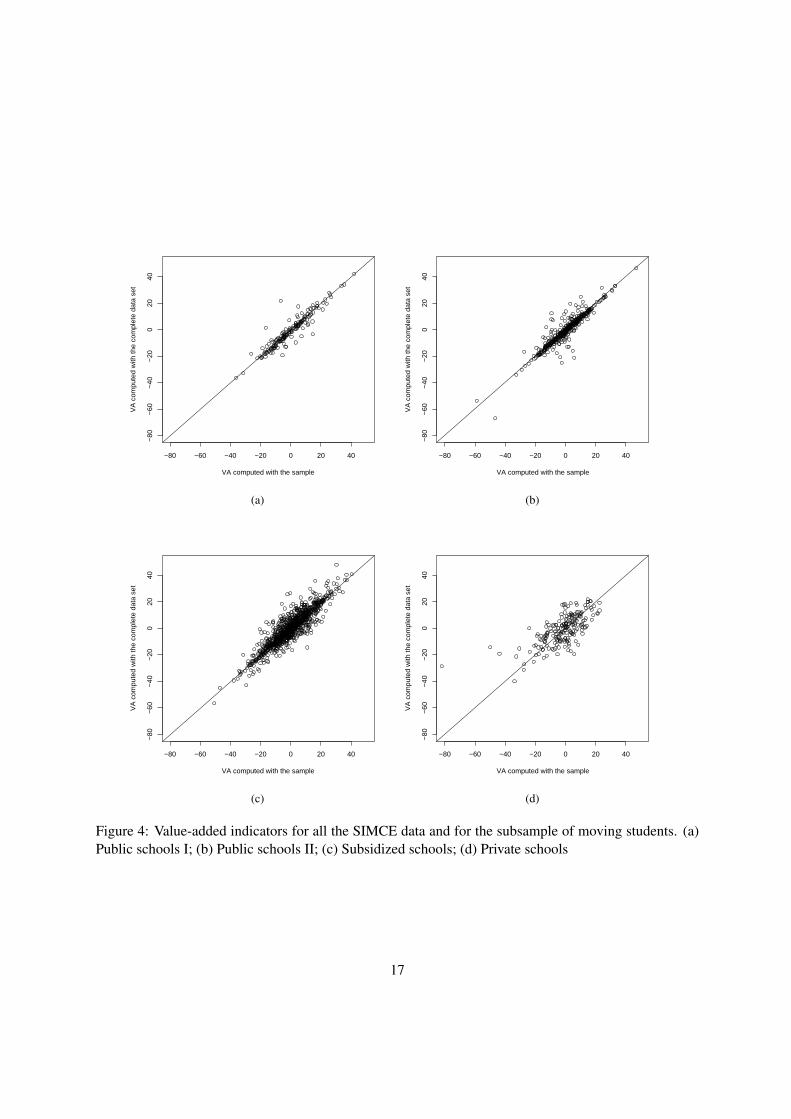
−80 −60 −40 −20 0 20 40
−80
−60
−40
−20
020
40
VA computed with the sample
VA
com
pute
d w
ith th
e co
mpl
ete
data
set
(a)
−80 −60 −40 −20 0 20 40
−80
−60
−40
−20
020
40
VA computed with the sample
VA
com
pute
d w
ith th
e co
mpl
ete
data
set
(b)
−80 −60 −40 −20 0 20 40
−80
−60
−40
−20
020
40
VA computed with the sample
VA
com
pute
d w
ith th
e co
mpl
ete
data
set
(c)
−80 −60 −40 −20 0 20 40
−80
−60
−40
−20
020
40
VA computed with the sample
VA
com
pute
d w
ith th
e co
mpl
ete
data
set
(d)
Figure 4: Value-added indicators for all the SIMCE data and for the subsample of moving students. (a)Public schools I; (b) Public schools II; (c) Subsidized schools; (d) Private schools
17

In the last part of this paper, we consider a new estimation of the value-added that is robust to theendogeneity of mat04ij or avmat04j .
4.4 Value-added under endogeneity
The principal consequence of the endogeneity of the lagged score is that the prediction of the randomeffect in HLM models does no longer represent the value-added. Recall the definition (3) of the value-added in the context of the HLM model (2). If we consider this model without assuming the exogeneityof the covariates, then the value-added under endogeneity is given by
VAj = θj − E(θj | mat04ij , avmat04j ,XXXij) (4)
for all i. This formula shows that the value-added is given by the prediction of the random effect θjcorrected by a term that is vanishing when all covariates are exogenous.
In the following we examine the impact of this correction on SIMCE data. First of all, we need toconstruct a prediction of the random effect and, to this end, to consistently estimate the parameters ofthe endogenous HLM model. This step uses an instrumental variable approach that enables to separatethe variation of θj from the variation of mat04ij . In our context, a variable is called instrumental ifit is independent from the school-specific effect but is correlated to the endogenous variables mat04ijand avmat04j . Among the vast literature on estimation by instrumental variables, we cite the survey byAngrist and Krueger (2001). In Ebbes et al. (2004), instrumental variable techniques are more specifi-cally applied on multilevel models. Estimation by instrumental variables is nowadays included in a lotof softwares, such as Stata (Baum, 2006). In Appendix A below, we fully describe this statistical model,and also give the complete algorithm for computing the value-added under endogeneity.
A delicate question in empirical analysis is of course the choice of instrumental variables. In theSIMCE study, we considered the level of education of the father and the level of education of the motheras instruments. The fact that these two variables are correlated with the score of a student is a confirmedfact that is supported by many statistical studies; for the Chilean case, see, e.g., Sapelli and Vial (2002);Paredes and Paredes (2009); for the american test “TIMMS”, see, e.g., Kyriakides (2006); Thomson(2008); for a general discussion, see Hanushek (2006). Moreover, in the SIMCE data set, the correlationbetween fathed and mat04 is 0.38, and between fathed and avmat04 is 0.55, whereas the correlationbetween mothed and mat04 is 0.39, and between mothed and avmat04 is 0.55. It is also plausibleto assume that they are independent from the school-specific effect, mainly because the parents werenot educated in the school of their children. At this stage, it is also important to note that we havecontrolled for other covariates in the HLM model such as the variable select. This point is importantbecause the selection might be a common factor between parents education and the score of their student.Conditionally on this variables (and on all other covariates), our assumption is thus that parents educationis independent from the school-specific random effect.
We present results of estimation under HLM5 specification, in which mat04ij and avmat04j are con-sidered as endogenous, and fathed and mothed are instrumental variables. Having predicted the randomeffect from this estimation, which we denote by θIV
j , we then compute a regression on θIVj to estimate
the correction term of the value-added in (4). At this stage, we note that several options are possi-ble to compute the correction term. In this paper we specify a linear model for the correction termE(θj | mat04ij , avmat04j ,XXXij). Because XXX ij contains exogenous variables, we do not include those
18
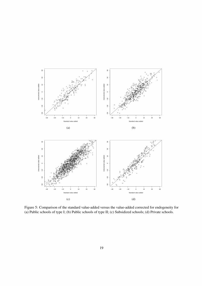
−30 −20 −10 0 10 20 30
−30
−20
−10
010
2030
Standard value added
Inst
rum
enta
l val
ue a
dded
(a)
−30 −20 −10 0 10 20 30
−30
−20
−10
010
2030
Standard value added
Inst
rum
enta
l val
ue a
dded
(b)
−30 −20 −10 0 10 20 30
−30
−20
−10
010
2030
Standard value added
Inst
rum
enta
l val
ue a
dded
(c)
−30 −20 −10 0 10 20 30
−30
−20
−10
010
2030
Standard value added
Inst
rum
enta
l val
ue a
dded
(d)
Figure 5: Comparison of the standard value-added versus the value-added corrected for endogeneity for(a) Public schools of type I; (b) Public schools of type II; (c) Subsidized schools; (d) Private schools.
19

variables in the linear specification. We thefore estimate the conditional expectation by a linear regres-sion of avmat04j on θIV
j with school type fixed effects. The estimated coefficients of the regressionis
θIVj = 46.63 + 5.9δPP − 3.9δII − 4.2δI − 0.17avmat04j + ηj
where δPP , δII , δI are dummy variables for private, type II and type I schools respectively. All estimatedcoefficients have p-value less that 0.01.
Figure 5 shows the value-added obtained from (4) versus the value-added obtained from a standard,exogeneous HLM analysis. The Spearman’s rank correlation between the two calculations of the value-added over the whole sample is 0.9. This quantifies the impact of the correction on the ranking ofschools. This correlation is similar for each schooltype: it is 0.9 (Public type I schools), 0.86 (Publictype II schools), 0.91 (Subsidized schools) and 0.93 (Private schools).
To interpret the change in the calculated value-added it is useful to look at the density of the value-added by type of school. Figure 6(a) superimposes the density of the standard value-added for publicschools (type I, dashed line) and subsidized schools (solid line). The same picture after the correction forendogeneity is displayed in Figure 6(b). The gap that appeared in Figure (a) between the mode of the twotypes of schools is clearly reduced after the correction. The same conclusion is made when comparing thevalue-added of public schools and private schools (Figures (c) and (d)). It is also worth mentionning thattwo modes appear in the value-added of public schools after correction for endogeneity. The emergenceof differentiated public schools according to their effectiveness is an interesting substantive question forfurther research.
5 Conclusion
The main message of the paper is the following. In models of value-added, the lagged test score that isincluded as an explanatory variable is very often endogenous. It is in particular the case when there islittle mobility of students between the test occasions. We have shown the impact of this endogeneity onthe calculation of the value-added from a linear multilevel model, and we have developed a value-addedcalculation that is robust to this endogeneity.
The paper also raised several questions for further research. We would like to conclude by summarizingthree such questions.
1. The value-added under endogeneity is the prediction of the school random effect plus a correctionterm that we have found to be a conditional expectation, see the above equation (4). In this paper,the correction term is considered as linear but of course other choices might be possible here. Astudy of the specification of this correction term would be valuable for the generic calculation ofthe value added under endogeneity.
2. The paper provides a structural definition of the value-added as a difference between two condi-tional expetations, see equation (3). When the multilevel regression is used to model the scoreevolution, it implies that those two conditional expectations are linear. However non linearities ofsome explanatory variables (including the lagged score) is questionable and might be supportedby a nonparametric analysis of the variables in presence. The definition of the value-added givenby equation (3) opens the door for a nonlinear analysis of score evolution.
20

−60 −40 −20 0 20 40 60
0.00
00.
005
0.01
00.
015
0.02
00.
025
0.03
0
(a)
−60 −40 −20 0 20 40 60
0.00
00.
005
0.01
00.
015
0.02
00.
025
(b)
−40 −20 0 20
0.00
00.
005
0.01
00.
015
0.02
00.
025
0.03
0
(c)
−60 −40 −20 0 20 40 60
0.00
00.
005
0.01
00.
015
0.02
00.
025
(d)
Figure 6: Density of the standard value-added (a and c) and density of the value-added corrected forendogeneity (b and d). The dashed, red line is the density for public type I schools. The solid, black lineis the density for subsidized schools (a and b) and private schools (c and d).
21

3. A substantive question appeared in our analysis of the value-added under endogeneity for publicschools in Chile. As we have shown in Figure 6, the value-added of those schools is bimodal,suggesting the existence of two distinct groups of public schools according to their effectiveness.One mode is even larger than the mode we have found for private or subsidized schools. This resultcalls for further investigation and characterization of public schools that belong to one or the othermode.
A Instrumental HLM modelling
For the sake of generality, we denote by Yij the contemporaneous score of student i belonging to schoolj and by Zij the endogenous variables. In our application, Zij contains covariates depending on thelagged score. We also recall the notation XXXij for the vector of exogeneous explanatory covariates and θjfor the school-specific latent effect. By endogeneity, we mean that the covariance between θj and Zij
is not vanishing. To solve the endogeneity issue, we suppose to have a vector of instrumental variables,denoted byWWW ij . The intuition behind instruments is that they are correlated to the endogenous variables,but they are not correlated with θj .
We can specify the normal instrumental HLM model as follows:
(i) (Yij | Zij ,XXXij ,WWW ij , θj) ∼ N(XXXijβ + γZij + θj , σ
2)
(ii) (Zij |XXXij ,WWW ij , θj) ∼ N(XXX ijααα+WWW ijζζζ + δθj , τ
2)
(iii) (θj |XXXij ,WWW ij) ∼ N(0, µ2
).
Condition (iii) implies that E(θj | XXXij ,WWW ij) = 0 and, therefore, (Xij ,W ij) and θj are uncorrelated.In other words, both XXXij and WWW ij are exogenous variables with respect to θj . Condition (i) implies that,conditionally on (Zij ,XXX ij , θj), the contemporaneous score Yij is mutually independent of WWW ij . Thus, if(i) is rewritten as
Yij =XXXijβ + γZij + θj + ϵij , ϵij ∼ N(0, σ2),
then E(ϵij | WWW ij) = 0. This condition, along with cor(WWW ij , θj) = 0, define WWW ij as an instrument. Itcan be shown that the parameters of the instrumental HLM model are identified provided the dimensionof the vector WWW ij is at least equal to the number of endogenous variables. Finally, the distribution of(XXX ij ,WWW ij) is left unspecified as it is typically done for exogenous variables; see Engle et al. (1983),Florens et al. (1990, Chapter 3) and Hendry (1995).
It should be remarked that a classical HLM assumes that (θj | Zij ,XXXij ,WWW ij) ∼ N(0, µ2), instead ofconditions (ii) and (iii) as the instrumental HLM. In particular, E(θj | Zij ,XXXij ,WWW ij) = 0 and, therefore,Zij ,XXXij and WWW ij are uncorrelated with θj . This condition implies that XXXij and WWW ij are uncorrelatedwith θj , but the converse is far from being true.
The value-added indicator is calculated using the following steps:
1. Estimate consistently parameters β and γ by instrumental variable estimation.
2. Predict the random effect and get θj .
22
3. Regress θj on the average of all covariates Z·j and WWW ·j , and store the predictions θj from this
regression.
4. Compute the value-added as θj −θj .
Acknowledgements: We thank Jorge Gonzalez, Daniel Koretz, Michel Mouchart and Sally Thomasfor helpful discussions. This paper was presented at the International Meeting on School Progress andValue-added Models organized by the Measurement Center MIDE UC, May 2010, Santiago, Chile. Thiswork was supported by the “Agence National de le Recherche” under contract ANR-09-JCJC-0124-01and the CORFO INNOVA Grant No. 07CN13IEM-91 Development of standardized tests and of a value-added methodology to assess progress of learning in Mathematics and Language students, second cycleof primary school. The authors are grateful to the SIMCE Office of the Chilean Ministry of Educationfor providing access to the database. All opinions and conclusions expressed in this paper are those ofthe authors and not of the Ministry of Education.
References
Angrist, J. D. and A. B. Krueger (2001). Instrumental variables and the search for identification: Fromsupply and demand to natural experiments. Journal of Economic Perspectives 15, 69–85.
Baum, C. F. (2006). An introduction to modern econometrics using Stata. College Station: Stata press.
Bellei, C. (2005). ¿Ha tenido tenido impacto la reforma educativa chilena? In C. Cox (Ed.), PolıticasEducacionales en el cambio de siglo. La reforma del sistema escolar de Chile. Editorial Universitaria,Santiago de Chile.
Bellei, C., D. Raczynski, G. Munoz, and L. Perez (2004). ¿Quien dijo que no se puede?: EscuelasEfectivas en Contextos de Pobreza. Santiago, Chile: UNICEF.
del Pino, G., J. Gonzlez, J. Manzi, and E. San Martın (2009). Estudio Piloto de Valor Agregado 3oBasico 2006 - 4o Medio 2007. Santiago, Chile: Report for the Ministry of Education of the ChileanGovernment.
del Pino, G., E. San Martın, J. Manzi, and S. Taut (2008). Estudio Piloto de Valor Agregado 8o Basico2004 - 2o Medio 2006. Santiago, Chile: Report for the Ministry of Education of the Chilean Govern-ment.
del Pino, G., E. San Martın, J. Manzi, S. Taut, and J. Gonzalez (2008). Estudio Piloto de Valor Agregado4o Basico 2005 - 5o Basico 2006. Santiago, Chile: Report for the Ministry of Education of the ChileanGovernment.
Ebbes, P., U. Bockenholt, and M. Wedel (2004). Regressor and random-effects dependencies in multi-level models. Statistica Neerlandica 58, 161–178.
Embretson, S. E. and S. P. Reise (2000). Item Response Theory for Psychologists. New Jersey: LawrenceErlbaum Associates, Publishers.
23

Engle, R. E., D. F. Hendry, and J. F. Richard (1983). Exogeneity. Econometrica 51, 277–304.
Eyzaguirre, B. (2004). Claves para la educacion en pobreza. Estudios Publicos 93, 249–277.
Florens, J.-P., M. Mouchart, and J.-M. Rolin (1990). Elements of Bayesian Statistics. New York: MarcelDekker.
Goldstein, H. and D. Spiegelhalter (1996). League Tables and Their Limitations: Statistical Issues inComparison of Institutional Performance. Journal of the Royal Statistical Society, Series A 159, 385–443.
Goldstein, H. and S. Thomas (1996). Using examination results as indicators of school and collegeperformance. Journal of the Royal Statistical Society, Series A 159, 407–442.
Grilli, L. and C. Rampichini (2009). Measurement error in multilevel models with sample cluster means.Working Paper 2009/06, Universita degli Studi di Firenze.
Halaby, C. (2004). Panel models in sociological research: Theory into practice. Annual Review ofSociology 30, 507–544.
Hanushek, E. A. (2006). School resources. In E. A. Hanushek and F. Welch (Eds.), Handbook of theEconomics of Education, Amsterdam, pp. 865–908. Elsevier.
Hendry, D. F. (1995). Dynamics Econometrics. Oxford: Oxford University Press.
Hutchison, D., C. Mifsud, J. Morrison, R. Grech, P. Rudd, and J. Hanson (2005). The Malta primaryliteracy value-added project: a template for value-added in small island states? Research Papers inEducation 20, 303–345.
Kim, J.-S. and E. W. Frees (2006). Omitted variables in multilevel models. Psychometrika 71(4), 659–690.
Kim, J.-S. and E. W. Frees (2007). Multilevel modelling with correlated effects. Psychometrika 72(4),505–533.
Kyriakides, L. (2006). Using international comparative studies to develop the theoretical framework ofeducational effectiveness research: A secondary analysis of TIMSS 1999 data. Educational Researchand Evaluation 12, 513–534.
Lockwood, J. R. and D. F. McCaffrey (2007). Controlling for individual heterogeneity in longitudinalmodels, with applications to student achievement. Electronic Journal of Statistics 1, 223–252.
Marshall, G., I. Huerta, A. M. Alvarado, and J. Ponce (2008). Clasificacion de Escuelas. SubvencionEscolar Preferencial 2008-2009. Santiago, Chile: Report for the Ministry of Education of the ChileanGovernment.
OECD (2007). Science Competencies for Tomorrow’s World. Volumen 1: Analysis. Programme forInternational Student Assessment, Organisation for Economic Co-operation and Development OECD.
24
OECD (2008). Measuring Improvements in Learning Outcomes. Best Practices to Assess the Value-Added of Schools. Organisation for Economic Co-operation and Development OECD.
Paredes, R., C. Dagnino, C. Del Canto, G. Espinosa, F. Lagos, V. Ramırez, E. San Martın, and Y. Stekel(2010). Determinacion de Estandares e Indicadores de Condiciones para el Aprendizaje en Establec-imientos Educacionales. Santiago, Chile: Report for the Ministry of Education of the Chilean Gov-ernment.
Paredes, R. D. and V. Paredes (2009). Chile: academic performance and educational management undera rigid employment regime. CEPAL Review 99, 117–129.
Raudenbush, S. W. (2004). What are value-added models estimating and what does this imply for statis-tical practice? Journal of Educational and Behavioral Statistics 29, 121–129.
Raudenbush, S. W. and J. D. Willms (1995). The estimation of school effects. Journal of Educationaland Behavioral Statistics 20, 307–335.
Sapelli, C. and B. Vial (2002). The Performance of Private and Public Schools in the Chilean VoucherSystem. Cuadernos de Economıa 39, 423–454.
Silverman, B. W. (1986). Density Estimation. London: Chapman and Hall.
SIMCE (2008). Niveles de Logro 4o Bsico para Educacion Matematica. Unidad deCurrıculum y Evaluacin (UCE), Ministerio de Educacion, Gobierno de Chile. Available athttp://www.simce.cl/index.php?id=419.
SIMCE (2009). Resultados Nacionales SIMCE 2008. Unidad de Currıculum y Evaluacin (UCE), Min-isterio de Educacion, Gobierno de Chile. Available at http://www.simce.cl/index.php?id=430.
Spencer, N. H. (2008). Models for value-added investigations of teaching styles data. Journal of DataScience 6, 33–51.
Steele, F., A. Vignoles, and A. Jenkins (2007). The effect of school resources on pupil attainment: amultilevel simultaneous equation modelling approach. Journal of the Royal Statistical Society: SeriesA 170, 801–824.
Tekwe, C. D., R. L. Carter, C. X. Ma, J. Algina, M. E. Lucas, J. Roth, M. Ariet, T. Fisher, and M. B.Resnick (2004). An Empirical Comparison of Statistical Models for Value-Added Assessment ofSchool Performance. Journal of Educational and Behavioral Statistics 29, 11–36.
Thomson, S. (2008). Examining the Evidence from TIMSS: Gender Differences in Year 8 ScienceAchievement in Australia. Studies in Educational Evaluation 34, 73–81.
25