CONTROL SYSTEM DESIGN FOR AN

AUTONOMOUS MOBILE ROBOT

A thesis submitted to the Division of

Graduate Studies and Advanced Research

of the University of Cincinnati

in partial fulfillment of the

requirements for the degree of

MASTER OF SCIENCE

In the Department of Mechanical, Industrial and Nuclear Engineering

of the College of Engineering

2000

by

Sathish K. Shanmugasundaram

B.E (Mechanical Engineering), PSG College of Technology

Coimbatore, India

Thesis Advisor and Committee Chair: Dr. Ernest L. Hall

Abstract

A good control system is an absolute requirement for a mobile robot or, for any system

that has to be automated. This thesis deals mainly with designing an optimal, stable

control system for an autonomous robot. The robot is Bearcat II. Bearcat II is being

developed as an automated guided vehicle to participate in the annual International

Ground Robotics Competition automated vehicles contest.

A closed loop control system called as proportional, integral, and derivate control system

(PID) is used currently on the robot. It uses an elaborate algorithm to manipulate the

parameters. Tuning of the controller is the real tricky part of these types of controllers.

Various tuning methods currently in use are discussed. The difficulties in using these are

also highlighted. The model of the control system is reviewed and the system response

studied. A general model of a motor and load system is also developed.

Based on the model, a new technique using optimization theory is developed. This theory

concentrates on reducing the error between output and input at multiple instants of time.

This is a multi-criteria optimization formulation of the problem. Methods used in the

formulation are discussed. Finally, an optimized set of tuning constants is determined.

The developed method is more logical, scientific and better in terms of minimal mean

square error than previous methods. It also reduces the number of iterations required for

tuning the controller.

Acknowledgements

First, I would like to sincerely thank Dr. Ernest Hall my advisor, for having pointed me to

this direction and, for his enthusiastic and energetic guidance throughout my career at the

University of Cincinnati. He has been a constant source of information and support for

this thesis.

A special word of thanks should go the robotic team members, past and present for

having supported in my work. They have helped me in all possible ways to make this

process smooth. I would also like to add a note of thanks and special appreciation to the

staff of the MINE department for having supported the team and me in all possible ways.

My committee members, Dr. Richard L. Shell and Dr. Ronald L. Huston, should be

thanked for looking through my work and making valid suggestion. Their suggestions

have made this work more focused.

Last but not least, my family should be thanked. They have stood by me and watched my

career evolve for the better. They have also been a source of constant support and

encouragement. I love you all very much.

1

Table of Contents

List of Figures………………………………………………………. 4

1. Introduction………………………………………………………….. 6

1.1 Introduction…………………………………………….. 6

1.2 Motivation and problem statement…………………….. 7

1.3 Objective………………………………………………. 7

1.4 Acknowledgement……………………………………… 7

1.5 Organization…………………………………………… 8

2. Background work and literature search…………………………… 9

2.1 Introduction…………………………………………….. 9

2.2 Linear and non-linear controller design ……………… 13

2.3 Parallel linkage steering for an AGV………………... 14

2.4 Modeling and control of an automated vehicle……… 17

3. Control System theory……………………………………………. 20

3.1 Introduction…………………………………………… 20

3.2 The basic control system……………………………… 21

3.2.1 The control problem…………………… 22

3.2.2 Description of the input and output… 23

3.3 Feedback and feed forward control…………………… 24

3.4 Linear control systems………………………………… 29

2

3.5 Control of non-linear systems………………………… 30

3.6 The design process…………………………………….. 32

4. PID and the Galil DMC1000 controller. …………………………. 38

4.1 Digital control systems……………………………….. 38

4.2 PID controller…………………………………………. 44

4.2.1 Proportional band.……………………………… 46

4.2.2 Integral.………………………………………… 47

4.2.3 Derivative.……………………………………… 48

4.3 Control loop tuning…………………………………… 50

4.4 Galil DMC 1000……………………………………… 55

4.5 Microcomputer section……………………………… 57

4.6 Motor Interface……………………………………… 57

4.7 Communication……………………………………… 58

4.8 General I/O.………………………………………… 58

4.9 Amplifier.…………………………………………… 58

4.10 Encoder…………………………………………… 59

5. Control parameter determination for the current robot……. 61

6. Simulation and optimizing the parameters………..………. 65

6.1 Introduction.………………………………………. 65

6.2 Simulation on SIMULINK.………………………… 65

3

6.3 SIMULINK model…………………………………. 68

6.4 Optimizing the control system……………………… 69

6.5 The lsqnonlin method………………………………. 70

7. Results and summary…………………………………………… 74

8. Recommendations……………………………………………… 75

9. References ...……………………………………………………. 76

10. Appendix………………………………………………………… 83

4

List of figures Page Chapter 2 2.1 Lane following feedback structure…………………………. 7 2.2 Design of experimental automated guided vehicle………… 11 2.3 Control system……………………………………………… 13 2.4 Closed loop system performance……………………………. 14 Chapter 3 3.1 Simplified description of a control system…………………… 17 3.2 Input output for the elevator system…………………………. 19 3.3 A typical feedback control system……………………………. 21 3.4 An antenna azimuth position control system………………… 28 3.5 Functional block diagram of a position control system……… 29

Chapter 4 4.1 An example of a 3-bit quantized signal………………………… 36

4.2 A control system……………………………………………….. 37 4.3 A digital control system controlling a controlling a cont. plant… 38 4.4 PID equations…………………………………………………… 41

5

4.5 A time response plot showing controller action…………………. 43 4.6 Controller frequency response plot………………………………. 45 4.7 A cruise controller………………………………………………….. 48

Chapter 5 5.1 Start-up menu of Galil motion control…………………………….. 57 5.2 Tuning methods menu of the Galil motion control………………. 58 5.3 Step response plot from the Galil servo design kit………………. 59

Chapter 6 6.1 Simulink model of the system………………………………………. 62 6.2 Step response for the system………………………………………. 63 6.3 General motor and load control system…………………………….. 64 6.4 Step response for the general system………………………………. 65 6.5 Error diagram…………………………………………………………… 66

6

Chapter 1

Introduction

1.1 Introduction

Control systems are the very heart of mobile robots. Problems such as coordination of

manipulators, motion planning and coordination of mobile robots require a central

controller. Motion control is one of the technological foundations of automation. Whether

the motion of a product, path of a cutting tool, motion of a robot arm, the control of

motion is a fundamental concern. To be able to control a motion process, the precise

position of objects needs to be measured. Then a feedback comparison of the target and

actual positions is then a natural step in implementing a motion control system. This

comparison generates an error signal that may be used to correct the system. If the error

is small, the system performance is repeatable and accurate. However, the use of

feedback can lead to an unstable system whose output can go to infinity with a small

input signal. This shows the importance of a good control system design. Many feedback

controllers use a proportional-derivative-integral algorithm to manipulate the error signal

and apply a corrective effort to the process.

7

1.2 Motivation and problem statement

The main motivation of this thesis is the mobile robot Bearcat II that we are developing

and continually improving. The robot uses a PID controller (Reference). Though this type

of controller is common it is very hard to tune and attain stable PID parameters. The team

has tried many different methods to tune the controller.

A few of them are iterative trial and error and, brute force. Though these work for most

situations, the stability of the system is lost at certain times. For example using the largest

possible values could make the controller very aggressive and cause amplification of

errors. On the other hand if the tuning it too conservative does not eliminate the errors

and the system appears sluggish. Hence this is a difficult adaptive tuning process.

1.3 Objective

To solve this problem a new technique using optimization theory is proposed in this

thesis. It uses both simulation and optimization. Because it uses an objective criteria

function, minimum mean square error, it is a more scientific and logical approach to the

problem. Although it is not a perfect and final solution, it is a definite step toward

reaching the perfect and one solution for these adaptive controllers.

1.4 Acknowledgement

This thesis is an extension to the work done in this area especially by two previous team

members, Kalyan Kolli and Krishna Mohan Kola. Some of the ideas and topics have been

8

derived from their work and have been worked on and extended. We acknowledge them

for their good and fascinating work.

1.4 Organization

Chapter 2 deals with the introduction and survey of automated guided vehicles. Chapter 3

gives an introduction to control system theory and the various types of control techniques

used. Chapter 4 looks at the PID controller used in the Bearcat II, Galil DMC 1000

controller. It also explains the purpose and meaning of the various parameters in the PID

controller. Chapter 5 details the current tuning procedure for the Bearcat II. The software

used to assist the tuning is described in detail. Chapter 6 models the control system and

brings out the new optimization technique for parameter determination. Finally the results

and recommendations for future work are discussed in Chapter 7. The Appendix shows

the actual Matlab and Simulink code used to obtain the results.

9

Chapter 2

Background work and literature search 2.1 Introduction

Automated guided vehicle systems (AGVS) are commonly used for transporting material

within a manufacturing, warehousing, or distribution system. These systems provide for

asynchronous movement of material through the system and are used in a wide variety of

applications. They offer many advantages relative to other types of material handling

systems, including reliable, automatic operation, flexibility to changes in the material

handling requirements, improved positioning accuracy, reduced handling damage, easily

expandable layout and system capacity, and automated interfaces with other systems

(Miller, 1987)(References should be numbered and listed in the Reference List in order

they are encountered in the text).

2.1.1 Classification of AGV’s – Following are the ways AGV’s are classified

1. Guide path determination

10

1. Static path

1. Unidirectional

2. Bi-directional

2. Dynamic path

2. Vehicle capacity

1. Single unit load

2. Multiple loads

3. Vehicle addressing mechanism

1. Direct address

2. Indirect address

Most AGVs have a specification of maximum speed about 1 m/sec (3.28 ft/sec, 2.24

mph) although, in practice, they are usually operated at half that speed. In a fully

automated manufacturing environment, there should be few personnel in the area;

therefore, the AGV should be able to run at full speed. As the speed of the AGV

increases, so does the difficulty in designing stable and smooth tracking controls.

11

Consequently, it becomes important to understand the dynamic effects of various design

parameters on the steering action of the AGV.

Work has been done in the past to analyze various aspects of steering control in different

situations for automobile steering or mobile robots. Some deals with the kinematics and

dynamics involved (Tagawa et al [11]; and others have dealt with the controller designs

for a linear or non-linear control (Hattori et al [19]).

Ozguner, et al [3] described an analytical study of vehicle steering control. They

considered the design and stability analysis of a steering controller. The objective of the

controller was to steer a ground vehicle along a reference line located in the middle of the

lane. An arbitrary look-ahead point was located on the local longitudinal axis of the

vehicle. The displacement between the look-ahead point and the reference point was

called the look-ahead offset. During perfect lane tracking, the ratio of the steering angle

to the look-ahead offset was independent of the curve radius under reasonable

approximations. That ratio was computed in terms of the vehicle speed and various

vehicle parameters. Then, a constant controller was designed to achieve that ratio at

steady state. The controller was updated as a function of the vehicle speed. The only

information processed by the controller was the look-ahead offset, which was measured

using a radar-based or vision-based sensor. Using Routh-Hurwitz analysis, it was

analytically proven that the closed loop system is stable. Given any range of longitudinal

12

speeds, there exists a sufficiently large look-ahead distance ensuring the closed loop

closed-loop stability for all speeds in that speed range.

The look-ahead information was a set of geometrical information, including road

feedback topology ahead of the vehicle center of gravity and the vehicle’s orientation and

position relative to the topology. In this paper the objective was to develop a new control

law for automatic steering based on specific look-ahead information.

The paper considered the vehicle model and discussed the control design and the stability

analysis of the controller. A simulation example was presented.

The mathematical block diagram of the proposed model was a shown in the Figure 2.1

below.

Figure 2.1 Lane following feedback structure (Ozguner, et al. [3])

The authors conclude that the controller was successfully tested at the Transportation

Research Center, Marysville, OH.

L o o k - a h e a d o f f s e t

S e n s o r

C o n s t a n tC o n t r o l l e r S t e e r a n g l e

C o m m a n d

V e h i c l e d y n a m i c s &V e h i c l e - r o a d i n t e r a c t i o n

L o n g i t u d i n a l S p e e d

13

2.2 Linear and non-linear controller design for robust automatic steering

Ackerman, et al4 proposed a “linear and non-linear controller design for robust steering.”

The research work presented by them concentrated on the automatic steering of vehicles,

which they described as part of an integrated system of integrated highway system of the

future. The primary task of an automated steering is to track a reference path, where the

displacement sensor measures the displacement from the guide path. The reference may

consist of a magnetic field of an electrically supplied wire or permanent magnets in the

road. The sensor is mounted in the center of the front end of the vehicle. The controller

output acts on the front wheel steering angle.

The design of an automatic steering system is a robustness problem in view of the large

variations in velocity and mass of the vehicle and contact between tire and road surface.

In the proposed research the authors model the data and specifications for a city bus. A

comparison was then made between linear and non-linear controller concepts.

For non-linear control it was investigated that the track accuracy was improved by

additional feedback of the yaw rate, which could be measured by a gyro. Therefore the

automatic control problem became much less dependent on the uncertain operating

conditions of velocity, mass, and road-tire contact. The study showed a significant

reduction in the displacement from the guideline for all maneuvers and operating

14

conditions. In their study, the design method used the parameter space approach, which

was further exploited to explore extreme design directions. The resulting controller with

fixed gains achieved good performance for a wide range of uncertainty in the operating

conditions.

Additionally, in their research a non-linear controller structure was designed in an effort

to further improve the performance of the automatic steering system. The non-linear

controller was based on sliding mode control and included dynamic adaptation to

changing operating conditions via an estimator-like observer. The advantages and

drawbacks of the two approaches were contrasted in simulation studies. Finally,

controller parameters of both the linear and non-linear controller were tuned

automatically by optimizing a vector performance for typical maneuvers.

2.3 Parallel Linkage Steering for an Automated Guided Vehicle.

Sung, et al [5] have considered in their work a parallel linkage steering for an automated

guided vehicle. The paper described the computer-aided design of suitable control

strategies for parallel linkage steering of an experimental automated guided vehicle. The

microprocessor-based steering control system was modeled, and stability characteristics,

15

using proportional control, were investigated via describing functions. Although the

approximation is coarse, the analysis indicates the upper bound for gain and suggests

derivative action for improved control. For better accuracy, a flexible and fast simulation

program was developed that enabled an efficient search for “optimal” control laws for

operation of the vehicle under the constant speed mode and the slow-down mode. Time-

independent control laws were investigated, and the solutions found gave tolerable

tracking over 90-deg arcs of 0.5-m radius. The simulation results were shown in which

the time dependent control laws were proved to be essential for improved, nonoscillatory

tracking. The experimental AGV has a differential gear drive and parallel linkage steering as

shown in Figure 2.4.

Figure 2.2 Design of experimental automated guided vehicle (Sung, et al. [5] )

Six infrared sensors [light emitting diodes (LEDs)] were used on the forward and reverse

guidance systems. Because of the designed configuration of the wheel positions, the

AGV was symmetrical in the forward and reverse directions, which simplified bi-

16

directional control. A DC servomotor was used for the drive; a stepper actuated the

steering wheels. The steering loop was closed by a microprocessor-based-controller that

computed the steering control signal to the stepper motor based on the derivation of the

AGV from the track. The track contained reflective tape, and the derivation was

measured by discrete number of LEDs “out of track”. This coarse sensing method was

selected over more sophisticated continuous sensors for cost reasons but at the expense of

the anticipated poorer tracking response.

The critical parameters affecting the steering action of the AGV were identified as

follows:

1. Method of sensing the deviation from the guide path

2. Geometrical configuration of the AGV’s wheels

3. Speed of the AGV and drive dynamics in case of variable speed operation

4. Steering angle as a function of the deviation, i.e., the control strategy or control

law.

Parameters 1 and 2 above pertained to the AGV firmware, whereas items 3 and 4 are

required to be designed on the basis of firmware. It was desirable to operate the AGV at

its maximum speed (constant) all the time but as was seen in the research study that was

not possible when the AGV was negotiating a curve. Thus, the computer-aided design

focused on finding:

17

1. The maximum speed possible in the constant speed mode of operation and the

associated optimal control law

2. A suitable slow-down mode of operation for the AGV at 1m/sec and the

associated optimal control law

2.4 Modeling and Control of an Automated vehicle

Will and Zak, [6] present a vehicle model that includes the vehicle dynamics and vehicle

dynamic model. The model developed was then used for conducting steering analysis of

an automated vehicle. They tested the developed model on a step lane change maneuver

and proposed a model-reference-based controller for the remote control of a vehicle.

Stability analysis of the closed-loop system using the Lyapunov approach was included.

One of the main objectives of their research was to develop a vehicle model that could be

used to predict the dynamics for steering and braking maneuvers. They proposed a model

that is a spring mass system acting under the influence of tire forces developed by three

driver inputs. Those inputs were the front and rear wheel angles and the brake force.

Another objective of their study was to develop design control strategies for

automatically guided vehicles. They proposed a model-reference tracking controller

design. Figure 2.6 shows the model-reference control system block diagram.

18

Figure 2.3 Model-reference control system block diagram with input scaling (Will and Zak [6] )

Figure 2.4. Not Closed-loop system performance with model-reference tracking

controller (Will and Zak [6] )

19

Figure 2.6 above shows the responses of the truth model to the same input signal. The

truth model was incapable of tracking the desired path when using an open loop control.

To improve the tracking performance, they proposed a closed-loop tracking controller.

The proposed model-reference-based controller required the availability of state

variables. They proposed to use combined controller state estimator compensators that

require only the input and output signals in their implementations. The model was also

discontinuous in the state, which resulted in high activity, referred to as chattering.

Chattering could be reduced in a continuous version of the controller proposed. The

continuous controller was obtained by introducing a so-called boundary layer that

smoothed out the discontinuous controller. However, instead of asymptotic stability, only

a uniform ultimate bounded ness can be guaranteed.

20

Chapter 3 Control System Theory 3.1 Introduction

This chapter presents an introduction to basic control theory and the Galil motion

controller. Control systems are an integral part of modern society. Control systems find

widespread application in the steering of missiles, planes, spacecraft and ships at sea.

With control systems we can move large equipment with a precision that would

otherwise be impossible. We can point large antennas toward the farthest reaches of the

universe to pick up faint radio signals. Moving the antennas so precisely by hand would

be impossible. The home is not without its own control systems. In a videodisc or

compact disc machine, microscopic pits representing the information are cut into a disc

by a laser during the recording process. During playback, a reflected laser beam, focused

on the pits, changes intensity. The changes in light intensity are then converted into an

electrical signal and processes as sound or picture. A control system keeps the laser beam

positioned on the pits, which are cut as concentric circles. A home heating system is a

simple control system consisting of a thermostat or bimetallic material that expands or

contracts with changing temperature. This expansion or contraction moves a vial of

21

mercury that acts as a switch, turning the heater on and off. The amount of expansion or

contraction required to move the mercury switch is determined by the temperature

setting.

3.2 The basic control system

A control system consists of subsystems and processes (or plants) assembled for the

purposes of controlling the output of processes. For example, a furnace is a process that

produces heat as a result of the flow of fuel. This process, assembled with subsystems

called fuel valves and fuel-valve actuators, regulates the temperature of the room by

controlling the heat output from the furnace. Other subsystems, such as thermostats,

which act as sensors, measure the room temperature. In the simplest form, a control

system provides an output response for a given input stimulus as shown in block diagram

form in Figure 3.1.

Figure 3.1 Simplified description of a control system

(Nise, Norman [29])

Control system

Input; stimulus

Desired response

Output; response

Actual response

22

3.2.1 The control problem

A generic closed-loop system consists of :

• input; reference input gives the desired output (usually called a setpoint)

• controller

• plant, a system to be controlled

• measurement device; this allows the current state of the system to be assessed and

generation of an appropriate error signal

• output; the controlled output actually generated by the closed loop system

• reward function; in reinforcement problems, we do not know what the set points are;

instead we get evaluative feedback about how effective our control law is.

There may also be a

• Plant model; having a sufficiently accurate model helps us how to build an optimal

controller.

In general, the plant will be a dynamical system, that is, a system describable by a set of

differential (or difference) equations. The distinction between continuous and discrete

dynamical systems can be significant; in the reinforcement literature, several important

results have been found for the control of discrete systems that do not apply in the

continuous case. First, the difference between feedback and feed forward control needs to

emphasized.

23

3.2.2 Description of the Input and output

The input represents a desired response; the output is the actual response. For example,

when the fourth-floor button of an elevator is pushed on the ground floor, the elevator

rises to the fourth floor with a speed and floor-leveling accuracy designed for passenger

comfort. Figure 3.2 shows the input and output for the elevator system.

Figure 3.2 Input output for the elevator system (Nise, Norman [29])

The push of the fourth floor button is the input and is represented by a step command.

The input represents what the desired output should be after the elevator has stopped; the

elevator itself follows the displacement described by the curve marked elevator response.

Two factors make the output different from the input. The first factor is the instantaneous

change of the input against the gradual change of the output. Figure 3.2 shows that the

physical entities cannot change their state instantaneously. The state changes through a

path that is related to the physical device and the way it acquires or dissipates energy.

This is called the transient response of the system.

24

After the transient response, the physical system approaches its steady-state response,

which is its approximation to the commanded or desired response. The accuracy of the

elevator’s final leveling with the floor is a second factor that could make the output

different from the input. This difference is called the steady-state error.

3.3 Feedback and feed forward control

A feedback controller is designed to generate an output that causes some corrective effort

to be applied to a process so as to drive a measurable process variable towards a desired

value known as the set point. The controller uses an actuator to affect the process and a

sensor to measure the results. Figure 3.1 shows a typical feedback control system with

blocks representing the dynamic elements of the system and arrows representing the flow

of information, generally in the form of electrical signals. Feedback control is an error-

driven strategy; corrections are made on the basis of a difference between the system's

current state, and the desired state. In the simplest case of a linear feedback control, the

corrections are proportion to the magnitude of the difference, or error. This may not work

very well for nonlinear plants, so it is common to multiply these control inputs by a gain

matrix. The desired state acts as an attractor, and the system behaves as a simple spring.

25

Figure 3.3 Most feedback controllers for continuous processes use the proportional-

derivative-integral (PID) algorithm to manipulate the process variable by applying a

corrective effort to the process. (VanDoren Vance J [58]).

Springs are notorious for exhibiting oscillations, so it is common to include some

damping terms. e.g.

r(t) = Kp( x d(t) – x (t)) + Kv (d x(t)/dt); (3.1)

where r(t) is the control input, x (t) the state of the system, x d(t) the target state, Kp the

proportional constant or the damping coefficient, Kv the derivative constant or spring

constant in this case and dx(t)/dt the rate of change of the state of the system.

The damping coefficient, Kp, can be set to give critical damping (a state in which there is

just the right amount of damping to bring the system to the desired output level). Note

that this is a completely model-free approach; the complex dynamical interactions of the

system are considered as errors to be eliminated by feedback. As it stands, Equation (3.1)

is not quite right; constant disturbances like gravity will leave a steady state offset in

26

position. We can never get rid of this (unless we have an infinite value of Kp, so we need

an extra integrative term:

r(t) = Kp( x d(t) – x (t)) + Kv (d x(t)/dt) + KI ! ( x d(t) – x (t)) dt (3.2)

where KI is the integral constant. So now there are three terms in the controller, it is seen

that feedback loops like this are described as a three-term controller, or a proportional,

integrative, derivative (PID) controller.

Virtually all feedback controllers determine their output by observing the error between

the set point and a measurement of the process variable. Errors occur when an operator

changes the set point intentionally or when a process load changes the process variable

accidentally. Feedback control is, by definition, an error-driven process, so there need to

be errors for it to be doing anything. This means that it is very likely that there will be a

path that lags continuously behind the desired path. Also, feedback systems usually take a

finite amount of time to respond to errors, so perturbing oscillations above a certain

frequency will not by corrected. Finally, it should be noted that feedback control might

not be limited to the position of the system; and that feedback control can be defined at

any level. Thus, it is perfectly possible to process feedback error signals at a task level, as

long as we can find a reliable way of decreasing the error.

27

Feed forward (model-based, indirect) control takes an alternative approach; a model of

the dynamics of the system is built, and the inverse dynamics are solved for input torque.

This method has the potential for very accurate control, but depends critically, on the

integrity of the model. If we denote the plant dynamics by x(t) = R(r(t), x(0)) then

r(t) = R-1( xd(t)) (3.3)

This is the inverse dynamics of the plant; given the desired state of the system, this tells

us the control inputs required to achieve that state (assuming such control inputs actually

exists). If, however, we only have a model of the plant, say R^, then the path of the

system will be described by then,

θ(t) = R(R^-1( xd(t))) (3.4)

There could be several reasons for feed forward control to be unsatisfactory:

• It may be impossible to get a sufficiently accurate model of the system, and

the deviation of the produced path from the target may be a rapidly increasingly

28

function of time (due to non-linearities or non- stationarities in the dynamics of the

system).

• Even assuming that our model it perfectly accurate, we may have an error in

the measurement of the initial state of the system, i.e. at t = t0.

• Any external objects that cause the system to deviate from its path will not be

corrected; simply brushing against a surface may introduce errors that cannot be

eliminated.

• It would seem unlikely that the control system is capable of computing

inverse dynamics fast enough, even given a perfect model. This may not be a

problem for dedicated hardware controlling robot arms, but if were concerns about

biological plausibility, then a system using purely feed forward control appears

unrealistic.

It can be useful to think of control problems in a dynamical systems context. If we

consider the plant and the controller as one system, then the control problem can be

construed as placing demands on the dynamics of this combined system. In stable

control, we require that the set point of the plant be a fixed point of the system. We would

also usually require this attractor to be stable: small perturbations from the goal state

should cause the system to converge back to the attractor. We may also be concerned

with the flow field surrounding the fixed point, particularly if we want the system to

collapse onto the goal state as quickly as possible, but without overshooting. The

29

reference model mentioned above is a description of the desired behavior of the

combined system. For example, in designing the control system of an aircraft, we don't

have any desired states, but we will have some idea about how we wish the combined

system to handle.

Most control architectures can be categorized as direct or indirect. Indirect control makes

use of a model of the plant in designing the controller; direct control tries to optimize the

outputs of the plant directly. In the case of indirect control, a further distinction can be

made between on-line and off-line optimization. Off-line optimization allows us to learn

a plant model by observing the plant’s behavior under different conditions (system

identification), and subsequently uses that model to design a controller. In on-line

optimization, the plant has to be controlled all the time, while the plant model is being

learned. This is obviously a much more difficult problem, as the combined system is now

time-variant.

3.4 Linear control systems

Most physical systems have non-linear elements, but in some circumstances it may be

possible to treat them as linear. Then the edifice of linear mathematics, which is very

highly developed, can be employed to yield solutions. If a system only operates over a

small range of input values, then the non-linearities can often be effectively approximated

by linear functions. This may be referred to as operation about some reference point or

30

nominal trajectory; if the non-linear equations are known, then the linearized form of

these equations are often called small perturbation equations. If the non-linearities are

severe enough to render the linearization approach invalid, then there is no general theory

of non-linear control available at present only specific methods. Methods for control in

such circumstances, based on artificial neural and fuzzy logic can be found in various

research works. The methods for control of linear, time-invariant systems are very well

known. The only difficulty is that it requires a moderate amount of linear algebra, which

can at first be intimidating for the uninitiated and often a large amount of computation

that can be intimidating for the fastest computers.

3.5 Control of non-linear systems

Non-linear systems are much more difficult to control than linear systems, mainly

because the system equations are not necessarily solvable. Remembering that solving a

set of differential equations means writing down a closed-form equation describing the

behavior of the system under a whole variety of boundary conditions. Linear, time

invariant (LTI) control is concerned with systems whose behavior we can completely

specify; this means that the addition of carefully designed feedback produces a system

that we know will behave in the desired way. When we can't solve a set of differential

equations analytically, we don't know how the system will behave under a set of

boundary conditions, so they need to treated on a case by case basis.

31

Obviously, controlling such a system is going to be difficult, as we can make no claims

about the response of the system to a control input. Except for a few special cases, we

will not be able to guarantee that the combined system will even be stable, let alone

optimal. These two issues, stability and convergence, are much more difficult in the

nonlinear case. Linear systems theory is extremely well developed, and it is often the case

that convergence and stability for an adaptive controller can be proven. If we're trying to

control, for example, a power plant, it may be that the consequences of the system

becoming unstable are disastrous. This is why control engineers are so concerned about

being able to prove stability, and it's also why they try to linearise systems that are

actually nonlinear. Of course, the other side to this coin is the control problem in biology

where the systems are inherently nonlinear. If we're interested in understanding how

biological control systems work, it seems natural to borrow concepts from engineering.

However, this can lead to us viewing these problems from a rather strange perspective.

Biological systems routinely control highly nonlinear plants, for example, flapping wing

systems, which just could not be controlled with current engineering technology. How

can this be?

The point about biological control systems is that they tend to be rather small, so it seems

implausible that they could possibly model the dynamics of a set of four or six flexible

flapping wings. An optimization method such as evolution has no reason to be concerned

with controllers that are provably stable; it's much more likely to go for the 'quick hack'

32

approach, and let all the unsuccessful designs die. This means that it may be very difficult

to get the data on biological control into some kind of unified framework. Control theory

certainly gives us a way of understanding the nature of biological control problems, but

understanding how the controllers actually work might mean a reinterpretation of control

theory concepts.

3.6 The design process

The design of a control system involves a step-by-step but iterative process. The

following section example of an antenna azimuth position control system is presented.

The azimuth angle output of the antenna, θo (t), follows the input angle of the

potentiometer, θi (t). Figure 3.3 shows the diagram of the system and Figure 3.4 shows

the functional block diagram of the system. The functions are shown above the blocks,

and the required hardware is indicated inside the blocks.

Figure 3.4 An antenna azimuth position control system (Nise, Norman [29] )

33

Figure 3.5 Functional Block Diagram of a position control system (Nise, Norman

[29])

Step 1 : Transform the requirements into a physical system

Antenna example: To design a control system for the position control of the azimuth of

the antenna.

Requirements: To position the antenna from a remote location and describe features such

as weight, and the physical dimensions.

Using these requirements the desired transient response and steady state accuracy are

determined.

34

Step 2: Draw a functional block diagram

Involves the translation of the qualitative description of the system into a functional block

diagram that describes the component parts of the system and shows their

interconnections.

In the antenna example: The bBlock diagram indicates functions as input transducer, the

controller, and relevant descriptions of the amplifiers and the motors.

Step 3: Create the schematic

Process of converting the physical system into a schematic diagram.Relevant

approximations of the system should be made and neglect certain phenomena or else

making it difficult to extract information for the mathematical model.

After a single loop of design involving the analysis and interpretation of the system,

decisions have to be made as to whether or not reasonable approximations were made.

If the designer feels that the system was not described fully, additional parameters are

built into the design schematic.

35

Example: Potentiometers made like neglecting the friction or inertia, although these

mechanical characteristics yield a dynamic response rather than an instantaneous

response.

Implications of the assumptions are that the mechanical effects are neglected and the

voltage across the potentiometer changes instantaneously as the potentiometer shaft turns.

Differential and power amplification: Assuming that the dynamics of the amplifier are

rapid compared to the response time of the motors, hence we model it as pure gain K.

Dc motor: The output speed of the motor is proportional to the voltage applied to the

motor’s armature. Armature consists of both the inductive and resistive effects and we

assume that the inductance is negligible for the DC motor.

Load: The load consists of rotating mass and bearing friction. Hence the model consists

of inertia and viscous damping whose resistive torque increases with speed like the

automobile’s shock absorber or the screen door damper.

Step 4 : Develop a mathematical model (block diagram)

From the schematic, the physical laws such as the Kirchhoff’s laws and Newton’s laws

are used with modifying assumptions.

Kirchoff’s voltage law: The sum of voltages around a closed path equals zero.

Kirchoff’s current law: The sum of electric currents flowing from a node equals zero.

36

Newton’s laws: The sum of forces on a body equals zero, the sum of moments on a body

equals zero.

These laws lead to mathematical models that describe the relationship between input and

output of a dynamic system.

Model 1 : One such model is also a linear time invariant differential equation.

Model 2: Transfer function is another way of modeling a system. This is obtained

from linear time invariant differential equation using what is called the Lap lace

transform.

Lap lace transform can be used for linear systems, but yields more intuitive

information than the differential equations.

Ability to change system parameters and rapidly sense the effect of these changes

on the system’s response.

Model 3: State space methods: Advantage of modeling a system in state space is

that they can be used for systems that cannot be described by differential

equations.

These methods are also used to model systems for simulation the digital

computer.

This representation turns an n-th order differential equation into n simultaneous

first-order differential equations.

37

Step 5: Reduce the block diagram.

Subsystem models are interconnected to form a block diagram of a larger system where

each block has a mathematical description. The step involves the reduction of a large

number of subsystems into a large system single block, with a mathematical description

that represents the system from its input to its output.

Step 6: Analyze and design

Analyze the system to see if the response specifications and performance requirements

can be met by simple adjustments of the system parameters. If the specifications are not

yet met the designer then designs additional hardware in order to affect a desired

performance.

Test inputs are signals that are used analytically and during testing to verify the design.

Some of the standard input signals are impulses, steps, ramps, parabolas, and sinusoids.

These steps were followed in the following analysis and synthesis described in the next

chapter.

38

Chapter 4

The Galil DMC 1000 Controller 4.1 Digital control systems

The rapid development of digital technology has radically changed the boundaries of

practical control system design options. It is now routinely feasible to employ very

complicated, high-order digital controllers and to carry out the extensive calculations

required for their design. These advantages in implementation and design capability can

be achieved at low cost because of the widespread availability of inexpensive, powerful

digital computers and related devices.

A digital control system uses digital hardware, usually in the form of a programmed

digital computer, as the heart of the controller. In contrast, the controller, in an analog

control system is composed of analog hardware, typically analog electronic, mechanical,

electro-mechanical, and hydraulic devices. Digital controllers normally have analog

elements at their periphery to interface with the plant; it is the internal workings of the

controller that distinguish digital from analog control.

39

Digital control systems offer many advantages over their analog counterparts. Among

these advantages are the following:

1. Low susceptibility to environment conditions, such as temperature, humidity,

and component aging.

2. The cost reduction and interference rejection associated with digital signal

transmission.

3. Zero “drift” of parameters.

4. High potential reliability.

5. The ability to perform highly complex tasks at low cost.

6. The potential flexibility of easily making changes in software.

7. Relatively simple interfaces with other digital systems, such as those for

accounting, forecasting, and data collection.

Among the disadvantages are:

1. The introduction of errors (or noise) due to the finite precision of digital

computations and the abrupt changes due to the discrete time nature of digital

control.

2. The need for more sophisticated engineering in order to take advantage of

higher-performance control algorithms.

3. Greater limitations on speed of operation.

4. Greater potential for catastrophic failure.

40

The signals used in the description of control systems are classified as continuous-time or

discrete-time. Continuous-time signals are functions of continuous variable, whereas

discrete-time signals are defined only for discrete values of the variable, usually with

evenly spaced time steps. Discrete-time signals and their manipulators are inherently well

suited to digital computation and are used in describing the digital portions of a control

system. Most often, continuous-time signals are involved in describing the plant and the

interfaces between a controller and the plant it controls. Signals are further classified as

being of continuous amplitude or discrete amplitude. Discrete-amplitude (or quantized )

signals can attain only discrete values, usually evenly spaced. The digital values are also

quantized in amplitude signal shown in Figure 4.1, represented by a 3-bit binary code at

evenly spaced time instants.

Figure 4.1 An example of a 3-bit quantized signal

(Santina, Stubberud, Hostetter [36])

In general, an n-bit binary code can represent only 2n different values. Because of the

complexity of dealing with quantized signals, digital control system design proceeds as if

41

computer-generated signals were not of discrete amplitude. If necessary, further analysis

is then done to determine if a proposed level of quantization error is acceptable.

A general control system diagram with a controller is show in Figure 4.2

Figure 4.2 A control system ( Santina, Stubberud, Hostetter [36] )

The plant is affected by input signals, some of which (the control inputs) are accessible to

the controller, and some of which (the disturbance inputs) are not. Some of the plant

signals (the tracking outputs) are to be controlled, and some of the plant signals (the

measurement outputs) are available to the controller. A controller generates control inputs

to the plant with the objective of having the tracking outputs closely approximate the

reference inputs.

As described earlier, the systems and system components are classified by the nature of

their mathematical model and termed continuous time or discrete time, according to the

type of signals they involve. They are classified as linear if signal components in them

can be superimposed. Any linear combination of signal components applied to input

produces the same linear combination of corresponding output components; otherwise the

system is non-linear. A continuous-time system or component is time invariant if its

properties do not change with time. Any time shift of the input produces an equal time

42

shift of every corresponding signal. If a continuous-time system is not time-invariant,

then it is time varying. On the other hand, if the properties of a discrete-time system do

not change with step, then it is called step-invariant [26]. And, if the discrete-time system

is not step-invariant, then it is step varying.

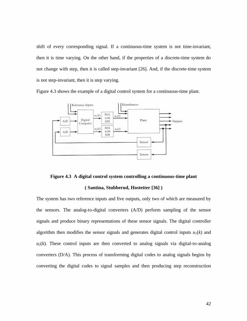
Figure 4.3 shows the example of a digital control system for a continuous-time plant.

Figure 4.3 A digital control system controlling a continuous-time plant

( Santina, Stubberud, Hostetter [36] )

The system has two reference inputs and five outputs, only two of which are measured by

the sensors. The analog-to-digital converters (A/D) perform sampling of the sensor

signals and produce binary representations of these sensor signals. The digital controller

algorithm then modifies the sensor signals and generates digital control inputs u1(k) and

u2(k). These control inputs are then converted to analog signals via digital-to-analog

converters (D/A). This process of transforming digital codes to analog signals begins by

converting the digital codes to signal samples and then producing step reconstruction

43

from the signal samples by transforming the binary coded digital inputs to voltages.

These voltages are held constant for a sampling period T until the next samples are

available. The process of holding each sample to perform step reconstruction is termed

sample and hold.

The system also usually consists of a real-time clock that synchronizes the actions of the

A/D and D/A and the shift registers. The analog signals inputs u1(k) and u2(k) are applied

to the plant actuators or control elements to control the plant’s behavior.

There are many variations on this theme, including situations in which the sampling

period is not fixed, in which the A/D and D/A are not synchronized, in which the system

has many controllers with different sampling periods, and in which sensor produce digital

signals and the actuator accepts digital commands.

Two important classes of control systems are the regulator and the tracking system (or

servo system). In the former, the objective is to bring the system-tracking outputs near

zero in an acceptable manner, often in the face of disturbances. For example, a regulator

might be used to keep a motor-driven satellite dish antenna on a moving vehicle

accurately pointed in a fixed direction, even when the antenna base is moving and

vibrating and the antenna itself is buffeted by winds. In a tracking system, the objective is

for system outputs to track, as nearly as possible, an equal number of reference input

44

signals. Regulation is a special case of tracking, in which the desired system-tracking

output is zero.

4.2 PID controller

PID controllers are designed to eliminate the need for continuous operator attention.

Cruise control in a car and a house thermostat are common examples of how controllers

are used to automatically adjust some variable to hold the measurement (or process

variable) at the set point. A PID controller performs much the same function as a

thermostat but with a more elaborate algorithm for determining its output. It looks at the

current value of the error, the integral of the error over a recent time interval, and the

current derivative of the error signal to determine not only how much of a correction to

apply, but for how long. Those three quantities are each multiplied by a tuning constant

and added together to produce the current controller output CO(t) as shown in Figure

4.4. In this equation, P is the proportional tuning constant, I is the integral tuning

constant, D is the derivative tuning constant, and the error e(t) is the difference between

the set point P(t) and the process variable PV(t) at time t. If the current error is large or

the error has been sustained for some time or the error is changing rapidly, the controller

will attempt to make a large correction by generating a large output. Conversely, if the

process variable has matched the set point for some time, the controller will leave well

enough alone. The set point is where one would like the measurement to be.

45

Figure 4.4 Equations [1] and [6]--both forms of the PID algorithm

generate an output CO(t) according to recent values of the sepoint

SP(t), the process variable PV(t), and the error between them

e(t)=SP(t) - PV(t). (VanDoren Vance J [58])

Error is defined as the difference between the set point and measurement values.

E = S – M (4.1)

Where, E is the error, S is the set point and M is the measurement value.

The variable being adjusted is called the manipulated variable that usually is equal to the

output of the controller. The output of PID controllers will change in response to a

change in measurement or set point. Manufacturers of PID controllers use different

names to identify the three modes. These equations show the relationships:

P Proportional band = 100/gain

I Integral = 1/reset (time units)

46

D Derivative = rate = pre-act (1/units of time)

Where gain is the value of the amplification factor in the control loop, reset is the time

taken for the controller to bring the output to the desired output state and the rate or pre-

act is the actual rate of change of the system stability to achieve the desired state.

Depending on the manufacturer, integral or reset action is set in either time/repeat or

repeat/time. One is simply, the reciprocal of the other. Note that manufacturers are not

consistent and often use reset in units of time/repeat or integral in units of repeats/time.

Derivative and rate are the same.

4.2.1 Proportional

With proportional band, the controller output is proportional to the error or a change in

measurement (depending on the controller).

O = E*100/P (4.2)

Where O is the output of the controller. With a proportional controller, offset (deviation

from set-point) is present. Increasing the controller gain will make the loop become

unstable. Integral action was included in controllers to eliminate this offset.

47

4.2.2 Integral

With integral action, the controller output is proportional to the amount of time the error

is present. Integral action eliminates offset.

Notice that the offset (deviation from set-point) in the time response plots is now gone.

Integral action has eliminated the offset. The response is somewhat oscillatory and can be

stabilized some by adding derivative action.

Figure 4.5: A Time Response plot showing controller action

(Graphic courtesy of ExperTune Inc. Loop Simulator (Expertune Inc [59])

)3.4())((1

∫= dtteI

O

48

Integral action gives the controller a large gain at low frequencies that results in

eliminating offset and "beating down" load disturbances.

4.2.3 Derivative

With derivative action, the controller output is proportional to the rate of change of the

measurement or error. The controller output is calculated by the rate of change of the

measurement with time.

O = D (dm/dt) (4.4)

Where m is the measurement at time t.

Derivative action can compensate for a changing measurement. Thus, derivative takes

action to inhibit more rapid changes of the measurement than proportional action. When a

load or set point change occurs, the derivative action causes the controller gain to move

the "wrong" way when the measurement gets near the set point. Derivative is often used

to avoid overshoot.

49

Figure 4.6: Controller frequency response plot

(Graphic courtesy of ExperTune Inc. Loop Simulator (Expertune Inc [59])

Derivative action can stabilize loops since it adds phase lead. Generally, if one uses

derivative action, more controller gain and reset can be used. With a PID controller the

amplitude ratio now has a dip near the center of the frequency response. Integral action

gives the controller high gain at low frequencies, and derivative action causes the gain to

start rising after the "dip”. At higher frequencies the filter on derivative action limits the

derivative action. At very high frequencies (above 314 radians/time; the Nyquist

frequency) the controller phase and amplitude ratio increase and decrease quite a bit

because of discrete sampling. If the controller had no filter the controller amplitude ratio

would steadily increase at high frequencies up to the Nyquist frequency (1/2 the sampling

50

frequency). The controller phase now has a hump due to the derivative lead action and

filtering. The time response is less oscillatory than with the PI controller. Derivative

action has helped stabilize the loop.

4.3 Control loop tuning

It is important to keep in mind that understanding the process is fundamental to getting a

well-designed control loop. Conceptually, that's all there is to a PID controller. The tricky

part is tuning it; i.e., setting the P, I, and D tuning constants appropriately. The idea is to

weight the sum of the proportional, integral, and derivative terms so as to produce a

controller output that steadily drives the process variable in the direction required to

eliminate the error.

The brute force solution to this problem would be to generate the largest possible output

by using the largest possible tuning constants. A controller thus tuned would amplify

every error and initiate extremely aggressive efforts to eliminate even the slightest

discrepancy between the set point and the process variable. However, an overly

aggressive controller can actually make matters worse by driving the process variable

past the set point as it attempts to correct a recent error. In the worst case, the process

variable will end up even further away from the set point than before and the output will

go to infinity.

51

On the other hand, a PID controller that is tuned to be too conservative may be unable to

eliminate one error before the next one appears. The system could appear so sluggish that

it doesn’t move at all. A well-tuned controller performs at a level somewhere between

those two extremes. It works aggressively to eliminate an error quickly, but without over

doing it.

How to best tune a PID controller depends upon how the process responds to the

controller's corrective efforts. Processes that react instantly and predictably don't really

require feedback at all. A car's headlights, for example, apparently come on as soon as the

driver hits the switch. No subsequent corrections are required to achieve the desired

illumination.

On the other hand, the car's cruise controller cannot accelerate the car to the desired

cruising speed so quickly. Because of friction and the car's inertia, there is always a delay

between the time that the cruise controller activates the accelerator and the time that the

car's speed reaches the set point. A PID controller must be tuned to account for such lags.

4.3.1 PID in action

Consider a sluggish process with a relatively long lag--an overloaded car with an

undersized engine, for example. Such a process tends to respond slowly to the controller's

efforts. If the process variable should suddenly begin to differ from the set point, the

52

controller's immediate reaction will be determined primarily by the actions of the

derivative term. This will cause the controller to initiate a burst of corrective efforts the

instant the error changes from zero. A cruise controller with derivative action would kick

in when the car encounters an uphill climb and suddenly begins to slow down. The

change in speed would also initiate the proportional action that keeps the controller's

output going until the error is eliminated. After a while, the integral term will also begin

to contribute to the controller's output as the error accumulates over time. In fact, the

integral action will eventually come to dominate the output signal since the error

decreases so slowly in a sluggish process. Even after the error has been eliminated, the

controller will continue to generate an output based on the history of errors that have

been accumulating in the controller's integrator. The process variable may then overshoot

the set point, causing an error in the opposite direction.

Figure 4.7 A cruise controller attempts to minimize errors between the desired

speed set by the driver and the car's actual speed measured by the speedometer. The

53

controller detects a speed error when the desired speed is increased or when an

added load (such as an uphill climb) slows the car (VanDoren Vance J [58]).

If the integral tuning constant is not too large, this subsequent error will be smaller than

the original, and the integral action will begin to diminish as negative errors are added to

the history of positive ones. This whole operation may then repeat several times until

both the error and the accumulated error are eliminated. Meanwhile, the derivative term

will continue to add its share to the controller output based on the derivative of the

oscillating error signal. The proportional action, too, will come and go as the error waxes

and wanes.

Now suppose the process has very little lag so that it responds quickly to the controller's

efforts. The integral will not play as dominant a role in the controller's output since the

errors will be so short lived. On the other hand, the derivative action will tend to be larger

since the error changes rapidly in the absence of long lags.

Clearly, the relative importance of each term in the controller's output depends on the

behavior of the controlled process. Determining the best mix suitable for a particular

application is the essence of controller tuning.

For the sluggish process, a large value for the derivative tuning constant D might be

advisable to accelerate the controller's reaction to an error that appears suddenly. For the

fast-acting process, however, an equally large value for D might cause the controller's

54

output to fluctuate wildly as every change in the error (including extraneous changes

caused by measurement noise) is amplified by the controller's derivative action.

4.3.2 Tuning methods

There are basically three schools of thought on how to select P, I, and D values to achieve

an acceptable level of controller performance. The first method is simple trial-and-error--

tweak the tuning constants and watch the controller handle the next error. If it can

eliminate the error in a timely fashion, quit. If it proves to be too conservative or too

aggressive, increase or decrease one or more of the tuning constants.

Experienced control engineers seem to know just how much proportional, integral, and

derivative action to add or subtract to correct the performance of a poorly tuned

controller. Unfortunately, intuitive tuning procedures can be difficult to develop since a

change in one tuning constant tends to affect the performance of all three terms in the

controller's output. For example, turning down the integral action reduces overshoot. This

in turn slows the rate of change of the error and thus reduces the derivative action as well.

The analytical approach to the tuning problem is more rigorous. It involves a

mathematical model of the process that relates the current value of the process variable to

its current rate of change plus a history of the controller's output. The third approach to

the tuning problem is something of a compromise between purely heuristic trial-and-error

techniques and the more rigorous analytical techniques. It was originally proposed in

55

1942 by John G. Ziegler and Nathaniel B. Nichols of Taylor Instruments and remains

popular today because of its simplicity and its applicability to any process governed by a

model in the form of equation [2]. The Ziegler-Nichols tuning technique will be the

subject of "Back to Basics" (CE, Aug. 1998).

For the Galil DMC-1000 controller that was used the user manual [49], describes a set of

tuning procedure to be followed.

4.4 Galil DMC 1000

The DMC-1000 series motion controller is a state-of the-art motion controller that plugs

into the PC bus. Extended performance capability over the previous generation of

controllers include: 8 MHz encoder input frequency, 16-bit motor command output DAC,

+/- 2 billion counts total travel per move, faster sample rate, bus interrupts and non-

volatile memory for parameter storage. The controllers provide high performance and

flexibility while maintaining ease-of-use and low cost.

Designed for maximum system flexibility, the DMC-1000 is available for one, two, three

or four axes per card (add on cards are available for control of five, six, seven, or eight

axes). The DMC-1000 can be interfaced to a variety of motors and drives, including

stepper motors, servomotors and hydraulic actuators.

56

Each axis accepts feedback from a quadrature linear or rotary encoder with input

frequencies up to 8 million quadrature counts per second. For dual-loop applications in

which an encoder is required on both the motor and the load, auxiliary encoder inputs are

included for each axis.

The DMC-1000 provides many modes of motion, including jogging, point-to-point

positioning, linear and circular interpolation, electronic gearing and user-defined path

following. Several motion parameters can be specified, including acceleration and

deceleration rates, velocity and slew speed. The DMC-1000 also provides motion

smoothing to eliminate jerk.

For synchronizing motion with external events, the DMC-1000 includes 8 optoisolated

inputs, 8 programmable outputs and 7 analog inputs. I/O expansion boards provide

additional inputs and outputs or interface to OPTO 22 racks. Event triggers can

automatically check for the elapsed time, distance and motion to be complete.

Despite its full range of sophisticated features, the DMC-1000 is easy to program.

Instruction are represented by two letter commands such as BG for begin and SP for

speed. Conditional instructions, jump statements, and arithmetic functions are included

for writing self-contained applications programs. An internal editor allows programs to

be quickly entered and edited, and support software such as the SDK (servo design kit)

allows quick system set-up and tuning.

57

To prevent system damage during machine operation, the DMC-1000 provides several

error handling features. These include software and hardware limits, automatic shut-off

on excessive error, abort input, and user-definable error and limit routines.

4.5 Microcomputer section

The main processing unit of the DMC-1000 is a specialist 32-bit Motorola 68331 series

microcomputer with 64K RAM (256K available as an option), 64K EPROM and 256

bytes EEPROM. The RAM provides memory for variables, array elements and

application programs. The EPROM stores the firmware of the DMC-1000. The EEPROM

allows certain parameters to be saved in non-volatile memory upon power down.

4.6 Motor Interface

For each axis, a GL-1800 custom, sub-micron gate array performs quadrature decoding of

the encoders at up to 8 MHz, generates a +/- 10 Volt analog signal (16 Bit D-to-A) for

input to a servo amplifier, and generates step and direction signal for step motor drives.

58

4.7 Communication

The communication interface with the host PC uses a bi-directional FIFO (AM470) and

includes PC-interrupt handling circuitry.

4.8 General I/O

The DMC-1000 provides interface circuitry for eight optoisolated inputs, eight general

outputs and seven analog inputs (12-bit ADC). Controllers with 5 or more axes provide

24 inputs and 16 outputs. Controllers with 1 to 4 axes can add additional I/O with an

auxiliary board, the DB-10096 or DB-10072. The DB-10096 provides 96 additional I/O.

The DB-10072 provides interface to up to three OPTO 22 racks with 24 I/O modules

each.

4.9 Amplifier

For each axis, the power amplifier converts a +/- 10 -Volt signal from the controller into

current to drive the motor. (For stepper motors, the amplifier converts step and direction

signals into current). The amplifier should be sized properly to meet the power

requirements of the motor. For brush less motors, an amplifier that provides electronic

computation is required. The amplifiers may either be pulse-width-modulated (PWM) or

linear. They may also be configured for operation with or without a tachometer. For

current amplifiers, the amplifier gain should be set such that a 10 Volt command

generates the maximum required current. For example, if the motor peak current is 10 A,

59

the amplifier gain should be 1 A/V. For velocity mode amplifiers, 10 Volts should run the

motor at the maximum speed.

4.10 Encoder

An encoder translates motion into electrical pulses, which are fed back into the controller.

The DMC-1000 accepts feedback from either a rotary or linear encoder. Typical encoders

provide two channels in quadrature, known as CHA and CHB. This type of encoder is

known as quadrature encoder. Quadrature encoders may either be single-ended (CHA and

CHB) or differential (CHA, CHA-, CHB, CHB-). The DMC-1000 decodes either type

into quadrature states or four times the number of cycles. Encoders may also have a third

channel (or index) for synchronization. For stepper motors, the DMC-1000 can also

interface to encoders with pulse and direction signals

.

There is no limit on encoder line density; however, the input frequency to the controller

must not exceed 2,000,000 full encoder cycles/second (8,000,000 quadrature counts/sec).

For example, if the encoder line density is 10000 cycles per inch, the maximum speed

should be 200 inches/second.

The standard voltage level is TTL (zero to five volts); however, voltage levels up to 12

volts are acceptable. (If using differential signals, 12 volts can be input directly to DMC-

60

1000. Single-ended 12-volt signals require a bias voltage input to the complementary

inputs).

To interface with other types of position sensors, such as resolvers or absolute encoders,

Galil offers the DB-10096 auxiliary card, which can be customized for a particular

sensor.

61

Chapter 5

Control parameter determination for the Bearcat

Presently the control parameters i.e., PID values for the Galil controller are

determined using a software tool supplied by Galil Motion Inc called Windows Servo

Design Kit (WSDK 1000). This software takes into account the frictional losses in the

gear mesh, motors and the drive train. The WSDK kit is a menu driven graphical user

interface that allows tuning of the system. The following two figures show the start-up

and tuning methods menu of the Galil Motion Control – Servo Design Kit Version 4.04

Figure 5.1. Start-up menu of Galil motion control - servo design kit, Ver. 4.04

62

Figure 5.2 Tuning methods menu of the Galil motion control - servo design kit, Ver.

4.04

The system elements can be identified and various menu options are provided to

make sure that the elements are connected. A closed loop test is done to see if the system

is stable. If stable values are obtained then PID parameters can be tuned. The actual tests

were made in three conditions: wheels off the ground, wheels on the ground with the

robot stationary, and with the robot moving. Care was taken during this process because

it causes violent shaking of the robot. To get a better idea of the parameters this process

can be iterated on various surfaces. The different surfaces that the robot would encounter

are grass, asphalt, wood, tarp, sand, and highly polished surfaces like granite as well as

concrete. Based on the various values obtained a representative value can be chosen or, a

63

value based on the roughest surface can be chosen. Figure 5.3 shows the step response

plot evaluation after the values have been analyzed.

Figure 5.3: Step Response Plot from the Galil servo design kit.

First, a sinusoidal input is supplied to the motors. This causes the wheels to rotate

back and forth. During this period of time the system response magnitude and phase

frequency response is measured. The software allows individual tuning of up to four

axes. Using these values a Bode plot frequency, which is the open loop frequency transfer

function response, is plotted to determine to see if the overshoot is within satisfactory

limits.

64

The tuning process is an iterative process. Each of the parameter slides can be

changed to adjust the PID values. First, a starting value is chosen. Using the starting

value the WSDK program plots the Bode Frequency plot( step response plot). The

overshoot is observed by visually observing the plot. Based on the plot the sliders

adjusted to put in a different set of PID values. Again the program is run.

This process may take a long time to arrive at a satisfactory PID values. Once

satisfactory values are obtained then they can be used in the control program. If there is a

slight change in the drive system hardware the PID values will have to be recalculated if

proper control of the system is required. The interface for the system is implemented

using a Galil 1030 motion control computer interface board. A Galil breakout board

permits the amplifier and encoder to be easily connected.

As mentioned this process may take many iterations and a long time to finish. To

deal with this drawback a new optimized tuning method is proposed in the next chapter.

But the PID values obtained with new process can always be tested and fine-tuned using

the WSDK kit.

65

Chapter 6

Simulation and optimizing the parameters

6.1 Introduction

This chapter presents the main theme of this thesis. It deals with the modeling, simulation

and optimizing of the control system. The basic model of the control system was setup-

using MATLAB. For this purpose the SIMULINK toolbox was used. This toolbox allows

the modeling of the various systems on the control system. Optimization was done using

the OPTIMIZATION toolbox. This invokes the basic SIMULINK model and optimizes

the parameters based on the optimizing routine used.

6.2 Simulation on SIMULINK

The objective of the model was to attain a stable control system. One of the main

requirements was that the phase margin should be less than 45 degrees and a gain margin

more than 10 decibels with the percentage overshoot not exceeding 20%. The Galil DMC

1000 controller has a proportional integral and derivative controller to provide the

necessary compensation.

The simulation involves three steps.

1. A Matlab file that has the model of the transfer function.

2. A second Matlab source file converts the digital gains to analog gains.

66

3. A Simulink graphics model which takes the analog values of the gains and

simulates the system step response

The actual setup that models the control system on the robot is shown below

Figure 6.1: Simulink model of the system (Kalyan [54])

The model consists of a step input signal fed to a summation block. The constant values

to be used in the PID block are calculated using a separate M-file. These values calculate

the analog gains for the various digital gains. The calculated analog values are stored in

the Matlab kernel and, are read automatically when the model file is run. Analog values

in the PID controller adjust the input signal and feed it to the Zero order hold. The zero

order hold holds the input level until the next input is given in order to smoothen the

input wave. Sampling time for this is modeled in the block. The signal is then fed into the

+-

SumStep Input

1

.0005s+1

Zero OrderHold

-K-

Gain2

gs +(g*a+f)s+f*b2

s +bs2

The PIDcontroller

.54

.0003773s2

Motor andLoad

2

AMP

0.00122

DAC

Auto-ScaleGraph

Auto-ScaleGraph1

67

DAC (digital to analog converter) and then to the amplifier. The amplifier gain is set at 2

but could be changed on the actual device to suit the amplification needed. The amplified

signal is fed to the load which in our case is the overall system including the motor and

drive train. The motors have encoders that give the position feed back signal, which is fed

to a summation block for correction. Figure 6.2 shows the step response of the system.

0 0.02 0.04 0.06 0.08 0.1 0.120

0.02

0.04

0.06

0.08

0.1

0.12

Figure 6.2 Step response for the system.

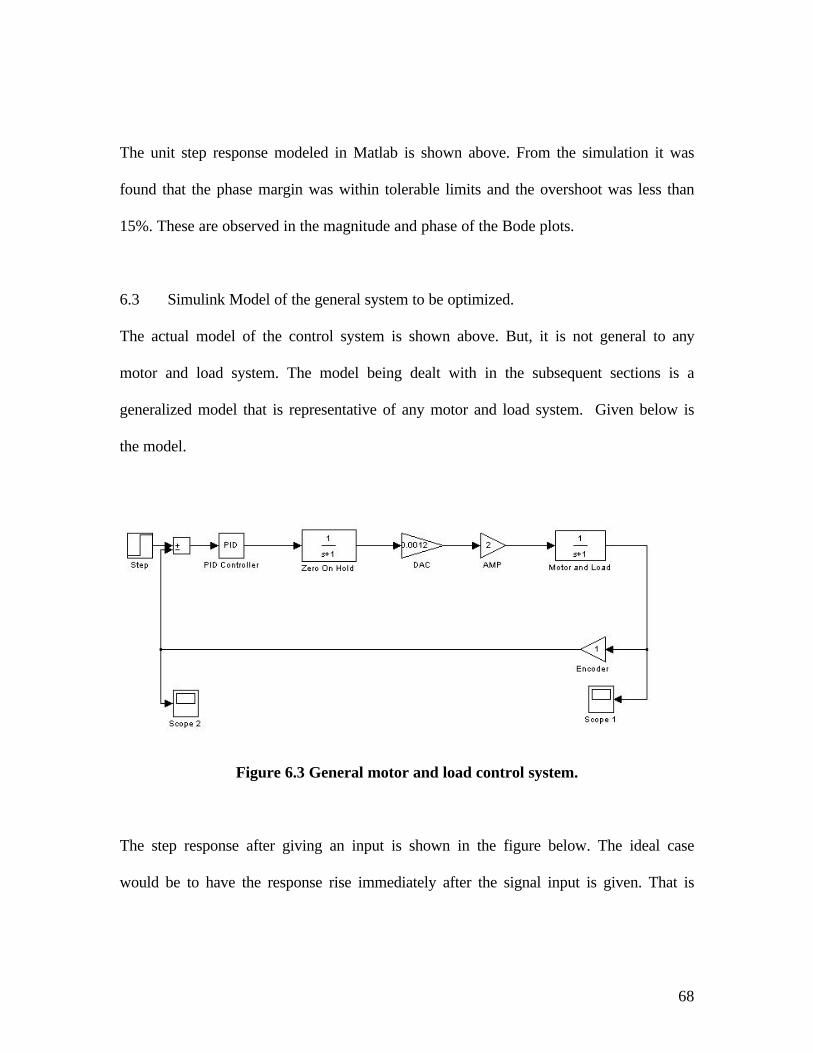
68

The unit step response modeled in Matlab is shown above. From the simulation it was

found that the phase margin was within tolerable limits and the overshoot was less than

15%. These are observed in the magnitude and phase of the Bode plots.

6.3 Simulink Model of the general system to be optimized.

The actual model of the control system is shown above. But, it is not general to any

motor and load system. The model being dealt with in the subsequent sections is a

generalized model that is representative of any motor and load system. Given below is

the model.

Figure 6.3 General motor and load control system.

The step response after giving an input is shown in the figure below. The ideal case

would be to have the response rise immediately after the signal input is given. That is

69

what one would like to achieve ideally. But depends of the components and parameters of

the system.

Time (seconds)

Figure 6.4 Step response of the system

6.4 Optimizing the control system to obtain PID values

The control parameters in the model above are optimized using a solver. This is a non-

linear model to be optimized. This would enable the system to track a unit step input to

the system with minimum error. MATLAB’s optimization toolbox is used to solve the

non-linear problem. The way this problem is tackled is in two steps. 1. The first method

minimizes the error between the output and the input signal using ‘lsqnonlin’ function 2.

The second method uses the ‘fminimax’ function. In this case, rather than minimizing the

error between the output and input the function minimizes the maximum value of the

output at any time. The variables are the parameters of the PID controller. If the error

70

needs to be minimized only at one time, it would be a single objective function. But, we

need to minimize the error for all time steps so it becomes a multiobjective function.

6.5 The lsqnonlin method

The routine lsqnonlin is used to perform a least square fit on the tracking of the output.

The following figure shows the error between the expected and the attained values at

several times.

Figure 6.5 Errors between desired and actual response at several times.

In the above figure E1,..E6 are the errors or difference between the input and output.

Ei = Input – Output

The objective would be to minimize the mean squared error , i.e.

71

Minimize

E = ∑=

N

iiE

N 1

21

The routine lsqnonlin is used to perform a least squares fit on the tracking of the output.

This is defined via a function in a separate M-file called ‘lsq.m’. It defines the error

signal. The function ‘lsq’ runs the simulation. Shown below is the file

Step 1: File lsq.m

function F = lsq(pid, a1, a2) Kp = pid(1); % Move variables into model parameters Ki = pid(2); Kd = pid(3); % choose solver and set model workspace to this function opt = simset('solver', 'ode5', 'SrcWorkspace', 'Current'); [tout, xout, yout] = sim('optsim', [0 100], opt); F = yout-1; % compute error signal

The simulink model file is specified in another M-file called the ‘optroutine’. The model

is the one shown above.

Step 2: File optroutine.m

kolmodel % loads the model pid0 = [1 10 12] % setting initial values a1 = 0; a2 = 0.0005; options = optimset('LargeScale', 'off', 'Display', 'iter', 'TolX', 0.001, 'TolFun', 0.001); pid = lsqnonlin('lsq', pid0, [], [], options, a1, a2) % put variables back into the base workspace Kp = pid(1); Ki = pid(2); Kd = pid(3);

72

First the variables Kp, Kd, Ki are all defined and initialized before calling ‘lsq’. When the

‘optroutine’ file is run the model is loaded and function ‘lsq’ does the optimization based

on the initial values of specified for the parameters and, constraints. A solver called

simset is chosen and the simulation is run using sim.

Finally the optimization gives the solution for the Proportinal, Integral, and Derivative

(Kp, Ki, Kd) gains of the controller after 55 function evaluations. The result from Matlab

is shown below.

pid0 =

1 5 10

Directional

Iteration Func-count Residual Step-size derivative Lambda

1 3 4.76719e+012 1 -4.91e+012

2 10 4.70723e+012 0.375 -1.51e+011 1.32032e+012

3 17 4.65431e+012 0.253 -2.33e+011 8.77204e+011

4 24 4.58281e+012 0.293 -8.38e+010 1.68981e+012

5 31 4.56367e+012 0.0868 -8.32e+010 2.02202e+012

6 39 4.53102e+012 0.119 -1.63e+011 2.60576e+012

7 55 4.53102e+012 3.28e-007 -3.27e+011 1.07078e+018

Optimization terminated successfully:

73

Search direction less than tolX

pid =

0.7234 4.9399 10.0233

The final optimized parameter values are,

Kp = 0.7235; Ki = 4.9399; Kd = 10.0233

Now, these optimized values are put into the PID block and the simulation is run. The

step response obtained is shown below.

Time (seconds)

Figure 6.6 Step response for using the optimized values.

The results are discussed in the subsequent chapter.

74

Chapter 7

Results and summary

The PID values obtained through the optimization method are the minimum mean square

error solution needed for the time response of the control system. This is because it tries

to minimize the error between the input and output. The step response plot using the

optimized value is also plotted. Optimized PID values are better as seen by comparing

both the plots.

In the graph using optimized values the signal rises to the required level faster (at time t =

200 using the optimized PID values, whereas at time t = 300 for starting values). Hence

the optimized values are definitely better than the previous values. It is also a better

alternative to the trial and error method used presently on the current robot. The method

is also more scientific and logical approach to a difficult problem of tuning the PID

controller.

The obtained values can be compared directly to the results obtained with the WSDK kit

to see the response of the system rather than trying iterative values. But, the kit can be

used to fine-tune the PID values after we arrive at the optimized value.

75

Chapter 8

Recommendations

Due the complex nature of framing the model, a generalized model was taken for

optimization. In future methods more work could be done to model actual control

systems for individual applications and be solved using the optimization routine. Even

though the iterative steps are eliminated, a better method for choosing the intial parameter

values should be developed.

This thesis deals with only one of the optimization methods but there are many more

methods to solve multi objective nonlinear problems. One of them is using a minmax

approach. More work could be directed toward that area where many routines are used on

the same problem and the best control parameters chosen. Based on those the software kit

can be used to fine-tune the values.

A stable testing platform, Bearcat II is available for testing. Various values can be used in

the program and the performance evaluated.

76

References

[1] M. F. Abdin, “An investigation of the potentials of Bi-directioanl AGV Systems,”

proc. 5th intl. AGVS conf., Tokyo, oct. 1987

[2] M. H. E. Larcombe, “Tracking Stability of Wire Guided Vehicles, “ proc. 1st Intl.

AGVS cong., pp. 137-144, 1973.

[3] Ozguner, Umit. Unyelioglu, Konur A. Hatipoglu, Cem. Analytical study of vehicle

steering control IEEE Conference on Control Applications - Proceedings 1995. IEEE,

Piscataway, NJ, USA,95CH35764.. p 125-130

[4] Ackermann, Juergen. Guldner, Juergen. Sienel, Wolfgang. Steinhauser, Reinhold.

Utkin, Vadim I. Linear and nonlinear controller design for robust automatic steering

IEEE Transactions on Control Systems Technology. v 3 n 1 Mar 1995. p 132-142

[5] Sung, Eric. Loon, Ng Kok. Yin, Yee Chiang. Parallel linkage steering for an

automated guided vehicle. IEEE Control Systems Magazine. v 9 n 6 Oct 1989 p 3-8

[6] Will, Anthony B. Zak, Stanislaw H. Modelling and control of an automated vehicle

Vehicle System Dynamics. v 27 n3 Mar 1997. p 131-155

[7] Zadeh, A Ghazi. Fahim, A. El-Gindy, M. Neural network and fuzzy logic applications

to vehicle systems: Literature survey International Journal of Vehicle Design. v 18 n 2

1997. p 132-193

77

[8] Kalyan Kolli and E.L. Hall. Steering Control System for a Mobile Robot Proceedings

of SPIE - The International Society for Optical Engineering. v 2591 1997. Society of

Photo-Optical Instrumentation Engineers, Bellingham, WA, USA.

[9] Kaylan Kolli, Sreeram Mallikarjun, Krishnamohan Kola and Ernest L. Hall. Speed Control for a Mobile Robot Proceedings of SPIE - The International Society for Optical

Engineering. v 2591 1997. Society of Photo-Optical Instrumentation Engineers,

Bellingham, WA, USA.

[10] Kamga, Andre. Rachid, Ahmed. Speed, steering angle and path tracking controls for

a tricycle robot Proceedings of the IEEE International Symposium on Computer-Aided

Control System Design 1996.,96TH8136.. p 56-61

[11] Tagawa, Y. Ogata, H. Morita, K. Nagai, M. Mori, H. Robust active steering system

taking account of nonlinear dynamics Vehicle System Dynamics. v 25 n Suppl 1996. p

668-681

[12] Matthews, Bradley O. Ruthemeyer, Michael A. Perdue, David. Hall, Ernest L.

Development of a mobile robot for the 1995 AUVS competition Proceedings of SPIE -

The International Society for Optical Engineering. v 2591 1995. Society of Photo-Optical

Instrumentation Engineers, Bellingham, WA, USA. p 194-201

[13] Samu, Tayib. Kelkar, Nikhal. Perdue, David. Ruthemeyer, Michael A. Matthews,

Bradley O. Hall, Ernest L. Line following using a two camera guidance system for a

mobile robot Proceedings of Spie - the International Society for Optical Engineering. v

2904 1996. p 290-297

78

[14] Yoshimoto, Ken-ichi. Sakatoh, Masatoshi. Takeuchi, Makoto. Ogawa, Hideki.

Automatic steering control algorithm using optical flow Jsae Review. v 16 n 2 Apr 1995.

p 165-169

[15] BenAmar, Faiz. Steering behaviour and control of fast wheeled robots IEEE

International Conference on Intelligent Robots and Systems. v 3 1997. IEEE, Piscataway,

NJ, USA,97CB36108. p 1396-1401

[16] Fourier, Cornelius J. Deist, Leon A. Control of a mobile robot by means of a fuzzy

algorithm

[17] Lucibello, Pasquale. State steering by learning for a class of nonlinear control

systems Automatica. v 30 n 9 Sept 1994. p 1463-1468

[18] Mori, Yasuchika. Nyudo, Shin. Steering and speed control of a car by fuzzy-neural

control Proceedings of the International Joint Conference on Neural Networks. Publ by

IEEE, IEEE Service Center, Piscataway, NJ, USA. v 2 1993. p 1753-1756

[19] Hattori, A. Kurami, K. Yamada, K. Ooba, K. Ueki, S. Nakano, E. Control system for

an autonomous driving vehicle Heavy Vehicle Systems. v 1 n 1 1993. p 99-113

[20] Hilton, J D. Hilton, D J. Design of an automatic steering and speed controller for a

horticultural gantry machine. National Conference Publication - Institution of Engineers,

Australia. Publ by IE Aust, Barton, Aust. n 92 pt 11. P 103-107

[21] Pears, N E. Bumby, J R. Steering control of an experimental autonomous vehicle.

Transactions of the Institute of Measurement & Control. v 13 n 4 1991 p 190-200

79

[22] Kehtarnavaz, N. Sohn, W. Steering control of autonomous vehicles by neural

networks. Proceedings of the American Control Conference. Publ by American

Automatic Control Council, Green Valley, AZ, USA (IEEE cat n 91CH2939-7). v 3. p

3096-3101

[23] Sawada, T. Oguchi, Y. Satoh, C. Basic study on the influence of aging on steering

control. Proceedings – Society of Automotive Engineers. Publ by SAE, Warrendale, PA,

USA. p 763-769

[24] Krogh, Bruce H. guaranteed steering control. Proceedings of the American Control

Conference 1985. Publ by IEEE, New York, NY, USA Available from IEEE Service

Cent (Cat. n 85CH2119-6), Piscataway, NJ, USA p 950-955

[25] McMahon, C B. Tennes, B R. Burkhardt, T H. performance results: microprocessor-

based steering controller using ultrasonic sensors. Paper - American Society of

Agricultural Engineers Joseph, Mich, USA 83-1568,. Publ by ASAE, St. 34p

[26] santina stubberd

[27] Warwick, K. Control systems : an introduction. New York : Prentice Hall, 1989

[28] Thompson, S. Control systems engineering and design. Harlow, Essex, England :

Longman Scientific & Technical ; New York, NY : Wiley, 1989

[29] Nise, Norman S. Control systems engineering / Norman S. Redwood City, Calif. :

Benjamin/Cummings Pub. Co., c1992

[30] I. J. Nagrath, M. Gopal. Control systems engineering New York : Wiley, c1975

80

[31] Charles L. Phillips, Royce D. Harbor. Basic feedback control systems. Englewood

Cliffs, N.J. : Prentice Hall, c1991

[32] Charles L. Phillips, Royce D. Harbor. Feedback control systems. Englewood Cliffs,

N.J. : Prentice Hall, c1991

[33] J. C. Gille, M. J. Pelegrin [and] P. Decaulne. Feedback control systems; analysis,

synthesis, and design New York, McGraw-Hill, 1959.

[34] Clarence J. Maday. Computer-aided design of feedback control systems for time

response. Research Triangle Park, N.C. : Instrument Society of America, c1987.

[35] Charles L. Phillips, H. Troy Nagle. Digital control system analysis and design.

Englewood Cliffs, N.J. : Prentice Hall, c1995.

[36] Mohammed S. Santina, Allen R. Stubberud, Gene H. Hostetter. Digital control

system design Fort Worth : Saunders College Pub., c1994.

[37] Benjamin C. Kuo. Digital control systems. Ft. Worth : Saunders College Pub.,

c1992.

[38] Alberto Isidori. Nonlinear control. Berlin ; New York : Springer, c1995.

[39] Alberto Isidori Nonlinear control systems : an introduction. Berlin ; New York :

Springer-Verlag, c1989.

[40] Cheng, R M H., Xiao, J W., LeQuoc, S., “Neuromorphic controller for AGV

steering,” Proceedings of the IEEE International Conference on Robotics and

Automation, IEEE, Piscataway, NJ, v 3. pp 2057-2062.

[41] Milacic, Vladimir R. Putnik, Goran D., “ Steering rules for AGV based on primitive

81

function and elementary movement control,” Robotics and Computer-Integrated

Manufacturing, v 5 n 2-3 1989. pp 249-254.

[43] Cheng, R M H. Rajagopalan, Ramesh. “Kinematics of automatic guided vehicles

with an inclined steering column and an offset distance, criterion for existence of inverse

kinematic solutions,” Journal of Robotic Systems, v 9 n 8 Dec 1992, pp 1059-1081.

[44] Ock Hyun Kim. Optimal Steering Control of an Auto-Guided-Vehicle with Two

Motored Wheels, Transactions of the Institute of Measurement & Control. v 9 n 2

Apr-Jun 1987, pp 58-63.

[45] P.F. Muir and C.P. Neuman, "Kinematic Modeling of Wheeled Mobile Robots,"

Journal of Robotic Systems, 4(2), 1987, pp. 281-340.

[46] E.L. Hall and B.C. Hall, Robotics: A User-Friendly Introduction, Holt, Rinehart,

and Winston, New York, NY, 1985, pp. 23.

[47] R.M.H. Cheng and R. Rajagopalan, "Kinematics of Automated Guided Vehicles

with an Inclined Steering Column and an Offset Distance: Criteria for Existence of

Inverse Kinematic Solution," Journal of Robotic Systems, 9(8), 1059-1081, Dec. 1992.

[48] General Electric, EV-1 SCR Control Manual, Charlottesville, Virginia 1986.

[49] Galil Inc, DMC-1000 Technical Reference Guide Ver 1.1, Sunnyvale, California

1993.

[50] Reliance Electric, Electro-Craft BDC-12 Instruction Manual, Eden Prairie,

Minnesota 1993.

[51] Fauver Corp., Parker Linear Actuators Catalog, Cincinnati, Ohio 1993.

82

[52] Delco Corp., Motor Specifications, Dayton, Ohio 1993.

[53] BEI Motion Systems Company, Model H20 Technical Specifications, Goleta,

California 1992

[54] Kalyan Kolli Chaktravarthy, Steering Control System Design and Analysis for an

Unmanned Autonomous Mobile Robot, Master’s Thesis, 1998.

[55] Krishnamohan Kola, Control System Design, Master’s Thesis, 1998.

[56] Math Works Inc., Matlab Control System Toolbox User’s Guide, 1996

[57] Math Works Inc., Matlab Optimization Toolbox, 1996

[58] VanDoren Vance J, “ Tuning Fundamentals – Basics of Proportional – Integral –

Derivative Control”, Control Engineering, March 1998.

[59] www.expertune.com/articles.html

83

Appendix

MATLAB code for the calculation of digital gains Section of code which takes in digital gains and converts them into analog gains GN=800

ZR=0.9

PL=0

KI=0

% Given GN...solve for K,A,B,C

K=GN;

A=ZR;

B=PL/256;

C=KI/8;

% solve for a,b,g,f

a=(2000-2000*A)/(1+A)

b=(2000-2000*B)/(1+B)

f=1000*C

g=K*(1+A)/(1+B)