1280-ch31 p 559. - ma.huji.ac.ilraumann/pdf/subjectivity and correlation.pdf · 31 subjectivity and...

31 Subjectivity and Correlation in Randomized Strategies

1 Introduction

Subjectivity and correlation, though formally related, are conceptually

distinct and independent issues. We start by discussing subjectivity.

A mixed strategy in a game involves the selection of a pure strategy by

means of a random device. It has usually been assumed that the random

device is a coin flip, the spin of a roulette wheel, or something similar;

in brief, an ‘‘objective’’ device, one for which everybody agrees on

the numerical values of the probabilities involved. Rather oddly, in spite

of the long history of the theory of subjective probability, nobody

seems to have examined the consequences of basing mixed strategies

on ‘‘subjective’’ random devices, i.e. devices on the probabilities of whose

outcomes people may disagree (such as horse races, elections, etc.).

Even a fairly superficial such examination yields some startling results, as

follows:

a. Two-person zero-sum games lose their ‘‘strictly competitive’’ charac-

ter. It becomes worthwhile to cooperate in such games, i.e. to enter into

binding agreements.1 The concept of the ‘‘value’’ of a zero-sum game

loses some of its force, since both players can get more than the value (in

the utility sense).

b. In certain n-person games with nZ 3 new equilibrium points appear,

whose payo¤s strictly dominate the payo¤s of all other equilibrium

points.2

Result (a) holds not just for certain selected 2-person 0-sum games, but

for practically3 all such games. Moreover, it holds if there is any area

whatsoever of subjective disagreement between the players, i.e., any event

in the world (possibly entirely unconnected with the game under consid-

eration) for which players 1 and 2 have di¤erent subjective probabilities.

The phenomenon enunciated in Result (b) shows that not only the 2-

person 0-sum theory, but also the non-cooperative n-person theory is

modified in an essential fashion by the introduction of this new kind of

strategy. However, this phenomenon cannot occur4 for 2-person games

This chapter originally appeared in Journal of Mathematical Economics 1 (1974): 67–96.Reprinted with permission.

1. Example 2.1 and sect. 6.

2. Example 2.3.

3. Specifically, wherever there is one payo¤ greater than the value and another one less thanthe value (for player 1, say).

4. Except in a very degenerate sense; see Example 2.2.

(zero-sum or not); for such games we will show5 that the set of equilib-

rium payo¤ vectors is not changed by the introduction of subjectively

mixed strategies.

We now turn to correlation. Correlated strategies are familiar from

cooperative game theory, but their applications in non-cooperative games

are less understood. It has been known for some time that by the use of

correlated strategies in a non-cooperative game, one can achieve as an

equilibrium any payo¤ vector in the convex hull of the mixed strategy

(Nash) equilibrium payo¤ vectors. Here we will show that by appropriate

methods of correlation, even points outside of this convex hull can be

achieved.6

In describing these phenomena, it is best to view a randomized strategy

as a random variable with values in the pure strategy space, rather than

as a distribution over pure strategies. In sect. 3 we develop such a frame-

work; it allows for subjectivity, correlation, and all possible combinations

thereof. Thus, a side product of our study is a descriptive theory (or

taxonomy) of randomized strategies.

We are very grateful to Professors M. Maschler, B. Peleg, and R. W.

Rosenthal for extremely stimulating correspondence and comments on

this study.

2 Examples

(2.1) Example Consider the familiar two-person zero-sum game

‘‘matching pennies,’’ which we write in matrix form as follows:

1; � 1 � 1; 1.

� 1; 1 1; � 1

Let D be an event to which players 1 and 2 ascribe subjective probability

2/3 and 1/3 respectively. Suppose now that the players bindingly agree to

the following pair of strategies: Player 2 will play left in any event; player

1 will play top if D occurs, and bottom otherwise. The expectation of

both players is then 1/3, whereas the value of the game is of course 0 to

both players.

To make this example work, one needs an event D whose subjective

probability is >1=2 for one player and <1=2 for the other. Such an event

5. Sect. 5.

6. Examples 2.5 through 2.9.

Strategic Equilibrium and the Theory of Knowledge560

can always be constructed as long as the players disagree about some-

thing, i.e., there is some event B with p1ðBÞ0 p2ðBÞ (where pi is the

subjective probability of i). For example, if p1ðBÞ ¼ 7=8 and p2ðBÞ ¼5=8, then we can construct the desired event by tossing a fair coin

twice (provided these particular coin tosses were not involved in the

description of B); if C is the event ‘‘at least one head,’’ then we have

p1ðBXCÞ ¼ 21=32 > 1=2 > 15=32 ¼ p2ðBXCÞ. This kind of construc-

tion can always be carried out (see the proof of Proposition 5.1).

(2.2) Example Suppose that there is an event D to which players 1 and

2 ascribe subjective probabilities 1 and 0 respectively and such that only

player 1 is informed before the play as to whether or not D occurs. Con-

sider the following pair of strategies: Player 2 plays left; player 1 plays

top if D occurs, bottom otherwise. This strategy yields a payo¤ of (1, 1);

moreover, it is actually in equilibrium, in the sense that neither player has

any incentive to carry out a unilateral change in strategy. However, it has

a somewhat degenerate flavor, since it requires that at least one of the

two players be certain of a falsehood (see sect. 8). We now show that a

similar phenomenon can also occur in a non-degenerate set-up; but it

requires 3 players.

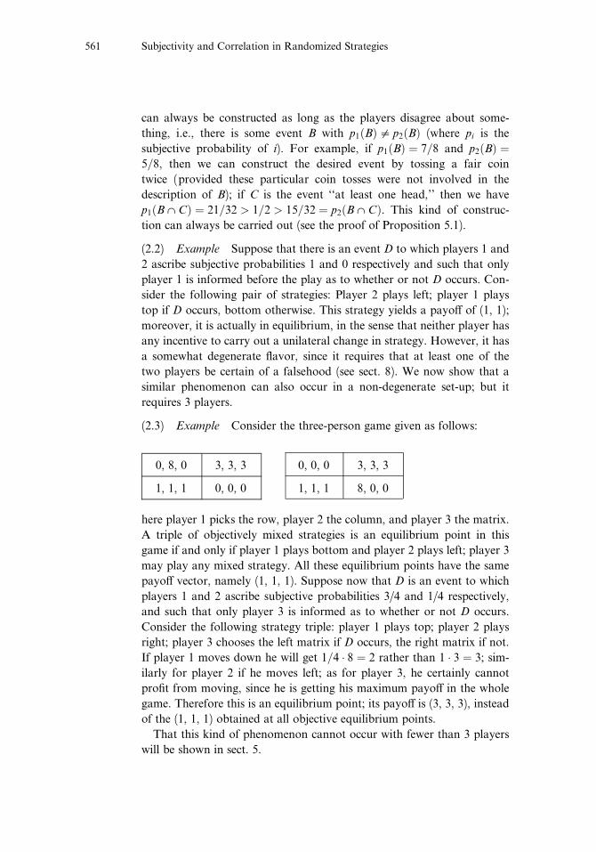
(2.3) Example Consider the three-person game given as follows:

0, 8, 0 3, 3, 3 0, 0, 0 3, 3, 3

1, 1, 1 0, 0, 0 1, 1, 1 8, 0, 0

here player 1 picks the row, player 2 the column, and player 3 the matrix.

A triple of objectively mixed strategies is an equilibrium point in this

game if and only if player 1 plays bottom and player 2 plays left; player 3

may play any mixed strategy. All these equilibrium points have the same

payo¤ vector, namely (1, 1, 1). Suppose now that D is an event to which

players 1 and 2 ascribe subjective probabilities 3/4 and 1/4 respectively,

and such that only player 3 is informed as to whether or not D occurs.

Consider the following strategy triple: player 1 plays top; player 2 plays

right; player 3 chooses the left matrix if D occurs, the right matrix if not.

If player 1 moves down he will get 1=4 � 8 ¼ 2 rather than 1 � 3 ¼ 3; sim-

ilarly for player 2 if he moves left; as for player 3, he certainly cannot

profit from moving, since he is getting his maximum payo¤ in the whole

game. Therefore this is an equilibrium point; its payo¤ is (3, 3, 3), instead

of the (1, 1, 1) obtained at all objective equilibrium points.

That this kind of phenomenon cannot occur with fewer than 3 players

will be shown in sect. 5.

Subjectivity and Correlation in Randomized Strategies561

An interesting feature of this example is that the higher payo¤ at the

new, subjective, equilibrium point is not only ‘‘subjectively higher,’’ it is

‘‘objectively higher.’’ That is, unlike the case in Example 2.1, the payo¤ is

higher not only because of the di¤ering probability estimates of the play-

ers, but it is higher in any case, whether or not the event D takes place.

The contribution of subjective probabilities in this case is to make the

new point an equilibrium; once chosen, it is sure to make all the players

better o¤ than at any of the old equilibrium points.

We remark that by using di¤erent numbers we can find similar exam-

ples based on arbitrarily small probability di¤erences.

It is essential in this example that only player 3 be informed as to

whether or not D occurs. If, say, player 1 were also informed (before the

time comes for choosing his pure strategy), he could do better by playing

top or bottom according as to whether D occurs on not.7 This secrecy

regarding D is quite natural. If we were to insist that all players be

informed about D, it would be like insisting that in an objectively mixed

strategy based on a coin toss, all players be informed as to the outcome

of the toss. But much of the e¤ectiveness of mixed strategies is based

precisely on the secrecy, which would then be destroyed. In practical sit-

uations, it is of course quite common for some players to have di¤ering

subjective probabilities for events about which they are not informed, and

on which other players peg their strategy choices.

Our last 6 examples deal with correlation.

(2.4) Example Consider the following familiar 2-person non-zero-sum

game:

2; 1 0; 0.

0; 0 1; 2

There are exactly 3 Nash equilibrium points: 2 in pure strategies, yielding

(2, 1) and (1, 2) respectively, and one in mixed strategies, yielding (2/3, 2/3).

The payo¤ vector (3/2, 3/2) is not achievable at all in (objectively) mixed

strategies. It is, however, achievable in ‘‘correlated’’ strategies, as follows:

One fair coin is tossed; if it falls heads, players 1 and 2 play top and left

respectively; otherwise, they play bottom and right.

The interesting aspect of this procedure is that it not only achieves

(3/2, 3/2), it is also in equilibrium; neither player can gain by a unilateral

change. Any point in the convex hull of the Nash equilibrium payo¤s of

7. I am grateful to R. W. Rosenthal for this remark.


any game can be achieved in a similar fashion, and will also be in equi-

librium. This is not new; it has been in the folklore of game theory for

years. I believe the first to notice this phenomenon (at least in print) were

Harsanyi and Selten (1972).

In the following 4 examples we wish to point out a phenomenon that

we believe is new, namely that by the use of correlated strategies one can

achieve a payo¤ vector that is in equilibrium in the same sense as above,

but that is outside the convex hull of the Nash equilibrium payo¤s. In

fact, except in Example 2.7, it is better for all players than any Nash

equilibrium payo¤.

(2.5) Example Consider the 3-person game given as follows:

0, 0, 3 0, 0, 0 2, 2, 2 0, 0, 0 0, 0, 0 0, 0, 0.

1, 0, 0 0, 0, 0 0, 0, 0 2, 2, 2 0, 1, 0 0, 0, 3

Here player 1 picks the row, player 2 the column, and player 3 the

matrix. If we restrict ourselves to pure strategies, there are only 3 equi-

librium payo¤s, namely (0, 0, 0), (1, 0, 0), and (0, 1, 0). If we allow

(objectively) mixed strategies, some more equilibrium payo¤s are added,

but none of their coordinates exceed 1. Consider now the following strat-

egy triple: Player 3 plays the middle matrix. Players 1 and 2 get together

and toss a fair coin, but do not inform player 3 of the outcome of the

toss. If the coin falls on heads, players 1 and 2 play top and left respec-

tively; otherwise, they play bottom and right respectively. The payo¤ is

(2, 2, 2). If player 3 would know the outcome of the toss, he would be

tempted to move away; for example, if it was heads, he would move left.

Since he does not know, he would lose by moving. Thus the introduction

of correlation among subsets of the players can significantly improve the

payo¤ to everybody.

(2.6) Example Another version of Example 2.5 is the following:

0, 1, 3 0, 0, 0 2, 2, 2 0, 0, 0 0, 1, 0 0, 0, 0.

1, 1, 1 1, 0, 0 2, 2, 0 2, 2, 2 1, 1, 1 1, 0, 3

This version has the advantage that there is only one Nash equilibrium

payo¤, namely (1, 1, 1); and it can be read o¤ from the matrices by the

use of simple domination arguments, as compared to the slightly labori-

ous computations needed in the previous example. The advantage of


Example 2.5 is that the new correlated strategy equilibrium point has the

property that any deviation will actually lead to a loss (not only a failure

to gain).

In both examples, player 3 will not even want to know the outcome of

the toss; he will want players 1 and 2 to perform it in secret. It is impor-

tant for him that players 1 and 2 know that he does not know the out-

come of the toss; otherwise they cannot depend on him to choose the

middle matrix, and will in consequence themselves play for an equilib-

rium point that is less advantageous for all. Thus in Example 2.6, player

3 knows that if he can ‘‘peep,’’ then players 1 and 2 will necessarily play

bottom and left respectively, to the mutual disadvantage of all.

(2.7) Example In Examples 2.5 and 2.6, equilibrium payo¤s outside of

the convex hull of the Nash equilibrium payo¤s were achieved by ‘‘par-

tial’’ correlation—correlation of strategy choices by 2 out of the 3 play-

ers. We now show that a similar phenomenon can occur even in 2-person

games; here again a kind of partial correlation is used, but it is subtler

than that appearing previously.

Consider the 2-person game given as follows:

6; 6 2; 7.

7; 2 0; 0

This game has two pure strategies equilibrium points, with payo¤ (2, 7)

and (7, 2) respectively, and one mixed strategy equilibrium point, with

payo¤ (4 23, 4 2

3). Consider now an objective chance mechanism that

chooses one of three points A, B, C with probability 1/3 each. After the

point has been chosen, player 1 is told whether or not A was chosen, and

player 2 is told whether or not C was chosen; nothing more is told to the

players. Consider the following pair of strategies: If he is informed that A

was chosen, player 1 plays his bottom strategy; otherwise, his top strat-

egy. Similarly, if he is informed that C was chosen, player 2 plays

his right strategy; otherwise, he goes left. It is easy to verify that this

pair of strategies is indeed in equilibrium, and that it yields the players an

expectation of (5, 5)—a payo¤ that is outside the convex hull of the Nash

equilibrium payo¤s (listed above).

The strategies in this equilibrium point are not stochastically indepen-

dent, like the mixed or pure strategies appearing in Nash equilibrium

points, nor are they totally correlated, like the strategies appearing in

Example 2.4. It is precisely the partial correlation that enables the phe-

nomenon we observe here.


(2.8) Example Consider the 2-person game given as follows:

6; 6 0; 0 2; 7

0; 0 4; 4 3; 0 .

7; 2 0; 3 0; 0

This is obtained from the previous example by adding a middle row and

a middle column, with appropriate payo¤s. The strategy pairs (top, right)

and (bottom, left), which previously yielded the equilibrium payo¤s (2, 7)

and (7, 2), are no longer in equilibrium; the equilibrium property has

been ‘‘killed’’ by the addition of the new strategies. The mixed-strategy

pair which previously yielded (4 23, 4

23) remains in equilibrium here; more-

over we get a new pure strategy equilibrium point yielding (4, 4), and a

new mixed strategy equilibrium point yielding (2 1023, 2

1023). These are all the

Nash equilibrium payo¤s. Thus we see that 4 23 is the maximum that

either player can get at any Nash equilibrium point.

The equilibrium point in ‘‘partially correlated’’ strategies described in

Example 2.7 remains in equilibrium here, and yields (5, 5)—more, for

both players, than that yielded by any of the Nash equilibria.

Though the random device needed in Examples 2.7 and 2.8 is con-

ceptually somewhat more complex than the coin tosses (secret or joint)

used in classical game theory and in Examples 2.4, 2.5, and 2.6, it is not

at all di‰cult to construct. Given a roulette wheel, it is easy to attach

electrical connections that will do the job. If the reader wishes, he can

think of the players as jointly supervising the construction of the device,

and then retiring to separate rooms to get the information and choose

their strategies. It is advantageous for both players to build the device, to

satisfy each other that it is working properly, and then to follow the

above procedure. Once chosen, the procedure is of course self-enforcing;

neither player will wish to renege at any stage.

(2.9) Example Consider again the 2-person 0-sum game ‘‘matching

pennies’’ already treated in Example 2.1. Suppose that nature chooses

one of four points A, B, C, or D, and that players 1 and 2 ascribe to these

choices subjective probabilities (1/3, 1/6, 1/6, 1/3) and (1/6, 1/3, 1/3, 1/6),

respectively. Under no condition is either player told which point was

chosen, but player 1 is told whether the point chosen is in fA;Bg or in

fC;Dg, and player 2 is told whether the point chosen is in fA;Cg or in

fB;Dg. Consider the following strategy pair: Player 1 chooses top or

bottom according as to whether he is told ‘‘fA;Bg’’ or ‘‘fC;Dg’’; player2 chooses left or right according as to whether he is told ‘‘fA;Cg’’ or


‘‘fB;Dg.’’ Like the strategy pair in Example 2.1, this yields each player

an expectation of 1/3, whereas the value of the game is of course 0 to both

players; unlike the strategy pair of Example 2.1, this pair is in equilibrium.

If, in a 2-person zero-sum game with value v, we permit correlation

but rule out subjectivity, then the payo¤s to all strategy pairs continue

to sum to 0, and it is easy to see that the only equilibrium points have

payo¤s ðv;�vÞ. If we rule out correlation (i.e. permit mixed or pure

strategies only) but permit subjectivity, we still get only ðv;�vÞ as an

equilibrium payo¤; this follows from Proposition 5.1. But if we permit

both subjectivity and correlation, then this example shows that there

may exist mutually advantageous equilibrium points, even in 2-person

0-sum games.

3 The Formal Model

In this section, definitions are indicated by italics.

A game consists of:

1. a finite set N (the players); write N ¼ f1; . . . ; ng;2. for each i A N, a finite set Si (the pure strategies of i );

3. a finite set X (the outcomes);

4. a function g from the cartesian product S ¼ xi A nSi onto X (the out-

come function).

This completes the description of the game as such; formally, however,

we still need some equipment for randomizing strategies, and for defining

utilities and subjective probabilities for the players. Thus to the descrip-

tion of the game we append the following:

5. A set W (the states of the world), together with a s-field B of subsets of

W (the events);

6. For each player i, a sub-s-field Ii of B (the events in Ii are those

regarding which i is informed).

7. For each player i, a relation xi (the preference order of i ) on the

space of lotteries on the outcome space X, where a lottery on X is a B-

measurable8 function from W to X.

The intuitive scenario associated with this model involves the following

steps, to be thought of as occurring one after the other as follows:

8. This means that for each x A X , the set {x ¼ x} [i.e. the set {o: xðoÞ ¼ x}] is in B.


i. Nature chooses a point o in W.

ii. Each player i is informed as to which events in Ii contain o.

iii. Each player i chooses9 a pure strategy si in Si.

iv. The outcome is determined10 to be gðs1; . . . ; snÞ.

Returning to the formal model, let us define a randomized strategy (or

simply strategy) for player i to be a measurable function si from (W;Ii) to

Si. Note that si must be measurable w.r.t. (with respect to) Ii, not merely

w.r.t. B; this means that i can peg his strategies only on events regarding

which he is informed. [In the above scenario, strategies are chosen before

step (ii).]

If s is an n-tuple of strategies, then gðsÞ is a lottery on X. An equilib-

rium point is an n-tuple s ¼ ðs1; . . . ; sn) of strategies such that for all i and

all strategies ti of i, we have

gðsÞxi gðs1; . . . ; si�1; ti; siþ1; . . . ; snÞ:

We will assume:

assumption I For each i, there is a real function ui on X (the utility

function of i ) and a probability measure11 pi on W (the subjective

probability of i) such that for all lotteries x and y on X, we have

xxi y if and only ifðW

uiðxðoÞÞdpiðoÞZðW

uiðyðoÞÞdpiðoÞ;

moreover, pi is unique.12

This assumption says that player i ’s preferences between lotteries are

governed by the expected utility of the outcomes of the lotteries. There

are well known systems of axioms on the preferences xi that lead to

utilities and subjective probabilities; see for example Savage (1954) or

Anscombe and Aumann (1963).

Note that pi is defined on all of B, not only on Ii; that is, i assigns a

probability to all events, not only those regarding which i is informed.

9. Without informing the other players.

10. Note that g does not depend on o; see subsect. (d) of sect. 9.

11. s-additive non-negative measure with piðWÞ ¼ 1.

12. I.e. if (u0i; p0i) also satisfy the condition of the previous sentence, then p0i ¼ pi. Axiom

systems leading to subjective probabilities usually imply the uniqueness as well. In our case,if we had wanted to minimize our assumptions we could have avoided assuming uniqueness,at this stage. Indeed, the uniqueness of pi follows from the existence of a non-atomic pi ; andthis is assumed in Assumption II. It is, however, more convenient to assume uniquenessalready at this stage, since it enables us to refer immediately to ‘‘the’’ subjective probabilityof player i, and this simplifies the entire discussion.


Two events A and B are i-independent if

piðAXBÞ ¼ piðAÞpiðBÞ;

intuitively, this means that i can get no hint about A from information

regarding B. More generally, the events A1; . . . ;Ak are i-independent if

piðB1 X � � � XBkÞ ¼ piðB1Þ � � � piðBkÞ

whenever each Bj is either Aj or W. Events are independent if they are i-

independent for all i. An event is i-secret if it is in Ii, and for each j other

than i, it is j-independent of all events in the s-field generated by all the

Ik with k0 i. Thus i is informed regarding each i-secret event, but play-

ers other than i can get no hint of it, even by pooling their knowledge.

The family of i-secret events is denoted Si. We assume

assumption II For each i, there is a s-field Ri of i-secret events such

that each pj is non-atomic on Ri.

Intuitively, Ri an be constructed from a roulette spin conducted by i in

secret. To obtain the non-atomicity, it is su‰cient to assume that each

player j assigns subjective probability 0 to each particular outcome;13 or

equivalently, that there exist finite partitions of W into Ri-events whose

pj-probabilities are arbitrarily small. Such non-atomicity assumptions are

familiar in treatments of subjective probability.14 Note that the roulette

wheel need not be ‘‘objective,’’ i.e. the players may disagree about the

probabilities involved.

A strategy si of i is mixed if it is Si-measurable, i.e. pegged on i-secret

events. Strategies s1; . . . ; sn are uncorrelated if for each s A S, the n events

fsj ¼ sjg are independent. Mixed strategies are uncorrelated, but the

converse is false; strategies may be uncorrelated even though they are

pegged on events regarding which all players are informed.

An event A is called objective if all the subjective probabilities piðAÞcoincide; in that case their common value is called the probability of A,

and is denoted pðAÞ. A strategy si of i is called objective if it is pegged on

objective events, i.e. if fsi ¼ sig is an objective event for all si A Si. The

strategies occurring in the classical non-cooperative theory are precisely

those that are both objective and mixed.

An event or strategy is called subjective if it is not objective.

The preference order of i determines his utility function on X only up

to a monotonic linear transformation. Given a specific choice u1; . . . ; unof utility functions of the players, define the payo¤ function of player i in

13. The set of outcomes is taken to be the unit interval (not {0; 1; . . . ; 36}).

14. Cf. Savage (1954, pp. 38–40, especially postulates P60 and P6).


the usual way; that is, if s is an n-tuple of pure strategies (i.e. s A S),

define

hiðsÞ ¼ uiðgðsÞÞ;

and if s is an n-tuple of arbitrary strategies, define

HiðsÞ ¼ EiðhiðsÞÞ ¼ðW

hiðsðoÞÞdpiðoÞ; ð3:1Þ

Ei being the expectation operator w.r.t. the probability measure pi on W.

Then gðsÞti gðtÞ if and only if HiðsÞ > HiðtÞ. Write

h ¼ ðh1; . . . ; hnÞ;

H ¼ ðH1; . . . ;HnÞ:

Any vector of the form HðsÞ is called a feasible payo¤; if s is an equilib-

rium point, then HðsÞ is called an equilibrium payo¤; and if s is an equi-

librium point in objective mixed strategies, then HðsÞ is an objective

mixed equilibrium payo¤.

To orient the reader, we mention that Example 2.1 involves a pair of

subjective strategies that is not in equilibrium; Examples 2.2 and 2.3

involve equilibrium points in mixed subjective strategies; and

Examples 2.4 through 2.8 involve equilibrium points that are objective,

but are not in mixed strategies (the strategies are in fact correlated, i.e.

not uncorrelated).

4 Preliminaries and Generalities

This section is devoted to the statement of several lemmas needed in the

sequel, of an existence theorem for equilibrium points (Proposition 4.3),

and of a proposition concerning the nature of the sets of feasible and

equilibrium payo¤s. We also discuss the notion of ‘‘correlation.’’

Though most of the results stated in this section are intuitively unsur-

prising, the proofs are a little involved (because of the relatively weak

assumptions we have made). We therefore postpone these proofs to sect. 7,

in order to get as quickly as possible to the conceptually more interesting

results of the paper (Propositions 5.1 and 6.1). Readers who are inter-

ested only in the statements of these propositions (as opposed to the

proofs) may skip this section.

The first lemma asserts that objective mixed strategies can be con-

structed with arbitrary probabilities, i.e. that all the ‘‘classical’’ mixed

strategies appear in this model as well. Define a distribution on Si to be a

real-valued function on Si whose values are non-negative and sum to 1.


(4.1) lemma Let i A N, and let si be a distribution on Si. Then i has an

objective mixed strategy si such that for all si A Si,

pfsi ¼ sig ¼ siðsiÞ:

Next, we have

(4.2) lemma For any i in N, any event B, and any a between 0 and 1,

there is an objective i-secret event with probability a that is independent

of B.

Intuitively, Lemmas 4.1 and 4.2 depend on the existence of an objective

roulette wheel that i can spin in secret. Thus they appear to go somewhat

further15 than Assumption II, and it is of some interest that in fact, they

follow from it.

The next proposition asserts that the classical equilibrium points of

Nash (1951) appear in this model as well. If s ¼ ðs1; . . . ; snÞ is an n-tuple

of distributions on S1; . . . ;Sn respectively, and if i A N, define

FiðsÞ ¼ SshiðsÞPj A NajðsjÞ;

where the sum runs over all pure strategy n-tuples s ¼ ðs1; . . . ; snÞ. Thepayo¤ to s is the n-tuple FðsÞ ¼ ðF1ðsÞ; . . . ;FnðsÞÞ. Recall that s is a

Nash equilibrium point if for any i and any distribution ti on Si, we have

FiðsÞZFiðs1; . . . ; si�1; siþ1; . . . ; snÞ;

in that case F ðsÞ is called a Nash equilibrium payo¤.

(4.3) proposition The set of Nash equilibrium payo¤s coincides with

the set of objective mixed equilibrium payo¤s.

From this proposition and Nash’s theorem it follows immediately that

there is an equilibrium point in every game.

We now come to the concept of correlation. Set SN ¼ 7i A N

Ii; the

members of SN are called public events. A continuous chance device, or

roulette for short, is a sub-s-field R of W on which each pj is non-atomic;

if R consists of public events, it is called a public roulette.

Parallel to Lemma 4.2, we have

(4.4) lemma Assume that there is a public roulette. Then for any event

B, and any a between 0 and 1, there is an objective public event with prob-

ability a that is independent of B.

15. See subsection (e) of sect. 9 for a discussion of this point.


A public roulette can be used as a correlating device on which all

players can peg their choices; this leads (cf. Example 2.4) to

(4.5) proposition Assume that there is a public roulette. Then the set of

equilibrium payo¤s and the set of feasible payo¤s are both convex.

It is not known whether the set of equilibrium—or feasible—payo¤s is

closed, whether or not one assumes the existence of a public roulette.

Public roulettes enable all players to correlate their strategies, as in

Example 2.4. In Examples 2.5 through 2.9, the correlation is of a subtler

kind. To describe the situation, let us call the triple consisting of the pair

(W;BÞ, the n-tuple (I1; . . . ;In), and the n-tuple (p1; . . . ; pn) a randomiz-

ing structure. In Examples 2.4, 2.5, and 2.6, the randomizing structure is

of a particularly simple kind, which we call standard, and which is de-

scribed as follows:

For each T HN, let JT be a copy of the unit interval [0, 1] with the

Borel sets. Let ðW;BÞ ¼ xT HNJT , and let pT be the projection of W on

JT . For i in N, call two members o1 and o2 of W i-equivalent if

pTðo1Þ ¼ pTðo2Þ for all T containing i. Let Ii be the s-field of all events

in W that are unions of i-equivalence classes. Let all the pi be Lebesgue

measure on W.

Intuitively, the points of JT are outcomes of an objective roulette spin

conducted in the presence of the members of T only. Note that all the

probabilities are the same, so that subjectivity does not enter the picture.

Even in this relatively simple case, though, it is not clear that the set of

equilibrium payo¤s is closed (it is convex by Proposition 4.5). However,

when n ¼ 2 and the randomizing structure is standard, then it is easily

verified that the set of equilibrium payo¤s is precisely the convex hull of

the Nash equilibrium payo¤s.

In Example 2.7, the randomizing structure is not standard; but the

probabilities are objective, i.e. all the pi coincide. It is easily verified that

whenever the probabilities are objective and there is a public roulette, the

set of feasible payo¤s is simply the convex hull of the pure strategy pay-

o¤s. In particular, this will be the case when the randomizing structure is

standard.

5 Equilibrium Points in Two-Person Games

In Example 2.3 we showed that by pegging strategies on subjective

events, it is possible to find a 3-person game with an equilibrium point in

mixed strategies whose payo¤ is higher for all players than the payo¤ to


any equilibrium in objective mixed strategies. In this section we show that

this cannot happen in the case of 2-person games.

(5.1) proposition Let G be a 2-person game,16 and assume that

for any event B; p1ðBÞ ¼ 0 if and only if p2ðBÞ ¼ 0: ð5:2Þ

Then for each equilibrium point s in mixed strategies, there is an equilib-

rium point t in objective mixed strategies such that HðsÞ ¼ HðtÞ.

Proof Let (s1; s2) be an equilibrium point in mixed strategies. Let t1 be

an objective mixed strategy for player 1 that mimics the way player 2 sees

s1, i.e., such that for all pure strategies s1 of player 1,

pft1 ¼ s1g ¼ p2fs1 ¼ s1g; ð5:3Þ

such a strategy exists because of Lemma 4.1. Similarly, let t2 be an

objective mixed strategy for player 2 such that for all s2,

pft2 ¼ s2g ¼ p1fs2 ¼ s2g: ð5:4Þ

Let s11; s12; . . . be the pure strategies that enter actively into s1, i.e., with

positive p1-probability. Because s1 is in equilibrium,

E1h1ðs1j ; s2Þ ¼ H1ðs1; s2Þ ð5:5Þ

for all j. But from (5.2) it follows that the s1j are also precisely the pure

strategies that enter actively into t1; hence (5.5) yields

H1ðt1; s2Þ ¼ H1ðs1; s2Þ: ð5:6Þ

Since s1 maximizes H1 (if 2 plays s2), it follows from (5.6) that t1 also

does. But by (5.4), player 1 ascribes the same distribution to t2 as to s2;

therefore

H1ðt1; t2Þ ¼ H1ðt1; s2Þ ¼ H1ðs1; s2Þ;

and furthermore, t1 maximizes H1 if 2 plays t2. Similarly,

H2ðt1; t2Þ ¼ H2ðs1; t2Þ ¼ H2ðs1; s2Þ;

and t2 maximizes H2 if 1 plays t1. Therefore (t1; t2) is an objective mixed

equilibrium point with the same payo¤ as (s1; s2), and the proof of this

proposition is complete.

It would have been reasonable to conjecture that this proposition

remains true if both occurrences of the word ‘‘mixed’’ are deleted.

Example 2.9 shows that this is false.

16. Not necessarily 0-sum.


6 Two-Person Zero-Sum Games

A game is called 2-person 0-sum if n ¼ 2 and if there are utility functions

u1 and u2 for the players such that

u1ðxÞ þ u2ðxÞ ¼ 0

for all x A X . After adopting a specific such pair of utility functions, one

defines the value of the game as usual. Specifically, Proposition 4.3 pro-

vides an equilibrium point in objective mixed strategies; by the minimax

theorem, all such equilibrium points must have the same payo¤, which is

of the form ðv;�vÞ. Then v is called the value of the game.

(6.1) proposition Let G be a 2-person 0-sum game with value v.

Assume that

there are outcomes x and y with u1ðxÞ > v > u1ðyÞ; and ð6:2Þ

for each player i; there is a subjective event Bi regarding which i

is informed: ð6:3Þ

Then there is a pair s of strategies such that

H1ðsÞ > v;H2ðsÞ > �v: ð6:4Þ

Remark The proposition is considerably easier to prove if one assumes

that

there is a public subjective event B and there is a public roulette. (6.5)

To see this, assume without loss of generality that p1ðBÞ > p2ðBÞ (other-wise, use the complement of B). If C is a public event and 0Y yY 1,

denote by yC a public event such that

p1ðyCÞ ¼ yp1ðCÞ and p2ðyCÞ ¼ yp2ðCÞ;

the existence of such a yC follows17 from Lemma 4.4. From (6.2) it

follows that there is a b with 0 < b < 1 such that

v ¼ bu1ðxÞ þ ð1� bÞu1ðyÞ:

For 0 < d < 1, set

Bd ¼ WndðWnBÞ:

17. It also follows from the theorem of Lyapunov (1940) on the range of a vector measure.We shall see in sect. 8 that Proposition 4.4 is itself proved via Lyapunov’s theorem; intui-tively, though, Proposition 4.4 is more transparent than Lyapunov’s theorem.


Then for d su‰ciently small, we have p1ðBdÞ > p2ðBdÞ > b; hence if we

let A ¼ yBd for an appropriate y, then

p1ðAÞ > b > p2ðAÞ: ð6:6Þ

Now define s as follows: Both players choose pure strategies leading

to x, or both players use pure strategies leading to y, according as to

whether A does or does not occur. Then (6.4) follows, and the proposi-

tion is proved under the assumption of (6.5).

Proof of Proposition 6.1 In (6.2), let x ¼ gðr1; r2Þ and y ¼ gðt1; t2Þ; then

h1ðr1; r2Þ > v > h1ðt1; t2Þ:

Suppose first that h1ðr1; t2ÞZ v. Setting

H�ðeÞ ¼ eh1ðr1; r2Þ þ ð1� eÞh1ðr1; t2Þ

H�ðeÞ ¼ eh1ðt1; r2Þ þ ð1� eÞh1ðt1; t2Þ;

we find that for e > 0 su‰ciently small,

H�ðeÞ > v > H�ðeÞ:

Hence there is a b in [0, 1] with

v ¼ bH�ðeÞ þ ð1� bÞH�ðeÞ:

Now let A1 be a subjective event in I1 with p1ðA1Þ > b > p2ðA1Þ. Theexistence of such an event may be established as in the remark [cf. (6.6)],

except that now the mapping C ! yC takes I1 into itself (rather than

I1 XI2 into itself ), Lemma 4.2 (rather than 4.4) is used to prove the

existence of yC, and B1 is substituted for B. Again using Lemma 4.2, we

obtain an objective 2-secret event A2 with probability e that is indepen-

dent of A1. Define a strategy pair s by stipulating that si takes the value rior ti according as to whether Ai does or does not occur. Then s is uncor-

related and satisfies (6.4).

If h1ðr1; t2ÞY v, the proof is similar, the roles of the two players being

then reversed. This completes the proof of Proposition 6.1.

Proposition 6.1 fails if it is only assumed that there is a subjective event

of which at least one player is informed. For example, if in the 2-person

0-sum game with matrix

1 1,

2 0


there is a subjective event in I1 but not in I2, then there is no pair of

strategies satisfying (6.4). In this game it is su‰cient for (6.4) that there

be a subjective event in I2. In general, the proof of Proposition 6.1 shows

that in any specific game, only one player need use a subjective strategy,

while the other can use an objective one; but which player it is that uses

the subjective strategy may depend on the game.

It is perhaps worth noting that in Proposition 6.1, the strategies con-

stituting s may be taken to be independent; indeed, the strategies con-

structed in the proof are independent.

7 Proof of the Propositions of Sect. 4

We start with a lemma that is basic to the proofs in this section.

(7.1) lemma Let R be a roulette, and let B1; . . . ;Bl be events. Then for

any a between 0 and 1, there is an objective event in R with probability a

that is independent of each of the Bk.

Proof Consider the ð1þ lÞn-dimensional vector measure u on (W;R)

defined by

miðAÞ ¼ piðAÞ; i ¼ 1; . . . ; n;

mknþiðAÞ ¼ piðAXBkÞ; i ¼ 1; . . . ; n; k ¼ 1; . . . ; l:

That m is non-atomic follows from the non-atomicity of the pi on R. By

the theorem of Lyapunov (1940) on the range of a vector measure, the

range of m is convex. Now

mðWÞ ¼ ð1; . . . ; 1; p1ðB1Þ; . . . ; pnðB1Þ; . . . ; p1ðBlÞ; . . . ; pnðBlÞÞ

and

mðfÞ ¼ ð0; . . . ; 0Þ:

Hence amðWÞ is in the range of m, i.e. there is a set A in R such that

mðAÞ ¼ amðWÞ. This means that piðAÞ ¼ a for all i and

piðAXBkÞ ¼ apiðBkÞ ¼ piðAÞpiðBkÞ

for all i. The proof of the lemma is complete.

Proof of Lemma 4.1 By induction on the number m of members si of Si

for which siðsiÞ > 0. Let Ri be the i-secret roulette provided by Assump-

tion II. As often in the case of inductive proofs, it is convenient to prove

a somewhat stronger statement than is needed; here we show that


a strategy s1 can be chosen obeying Proposition 4:1; so that the

events fsi ¼ sig are in R1: ð7:2Þ

If m ¼ 1 there is nothing to prove. Let m > 1, and suppose the proposi-

tion true for m� 1. Let Si ¼ fs1i ; . . . ; smi ; . . .g, where siðs ji Þ > 0 if and

only if jYm. By the induction hypothesis, there are disjoint objective

events B1; . . . ;Bm�1 such that pðBjÞ ¼ siðs ji Þ=ð1� siðsmi ÞÞ. By Lemma 7.1

with R ¼ Ri, there is an objective i-secret event Bm independent of each

of B1; . . . ;Bm�1, such that pðBmÞ ¼ 1� siðsmi Þ. Set Aj ¼ Bj XBm for

j < m, Am ¼ WnBm, and Aj ¼ f for j > m; then Aj A Ri for all j. Define

si by siðoÞ ¼ sji if and only if o A Aj. Then si satisfies (7.2). This com-

pletes the proof of Lemma 4.1.

Proof of Lemma 4.2 Use Assumption II, and apply Lemma 7.1 with

R ¼ Ri and l ¼ 1.

Before proving Proposition 4.3 we need a lemma.

(7.3) lemma Let (s1; . . . sn) be an n-tuple of strategies, and let s A S. For

some i A N, suppose that all the sj except possibly si are mixed. Then

pifs ¼ sg ¼ pifsi ¼ sigpifsj ¼ sj for all j0 ig

¼ pifs ¼ s1g . . . pifsn ¼ sng:

Proof W.l.o.g. let i ¼ 1, and let Aj ¼ fsj ¼ sjg for all j; then

fs ¼ sg ¼ A1 X � � � XAn:

Moreover, A1 A I1 and Aj A Si for j > 1. By definition of Sj, each Aj

with j > 1 is 1-independent of Ajþ1 X � � � XAn. Hence

p1ðA2 X � � � XAnÞ ¼ p1ðA2Þp1ðA3 X � � � XAnÞ

¼ � � � ¼ p1ðA2Þ � � � p1ðAnÞ:

Again by definition of Sj , each Aj with j > 1 is 1-independent of

A1 XA2 X � � �Aj�1. Hence by the previous equation,

p1ðA1 XA2 X � � � XAnÞ ¼ p1ðA1 XA2 X � � � XAn�1Þp1ðAnÞ

¼ . . . ¼ p1ðA1Þp1ðA2Þ � � � p1ðAnÞ ¼ p1ðA1Þp1ðA2 X � � � XAnÞ:

This completes the proof of the lemma.

(7.4) corollary Let (s1; . . . ; sn) be an n-tuple of mixed strategies. Then

the si are independent.

Proof of Proposition 4.3 If s ¼ ðs1; . . . ; sn) is an objective mixed equilib-

rium point, then for each strategy ti of i,


HiðsÞZHiðs1; . . . ; si�1; ti; siþ1; . . . ; snÞ: ð7:5Þ

In particular, this holds when ti is itself objective and mixed. From this it

follows that HðsÞ is a Nash equilibrium payo¤.

Conversely, if F ðsÞ is a Nash equilibrium payo¤, then from Lemma

4.1 and Corollary 8.4 it follows that there is an n-tuple s ¼ ðs1; . . . ; snÞ ofobjective mixed strategies with payo¤ FðsÞ that is in equilibrium against

deviations that are restricted to objective mixed strategies; i.e. that (7.5)

holds when ti is an objective mixed strategy. In particular (7.5) holds

when ti is ‘‘pure,’’ i.e. takes on a particular value in Si with probability 1.

To show that s is an equilibrium in our sense, we must show that (7.5)

holds when ti is any strategy of i, i.e. that i cannot ‘‘correlate into’’ the

strategies of the other players. Intuitively this follows from the fact that

the sj are mixed, i.e. pegged on j-secret events; formally, though, we must

show that our definition of secrecy does indeed yield this result.

W:l:o:g: let i ¼ 1:Write S0 ¼ S2 � � � � � Sn; and s0 ¼ ðs2; . . . ; snÞ:

For any s1 in S1, write

H1ðs1; s0Þ ¼ E1ðh1ðs1; s0ÞÞ:

Since (7.5) holds when ti is ‘‘pure,’’ it follows that for all s1 A S1,

H1ðs1; s0ÞYH1ðsÞ: ð7:6Þ

Then for an arbitrary strategy t1 of 1, it follows from Lemma 7.3 and

(7.6) that

H1ðt1; s0Þ ¼Xs A S

p1fðt1; s0Þ ¼ sghðsÞ

¼Xs1 A S1

Xs0 A S0

p1ft1 ¼ s1gp1fs0 ¼ s0gh1ðsÞ

¼Xs1 A S1

p1ft1 ¼ s1gXs0 A S0

p1fs0 ¼ s0gh1ðsÞ

¼Xs1 A S1

p1ft1 ¼ s1gH1ðs1; s2; . . . ; snÞ

YXs1 A S1

p1ft1 ¼ s1gH1ðsÞ ¼ H1ðsÞ:

This completes the proof of Proposition 4.3.

Proof of Lemma 4.4 Apply Lemma 7.1 with l ¼ 1, taking R to be a

public roulette.

Proof of Proposition 4.5 We first consider the equilibrium payo¤s. Let

s and t be equilibrium points, and let 0Y aY 1. Let R be the public


roulette. By Lemma 7.1, there is an objective event A in R with proba-

bility a that is independent of all the events fs ¼ sg and ft ¼ sg for all s

in S. Now let each player i play the strategy ri defined as follows: if A

occurs, play si; if not, play ti. In other words, i plays a given pure si in Si

if and only if the event

½AX fsi ¼ sig�W½ðWnAÞX fti ¼ sig� ð7:7Þ

occurs. This is indeed a strategy, since the event (7.7) is in the s-field Ii.

It may then be verified that r is an equilibrium point and that

HðrÞ ¼ aHðsÞ þ ð1� aÞHðtÞ; ð4:12Þ

so the set of equilibrium payo¤s is convex. The proof that the set of

feasible payo¤s is convex is similar, so the proof of Proposition 4.5 is

complete.

8 A Posteriori Equilibria

We would like to view an equilibrium point as a self-enforcing agreement.

In the scenario described in sect. 3, if the players agree on an equilibrium

point s before stage (ii) (the stage at which information about o is

received), no player will want to renege [i.e. choose a pure strategy other

than siðoÞ] after stage (ii). More precisely, when making the agreement

each player i assigns subjective probability 0 to the possibility that he will

want to renege after receiving his information.

There is, however, a di‰culty here. Though the subjective probability

of wanting to renege is 0, this possibility is not entirely excluded; more

important, it is quite possible that a player assigns positive probability to

a di¤erent player’s wanting to renege. In that case the equilibrium point

can no longer be considered self-enforcing; the possibility of somebody

wanting to renege is not negligible. This is exactly the phenomenon that

is responsible for the equilibrium payo¤ of (1, 1) in Example 2.2.

To legitimize the view of an equilibrium point as a self-enforcing

agreement, one can either

a. make assumptions under which the possibility of some player wanting

to renege is assigned probability 0 by all players; or

b. construct a model in which it is possible to define equilibrium points at

which no player ever wants to renege.

Specifically, we may assume that though the players may have di¤erent

subjective probabilities, the concept of ‘impossible’ or ‘negligible’ is the


same for all. That is, if piðBÞ ¼ 0 for one i then piðBÞ ¼ 0 for all i; in

other words, the pi are absolutely continuous with respect to each other.

[For the case of two players, this is the same as (5.2).] In that case, the

possibility that any player will want to renege is negligible for all players,

and so can be safely ignored.

Alternatively, one could replace the concept of equilibrium point by

that of ‘a posteriori equilibrium point’—a strategy n-tuple from which no

player i ever wishes to move (unilaterally), even after receiving his infor-

mation about nature’s choice of o. Formally, this can be done by adding

the following to the 7 items that define a game (see sect. 3).

For each player i and each o in W; a relationxoi on the space of lotteries

on X ðthe preference order of i given his information about oÞ: ð8Þ

The relations xoi will also be called a posteriori preferences. An a poste-

riori equilibrium point is then defined to be an n-tuple s of strategies such

that for all o, all i, and all ti in Si, we have

gðsÞxoi gðs1; . . . ; si�1; siþ1; . . . ; snÞ:

Under appropriate assumptions one can then prove the following results:

(8.1) Theorem 5.1 holds without the hypothesis of mutual absolute con-

tinuity (5.2), if ‘‘equilibrium point’’ is replaced by ‘‘a posteriori equilib-

rium point.’’

(8.2) If all the pi are mutually absolutely continuous, then the set of pay-

o¤s to a posteriori equilibrium points coincides with the set of payo¤s to

equilibrium points.

The proof of (8.1) is like proof of Proposition 5.1, except that a pure

strategy sij is now said to ‘‘enter actively’’ into the strategy si if there is

some o for which siðoÞ ¼ sij , even if i assigns probability 0 to the set of

all such o. Note that from (8.1) it follows that (1, 1) is not an a posteriori

equilibrium payo¤ in Example 2.2.

One can also prove a posteriori results that are analogous to Proposi-

tions 4.3 and 4.5.

A logically complete development of the a posteriori theory involves

rewriting Assumptions I and II, redefining many of the concepts defined

above (such as i-secrecy and mixed strategy), and making assumptions

that relate preferences to a posteriori preferences.18 The development

18. The a posteriori preferences of player i can be derived from his a priori preferences, but(like conditional probabilities) only for pi-almost all o. Of course, as we saw above, it isprecisely the sets of pi-measure 0 that cause the di‰culty.


therefore becomes somewhat lengthy. In view of result (8.2), it does not

seem worthwhile, at least at this stage, to impose a formal description of

the a posteriori theory on the reader.

9 Discussion

a. The fact that di¤ering subjective probabilities can yield social benefit

is perhaps obvious. Wagers on sporting events, stock market trans-

actions, etc., though they can be explained by convexities in utility func-

tions, can also be explained by di¤ering subjective probabilities; and in

reality, the latter explanation is probably at least as significant as the

former. Correlation of strategies is basically also a fairly obvious idea.

It is all the more surprising that these ideas have heretofore not been

more carefully studied in game theory in general, and in the context of

randomization in particular.

b. Our more substantive results can be broadly divided into two classes:

Those having to do with equilibrium points (notably Examples 2.2

through 2.9, and Proposition 5.1), and those having to do with feasible

points (notably Example 2.1 and Proposition 6.1). The former belong to

the ‘‘non-cooperative’’ theory, the latter to the ‘‘cooperative’’ theory. An

understanding of this distinction rests on an understanding of the con-

cepts of communication, correlation, commitment, and contract. Let us

examine these concepts in the context of this paper, noting in particular

how they are related to ‘‘cooperative’’ and ‘‘non-cooperative’’ games.

Recall that in step (ii) of the scenario of sect. 3, each player i is given

his information about nature’s choice of o. By communication we mean

communication between the players before step (ii). Strategies of the

players are correlated if they are statistically dependent. A commitment is

an irrevocable undertaking on the part of a player, entered into before

step (ii), to play in accordance with a certain strategy.19 A contract

(or ‘‘binding agreement’’ or ‘‘enforceable agreement’’) is a set of com-

mitments simultaneously undertaken by several players, each player’s

undertaking being in consideration of those of the others.

Of the four terms just introduced, only ‘‘correlation’’ has a formal

meaning in the framework of our formal model (see sect. 3, where

19. One can imagine broader meanings for the word ‘commitment,’ in which the under-taking, though irrevocable, need not be to play in accordance with a certain strategy. Forexample, it could be to play in accordance with one of a certain set of strategies, or it couldbe contingent on the choice of o or on other commitments. We have not found it necessaryto complicate the discussion by considering these broader meanings.


‘‘uncorrelated’’ is defined). The other three refer not to the model itself,

but to how the model is to be interpreted.

If the players can enter into commitments and contracts, we have a

cooperative game. If not,20 we have a non-cooperative game. Formally,

cooperative and non-cooperative games are described in the same way,

namely by the model of sect. 3. The di¤erence between the two types of

games lies not in the formal description itself, but in what we have to say

about it—what kind of theorems we prove about it.

In a non-cooperative game, at each point of time, each player acts so

as to maximize his utility at that point of time, without taking previous

commitments into account. Therefore the only strategy n-tuples of inter-

est are those that are in equilibrium (cf. sect. 8). On the other hand, in the

cooperative theory the players can enter into binding agreements before

step (ii); therefore a strategy n-tuple does not have to be in equilibrium to

be of interest, and one is led to study all feasible n-tuples.

In sect. 8 we saw that equilibrium points can be viewed as self-enforc-

ing agreements. This is to be contrasted with feasible points that are not

in equilibrium; if the players agree before step (ii) of the scenario to play

such a point, some of them will wish to renege after step (ii). Therefore

a contract—and an external enforcement mechanism—are required to

make such agreements stick.

Thus we see that both the non-cooperative and the cooperative theory

involve agreement among the players, the di¤erence being only in that

in one case the agreement is self-enforcing, whereas in the other case it

must be externally enforced. Agreement usually involves communication,

so that we conclude that communication normally takes place in non-

cooperative as well as cooperative games.

As for correlation, this is sometimes taken as a hallmark of cooperative

games. In our view, this is a fallacy; correlation may or may not be pos-

sible in a given game, whether or not it is cooperative. Examples 2.4

through 2.9 show that correlation may be involved in agreements that are

not enforceable but are self-enforcing, so that it can be significant even in

a non-cooperative game. On the other hand, even in a cooperative game

it may be impossible to correlate, for example because the players are in

di¤erent places and cannot observe the same random events; but never-

theless they can negotiate and even execute a contract, for example by

mail.

Equilibrium points can be viewed in ways other than as self-enforcing

agreements. For example, they can be viewed as strategy n-tuples with

20. These are the two extremes. In many situations, some commitments and contracts arepossible, others not.


the property that if, for some extraneous reason, they ‘‘come to the fore’’

or are suggested to the players, there will be no tendency to move away

from them. Alternatively, they can be viewed as providing only a neces-

sary condition for a satisfactory theory of non-cooperative games: if

a theory is to ‘‘recommend’’ a specific strategy to each player, then the

n-tuple of the recommended strategies must be in equilibrium. To make

sense, these points of view do not require pre-play communication. But

even without communication, correlation is by no means ruled out. Thus

in Example 2.4, the payo¤ (3/2, 3/2) is no more the result of communi-

cation than the payo¤ (2, 1). All that is needed to achieve (3/2, 3/2) is

that a fair coin be tossed, or a similar random device be actuated, and

that the outcome be communicated to both players before the beginning

of play. If that is done, the payo¤ (3, 2, 3/2) becomes a full-fledged equi-

librium payo¤, conceptually indistinguishable from (2, 1); and that is so

even in the absence of communication.

Of course, communication may be important to choose a particular

equilibrium point from among all those whose payo¤ is (3/2, 3/2). But

the problem of choosing a particular equilibrium point has nothing to do

with correlation—it exists in most non-cooperative games. Thus in

Example 2.4, even without the opportunity for correlation, it is di‰cult

to see why one equilibrium point rather than another should be chosen.

This, incidentally, is one reason for preferring to view an equilibrium

point as a self-enforcing agreement.

Finally, a word about the distinction between ‘‘commitment’’ and

‘‘contract.’’ Unlike a contract, a commitment is an individual under-

taking; it may, for example, consist of giving irreversible instructions to

an agent or a machine to act in accordance with a given randomized

strategy, or it may involve an obligation to pay a large indemnity if

one does not act in accordance with this strategy. If there is no such agent

or machine, or nobody to enforce collection of the indemnity, it may

be impossible to undertake commitments, and we will have a non-

cooperative game. Commitments are important in game theory even

when contracts are impossible [see for example Aumann and Maschler

(1972)]. However, when it is possible to make commitments as well as

to communicate, it should usually be possible to make contracts as

well. Moreover, by permitting commitments one opens the door to pre-

emptive tactics (such as threats) in the pre-play stage, which may easily

lead the outcome away from equilibrium. Thus we feel that when one has

admitted commitments, one has already gone much of the way from the

non-cooperative to the cooperative theory.

To sum up: The cooperative theory requires communication as well as

commitment and contracting power; and it is a priori concerned with


all feasible outcomes. The non-cooperative theory requires that there be

neither commitment nor contracting power, but it permits communica-

tion; and it is concerned with equilibrium outcomes. Both theories can

accommodate correlation, but do not require its presence.

c. It is interesting that those of our results that belong to the ‘‘coopera-

tive’’ theory are concerned with 2-person 0-sum games, which have

traditionally been considered the epitome of non-cooperative games; it

has been asserted that such a game can only be played non-cooperatively,

since it can never be worthwhile to reach an agreement concerning it.

Our results show that this is incorrect. It is not true that a 2-person 0-

sum game is strictly competitive, i.e. that the preferences of the players

are always in direct opposition;21 both players can gain by the use of a

binding agreement. Thus 2-person 0-sum games can profitably be played

cooperatively.

On the other hand, when correlation is ruled out, the introduction of

subjective strategies creates no new equilibrium payo¤s [see (5.1)]. This

indicates that subjectivity alone (without correlation) at least does not

a¤ect the non-cooperative theory of 2-person 0-sum games. However, we

must be careful before reaching even this modest conclusion. The argu-

ments for the use of minimax strategies, as presented by von Neumann

and Morgenstern (1953), are of two kinds: the equilibrium arguments,

which they (O17.3) call ‘‘indirect,’’ and what they (O14, O17.4–O17.8) call

‘‘direct’’ arguments.22 The indirect or equilibrium arguments are of

course not a¤ected by the introduction of subjectivity. But it is the direct

arguments that have traditionally been used to support the contention

that the theory of 2-person 0-sum games is conceptually more satisfactory

than that of more general games. To a certain extent, these direct argu-

ments are a¤ected; implicitly, they depend on the strictly competitive

character of the game, which as we know is removed by subjectivity.

d. It must be stressed that the chance elements of our model—the space

(W;B) and the s-fields Ii—are used for purposes of randomization only.

Nature’s choice of a point o in W does not directly a¤ect the outcome of

the game; the outcome function g does not depend on o. This model is

therefore quite di¤erent from extensive game models in which chance

makes ‘‘moves’’ that a¤ect the outcome; here chance is only ‘‘made

available’’ to the players for purposes of randomization. [See also sub-

section (g) below.]

21. Nevertheless, even after the introduction of subjective strategies, the game remains‘‘almost strictly competitive’’ in the sense of Aumann (1961).

22. These are called ‘‘guaranteed value arguments’’ by Aumann and Maschler (1972).


e. Our use of the terms ‘‘subjective’’ and ‘‘objective’’ is a little di¤erent

from the usual. The term ‘‘subjective’’ often signifies a personalistic defi-

nition of probability, based on preferences, such as that of Savage (1954),

whereas ‘‘objective’’ signifies a physical (i.e. frequency) definition.23 This

is not the distinction being made here. Here the distinction is based solely

on whether the players in the game do or do not agree about the numer-

ical value of the probability in question.24

f. In this paper we have extended the theory of games in strategic (i.e.

normal) form by the consideration of subjective events. A parallel exten-

sion is possible for the theory of games in extensive form. Basically, such

an extension would consist of replacing the probabilities now appearing

in the extensive form [Kuhn (1953)] on chance moves by vectors of prob-

abilities, with one component for each player. The definition of ‘‘strat-

egy’’ remains unchanged; the definition of ‘‘payo¤ ’’ is modified only in

that one uses the di¤erent probabilities on the chance moves in calculat-

ing the payo¤s for the di¤erent players. It may be verified that the basic

theorems [Kuhn (1953)] of extensive game theory—namely the theorem

on pure strategy equilibrium points in games of perfect information, and

on behavior strategies in games of perfect recall—go through in this case

as well.

One immediate application of this remark is to the theory of Harsanyi

(1967, 1968) of games of incomplete information. Harsanyi has shown

that in what he calls the ‘‘consistent case,’’ a game of incomplete infor-

mation in strategic form corresponds to a certain game of complete

information in extensive form. In the ‘‘inconsistent case,’’ there is no such

correspondence. However, if one extends the definition of extensive

games in the way indicated above, then the inconsistent case can be taken

care of in essentially the same way as the consistent case.

g. An alternative approach to that of this paper would be to introduce

the possibilities for correlation and subjective randomization explicitly

into the extensive form of the game. This would mean starting the game

23. Cf. Anscombe and Aumann (1963), where personalistic and frequency probabilitieswere called ‘‘probability’’ and ‘‘chance’’ respectively.

24. The fact that they may disagree forces us to adopt a personalistic definition of proba-bility for at least some events; but there is nothing to prevent us from adopting a physicaldefinition for other events (e.g. roulette spins) on whose probabilities the players agree.Hybrid systems in which the two kinds of probability exist side by side, have been inves-tigated; cf. Anscombe and Aumann (1963). On the other hand, a purely personalistic view,such as Savage’s, is also perfectly satisfactory for the purposes of this paper. Incidentally, ifone does adopt such a purely personalistic view, then an a priori assumption on the exis-tence of objective roulette wheels loses its intuitive attractiveness; thus the fact that Lemmas4.1 and 4.2 follow from Assumption II gains in significance (see the discussion after thestatement of Lemma 4.2).


with chance’s choice of a point in W, and then giving each player i that

information which is ‘‘his’’ in accordance25 with the s-field Ii. The stra-

tegic form of this enlarged game could be calculated as indicated under

(f ) above; the Nash equilibrium points of the enlarged game correspond

to the equilibrium points, as defined in this paper, of the original game.

Thus in the appropriate context, our equilibrium points are special cases

of Nash equilibrium points. One di‰culty with this approach is that it

would lead to an infinite extensive game, since W is infinite. But this is by

no means an insuperable di‰culty; models have been studied that are

entirely adequate to cover such a situation [Aumann (1964)]. We did not

construct our model in this way for a number of reasons. First, none of

the examples or propositions would have been simplified by such a pro-

cedure; on the contrary, the extensive form is clumsy to work with, and

the mathematical treatment would presumably have been more complex.

Second, one usually thinks of the extensive form as representing the orig-

inally given rules of the game. In that case extraneous random events,

which do not directly a¤ect the outcome of the game, do not belong in

the extensive form; one does not introduce all the possibilities for objec-

tive mixing explicitly into the game either [see subsect. (e) above].

h. It is nevertheless useful to point out how some of our examples

involving correlation look in an extensive framework. Example 2.4

may be restated as follows: Suppose we add a move at the beginning of

the game in which chance simply announces the results of a coin toss; no

other change is made in the game (see Figure 1). One would have thought

that this could not possibly e¤ect an essential change in the game. But in

the classical theory of Nash (1951), it does; (3/2, 3/2) becomes the payo¤

to an equilibrium point, whereas it was not one before. Similarly if

chance announces the result of a roulette spin, every point in the interval

connecting (2, 1) to (1, 2) becomes an equilibrium payo¤, whereas of

these points, only the end points were equilibrium payo¤s before. As we

said in sect. 2, all this appears already in Harsanyi and Selten (1972). But

examples 2.5 and 2.6 can be treated in a similar manner. Here one must

add a move in which chance tosses a fair coin and informs players 1 and

2—but not player 3—of the outcome. Again, one would have thought

that the addition of such a move could not possibly a¤ect the game in

any essential manner. But it adds a Nash equilibrium point with payo¤

(2, 2, 2), whereas in the original game no player could get more than 1

at any Nash equilibrium point. Examples 2.7 and 2.8 may be treated

similarly.

25. The information sets of i immediately after chance’s choice would be those subsets B ofW such that for all A in Ii, either BXA ¼ q or BHA.


i. The phenomena in Examples 2.1 and 2.3, which are the basic examples

regarding subjective probabilities, do not depend on each player knowing

the other players’ subjective probabilities precisely. Thus in Example 2.1,

it is su‰cient that both players know that players 1 and 2 ascribe to D

probabilities that are >1=2 and <1=2 respectively; in that case it will

already be worthwhile to enter into a binding agreement. A similar

remark holds for Example 2.3, in which it is su‰cient that players 1 and

2 ascribe to D subjective probabilities that are approximately 3/4 and 1/4

respectively (the precise limits of the approximation are easily calculated).

Of course there is no particular reason to treat subjective probabilities

di¤erently from utilities—if we assume that the players’ utilities are

known to each other, we may as well assume the same for the subjective

probabilities. The above remark only points out that precise knowledge is

Figure 1


not crucial. Situations in which the players’ utilities and/or subjective

probabilities are not known to each other can be treated by the methods

of games of incomplete information [Harsanyi (1967, 1968)].

j. The view is sometimes held that when people have di¤erent subjective

probabilities for the same event, this can only be due to di¤erences in the

information available to these people. Such a view has been eloquently

set forth by John Harsanyi (1968, O16), and we will call it the Harsanyi

doctrine. Suppose, for example, that players 1 and 2 have subjective

probabilities 2/3 and 1/3 respectively that a given horse A will run faster

than another horse B in a given race. One could simply say that the sub-

jective probabilities are di¤erent and leave it at that. But one could also

imagine that both players previously had a uniform prior on the proba-

bility p that A beats B; that 1 had seen A beat B in one race, and 2 had

seen B beat A in another race. Harsanyi’s view is that di¤erences in sub-

jective probabilities can always be accounted for in such a fashion.26

The holders of such a view would probably consider the approach of

this paper invalid. Suppose that in Example 2.1, D is the event ‘‘horse A

beats horse B.’’ Suppose further that each player knows that the other

has observed exactly one previous race. Now in our context we assume

that each player knows the other’s probability for D. But in that case, the

very knowledge of the other player’s probability will cause revision of

each player’s own probability. The result of this revision will necessarily

be p1ðDÞ ¼ p2ðDÞ ¼ 1=2, so that the previously ‘‘subjective’’ probabilities

become ‘‘objective.’’

But there is also another possibility, namely that each player has made

several observations, and that these observations lead the players to

assign probabilities 2/3 and 1/3 respectively to D. For example, 2/3

would be the result of 3 wins for A and 1 win for B, as well as 1 win for

A only. Though the players may know each other’s probability, they may

not know on precisely what observations it is based. Thus each player

would not know if his own information is or is not more reliable than the

other player’s, and might be inclined to stick with his own information.

Of course some revision of probabilities would certainly be called for

even in such a case; but whether such a revision must always ultimately

lead to equal probabilities for D is not clear.

In any event, under the Harsanyi doctrine cases of di¤ering subjective

probabilities known to all players either do not occur, or if they do occur,

they should be treated by the methods of games of incomplete informa-

26. Though Harsanyi (1968) does not state this position in such absolute terms, there is littledoubt that that is his belief.


tion. Basically, therefore, that part of this paper dealing with subjective

randomization assumes that di¤erent people can have irreconcilable

priors—precisely what Harsanyi calls the ‘‘inconsistent case.’’ Most

workers in the field would probably agree that the inconsistent case can

occur, and we are perfectly willing to let our contribution stand or fall on

this basis.

But there is also another argument for our theory, an argument based

on Savage’s ‘‘Small Worlds’’ theme (1954, O2.5 and O5.5). Suppose we are

faced with a game like that in Example 2.1 or 2.3, and wish to apply the

Harsanyi doctrine; this leads to an analysis by means of the theory of

games of incomplete information. Now such an analysis will in general

involve an enormous expansion of the formal description of the game. It

may be necessary to use a population of many millions of types for each

of the 2 or 3 players.27 The resulting game will in practice be completely

unanalyzable. We suggest that an equally valid practice would be to

accept apparent di¤erences in subjective probabilities at their face value,

even if one adheres to the Harsanyi doctrine.

This question is not too di¤erent from the question ‘‘What is an out-

come?’’ (cf. Savage, op. cit.). Suppose we are playing a given matrix

game for money. The normal procedure would be to assign utilities to the

amounts of money involved, and then solve the game using any of the

standard theories. But a sum of money is not in itself valuable; it depends

on how one wishes to use it. So to analyze the game properly we would

have to decide on how to invest the money or what consumer article to

buy with it. But even the investment or the consumer article itself is often

only a means to an end; and this ‘‘end’’ in turn, is often again largely a

means. Following through all this in a formal fashion, even if it were

theoretically possible, would make the simplest of games totally unman-

ageable. So one isolates the given game as a ‘‘small world,’’ using the

utilities to sum up all that follows. We suggest that even if in principle

one accepts the Harsanyi doctrine, one can live with di¤ering subjective

probabilities as a summation of the complex informational situation in

which the players find themselves.

k. We end this paper with a discussion of two possible objections that

could be raised against the idea of subjective strategies. To fix ideas,

consider the situation of two politicians, Adams and Brown, running for

the o‰ce of mayor of their town. Each one has a number of (pure) cam-

paign strategies open to him. Each pair of such strategies yields a proba-

27. . . . every possible combination of attributes . . . will be represented in this population . . .[Harsanyi (1968, p. 176) italics in the original].


bility for the election of Adams, the complementary probability being

that of the election of Brown; for simplicity, assume that these proba-

bilities are objective. This is a classical example of a constant-sum game,

since there are only two possible final outcomes; the utilities of Adams

and Brown may thus be taken equal to the respective success proba-

bilities, and the sum is therefore always constant (¼ 1).

What is now being suggested is that Adams and Brown use random-

ized campaign strategies that are pegged on events for which they

have di¤erent subjective probabilities. These events may be entirely dis-

connected with the political campaign in question; to take an extreme

example, if the candidates are Americans, they may peg their choices on

the outcome of a cricket match in England.

One objection that may be raised to this procedure is that whereas a

prudent person might be willing to use mixed strategies based on a coin

toss with known objective probabilities, he would hesitate to risk his

career on the outcome of an event of which he knows little or nothing.

Adams and/or Brown may know little or nothing about cricket in Eng-

land; how can we suggest that they peg their decisions on it?

Though this objection has great intuitive force, it is not consistent with

the theory of subjective probability. According to this theory, people

have subjective probabilities for any event, no matter how well or ill they

are informed about it; of course the probability will depend on the

available information, but there will always be a probability. Once this

probability is determined, it enters the decision-making process in all

respects like an objective probability. A certain amount of introspection

will, moreover, support the conclusions of the theory despite their appar-

ent strangeness. Suppose Adams is asked to choose between winning

the election with objective probability 1/3 and winning the election if

the Manchester cricket team beats the Liverpool team. If he knows

nothing at all about the cricket situation, and subscribes to the ‘‘princi-

ple of insu‰cient reason,’’ he might well choose the second possibility,

despite—or rather because of—his lack of information. The same point

may similarly be made by considering the situation in which it is not a

pre-determined coin that is tossed, but rather a biassed coin that is picked

out of a hat with a wide distribution of biasses; in such a situation,

the utility theory of von Neumann and Morgenstern (1953) still applies,

although in a certain sense the user knows much less about the coin.

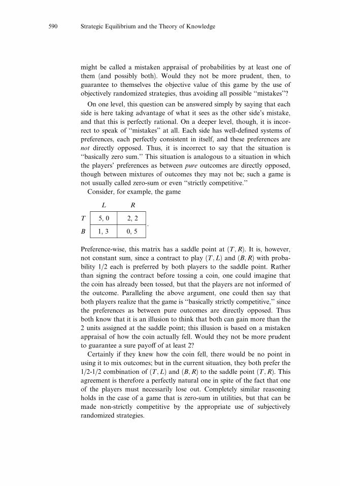
l. Another possible objection runs as follows: Both players realize that

the game is basically zero-sum, since in the last analysis, only one of them

can win the election. Both know it is an illusion to think that both can

gain more than the value of the game; this illusion is based on what


:

might be called a mistaken appraisal of probabilities by at least one of

them (and possibly both). Would they not be more prudent, then, to

guarantee to themselves the objective value of this game by the use of

objectively randomized strategies, thus avoiding all possible ‘‘mistakes’’?

On one level, this question can be answered simply by saying that each

side is here taking advantage of what it sees as the other side’s mistake,

and that this is perfectly rational. On a deeper level, though, it is incor-

rect to speak of ‘‘mistakes’’ at all. Each side has well-defined systems of

preferences, each perfectly consistent in itself, and these preferences are

not directly opposed. Thus, it is incorrect to say that the situation is

‘‘basically zero sum.’’ This situation is analogous to a situation in which

the players’ preferences as between pure outcomes are directly opposed,

though between mixtures of outcomes they may not be; such a game is

not usually called zero-sum or even ‘‘strictly competitive.’’

Consider, for example, the game

L R

T 5, 0 2, 2

B 1, 3 0, 5

Preference-wise, this matrix has a saddle point at (T ;R). It is, however,

not constant sum, since a contract to play (T ;L) and (B;R) with proba-

bility 1/2 each is preferred by both players to the saddle point. Rather

than signing the contract before tossing a coin, one could imagine that

the coin has already been tossed, but that the players are not informed of

the outcome. Paralleling the above argument, one could then say that

both players realize that the game is ‘‘basically strictly competitive,’’ since

the preferences as between pure outcomes are directly opposed. Thus

both know that it is an illusion to think that both can gain more than the

2 units assigned at the saddle point; this illusion is based on a mistaken

appraisal of how the coin actually fell. Would they not be more prudent

to guarantee a sure payo¤ of at least 2?

Certainly if they knew how the coin fell, there would be no point in

using it to mix outcomes; but in the current situation, they both prefer the

1/2-1/2 combination of (T ;L) and (B;R) to the saddle point (T ;R). This

agreement is therefore a perfectly natural one in spite of the fact that one

of the players must necessarily lose out. Completely similar reasoning

holds in the case of a game that is zero-sum in utilities, but that can be

made non-strictly competitive by the appropriate use of subjectively

randomized strategies.


Acknowledgement

Research supported in part by National Science Foundation grant GS-3269 at the Institutefor Mathematical Studies in the Social Sciences, Stanford University, and in part by CORE,the Center for Operations Research and Econometrics at the Catholic University ofLouvain.

References

Anscombe, F. J. and R. J. Aumann, 1963, A definition of subjective probability, Ann.Math. Stat. 34, 210–212 [Chapter 17].

Aumann, R. J., 1961, Almost strictly competitive games, J. Soc. Ind. Appl. Math. 9, 544–550 [Chapter 27].

Aumann, R. J., 1964, Mixed and behavior strategies in infinite extensive games, in:M. Dresher, L. S. Shapley and A. W. Tucker, eds., Advances in game theory (PrincetonUniversity Press, Princeton) 627–650 [Chapter 28].

Aumann, R. J. and M. Maschler, 1972, Some thoughts on the minimax principle, Manage-ment Science 18, P-54–P-63 [Chapter 29].

Harsanyi, J., 1967–68, Games of incomplete information played by Bayesian players, PartsI–III, Management Science 14, 159–182, 320–334, 486–502.

Harsanyi, J. and R. Selten, 1972, A generalized Nash solution for two-person bargaininggames with incomplete information, Management Science 18, P-80–P-106.

Kuhn, H. W., 1953, Extensive games and the problem of information, in: H. W. Kuhn andA. W. Tucker, eds., Contributions to the theory of games II (Princeton University Press,Princeton) 193–216.

Lyapunov, A., 1940, Sur les fonctions-vecteurs completement additives, Bull. Acad. Sci.USSR Ser. Math. 4, 465–478.

Nash, J. F., 1951, Non-cooperative games, Ann. of Math. 54, 286–295.

Savage, L. J., 1954, The foundations of statistics (John Wiley, New York).

Von Neumann, J. and O. Morgenstern, 1944, Theory of games and economic behavior(Princeton University Press, Princeton); 3rd ed., 1953.


1280-ch31 p 559. - ma.huji.ac.ilraumann/pdf/subjectivity and correlation.pdf · 31 subjectivity and...

Documents