13 an introduction to interacting simulated...
TRANSCRIPT
13
An Introduction to Interacting Simulated
Annealing
Juergen Gall, Bodo Rosenhahn, and Hans-Peter Seidel
Max-Planck Institute for Computer ScienceStuhlsatzenhausweg 85, 66123 Saarbrucken, Germany
Summary. Human motion capturing can be regarded as an optimization problemwhere one searches for the pose that minimizes a previously defined error functionbased on some image features. Most approaches for solving this problem use iterativemethods like gradient descent approaches. They work quite well as long as they donot get distracted by local optima. We introduce a novel approach for global opti-mization that is suitable for the tasks as they occur during human motion capturing.We call the method interacting simulated annealing since it is based on an inter-acting particle system that converges to the global optimum similar to simulatedannealing. We provide a detailed mathematical discussion that includes convergenceresults and annealing properties. Moreover, we give two examples that demonstratepossible applications of the algorithm, namely a global optimization problem anda multi-view human motion capturing task including segmentation, prediction, andprior knowledge. A quantative error analysis also indicates the performance and therobustness of the interacting simulated annealing algorithm.
13.1 Introduction
13.1.1 Motivation
Optimization problems arise in many applications of computer vision. In pose esti-mation, e.g. [28], and human motion capturing, e.g. [31], functions are minimized atvarious processing steps. For example, the marker-less motion capture system [26]minimizes in a first step an energy function for the segmentation. In a second step,correspondences between the segmented image and a 3D model are established. Theoptimal pose is then estimated by minimizing the error given by the correspondences.These optimization problems also occur, for instance, in model fitting [17, 31]. Theproblems are mostly solved by iterative methods as gradient descent approaches.The methods work very well as long as the starting point is near the global opti-mum, however, they get easily stuck in a local optimum. In order to deal with it,several random selected starting points are used and the best solution is selected inthe hope that at least one of them is near enough to the global optimum, cf. [26].Although it improves the results in many cases, it does not ensure that the globaloptimum is found.
320 J. Gall, B. Rosenhahn and H.-P. Seidel
In this chapter, we introduce a global optimization method based on an interactingparticle system that overcomes the dilemma of local optima and that is suitable forthe optimization problems as they arise in human motion capturing. In contrast tomany other optimization algorithms, a distribution instead of a single value is ap-proximated by a particle representation similar to particle filters [10]. This propertyis beneficial, particularly, for tracking where the right parameters are not alwaysexact at the global optimum depending on the image features that are used.
13.1.2 Related Work
A popular global optimization method inspired by statistical mechanics is known assimulated annealing [14, 18]. Similar to our approach, a function V ≥ 0 interpretedas energy is minimized by means of an unnormalized Boltzmann-Gibbs measure thatis defined in terms of V and an inverse temperature β > 0 by
g(dx) = exp (−β V (x)) λ(dx), (13.1)
where λ is the Lebesgue measure. This measure has the property that the probabilitymass concentrates at the global minimum of V as β →∞.The key idea behind simulated annealing is taking a random walk through thesearch space while β is successively increased. The probability of accepting a newvalue in the space is given by the Boltzmann-Gibbs distribution. While values withless energy than the current value are accepted with probability one, the probabilitythat values with higher energy are accepted decreases as β increases. Other relatedapproaches are fast simulated annealing [30] using a Cauchy-Lorentz distributionand generalized simulated annealing [32] based on Tsallis statistics.Interacting particle systems [19] approximate a distribution of interest by a finitenumber of weighted random variablesX(i) called particles. Provided that the weightsΠ(i) are normalized such that
PΠ(i) = 1, the set of weighted particles determines
a random probability measures by
nX
i=1
Π(i)δX(i) . (13.2)
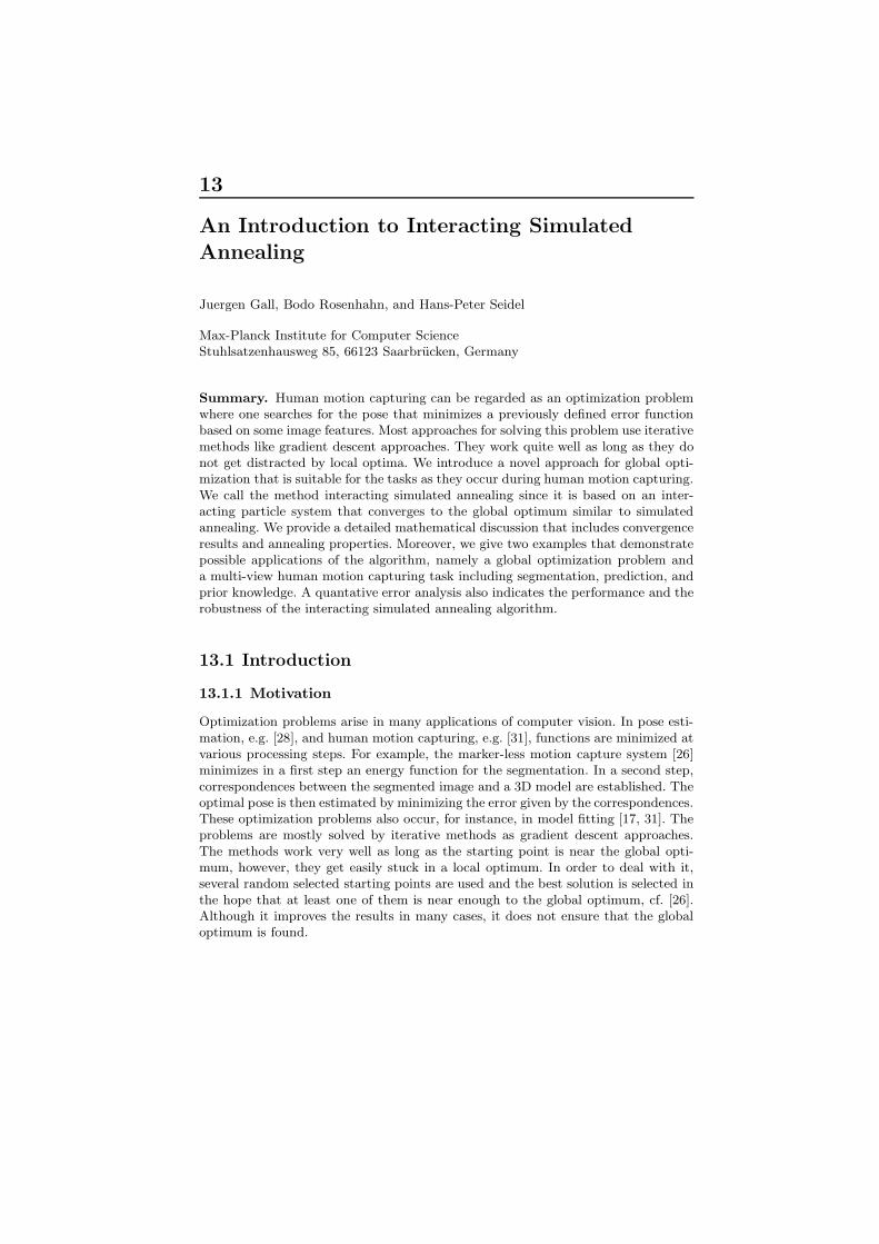
Depending on the weighting function and the distribution of the particles, the mea-sure converges to a distribution η as n tends to infinity. When the particles areidentically independently distributed according to η and uniformly weighted, i.e.Π(i) = 1/n, the convergence follows directly from the law of large numbers [3].Interacting particle systems are mostly known in computer vision as particle fil-ter [10] where they are applied for solving non-linear, non-Gaussian filtering prob-lems. However, these systems also apply for trapping analysis, evolutionary algo-rithms, statistics [19], and optimization as we demonstrate in this chapter. Theyusually consist of two steps as illustrated in Figure 13.1. During a selection step,the particles are weighted according to a weighting function and then resampledwith respect to their weights, where particles with a great weight generate moreoffspring than particles with lower weight. In a second step, the particles mutate orare diffused.
13 Interacting Simulated Annealing 321
Resampling:
particle
weighted particle
weighting functionWeighting:
Diffusion:
Fig. 13.1. Operation of an interacting particle system. After weighting the particles(black circles), the particles are resampled and diffused (gray circles).
13.1.3 Interaction and Annealing
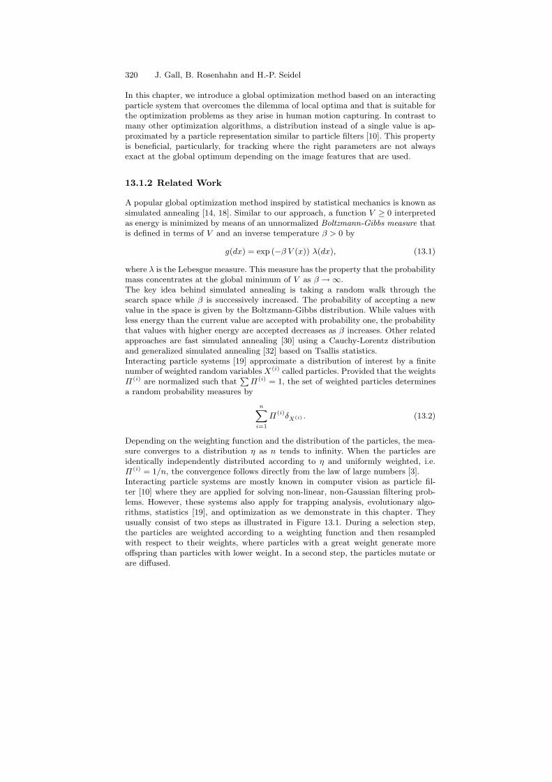
Simulated annealing approaches are designed for global optimization, i.e. for search-ing the global optimum in the entire search space. Since they are not capable offocusing the search on some regions of interest in dependency on the previous visitedvalues, they are not suitable for tasks in human motion capturing. Our approach,in contrast, is based on an interacting particle system that uses Boltzmann-Gibbsmeasures (13.1) similar to simulated annealing. This combination ensures not onlythe annealing property as we will show, but also exploits the distribution of the par-ticles in the space as measure for the uncertainty in an estimate. The latter allowsan automatic adaption of the search on regions of interest during the optimizationprocess. The principle of the annealing effect is illustrated in Figure 13.2.A first attempt to fuse interaction and annealing strategies for human motion cap-turing has become known as annealed particle filter [9]. Even though the heuristic isnot based on a mathematical background, it already indicates the potential of suchcombination. Indeed, the annealed particle filter can be regarded as a special caseof interacting simulated annealing where the particles are predicted for each frameby a stochastic process, see Section 13.3.1.
13.1.4 Outline
The interacting annealing algorithm is introduced in Section 13.3.1 and its asymp-totic behavior is discussed in Section 13.3.2. The given convergence results are basedon Feynman-Kac models [19] which are outlined in Section 13.2. Since a generaltreatment including proofs is out of the scope of this introduction, we refer the in-terested reader to [11] or [19]. While our approach is evaluated for a standard globaloptimization problem in Section 13.4.1, Section 13.4.2 demonstrates the performanceof interacting simulated annealing in a complete marker-less human motion capturesystem that includes segmentation, pose prediction and prior knowledge.

322 J. Gall, B. Rosenhahn and H.-P. Seidel
Fig. 13.2. Illustration of the annealing effect with three runs. Due to annealing,the particles migrate towards the global maximum without getting stuck in the localmaximum.
13.1.5 Notations
We always regard E as a subspace of Rd, and let B(E) denote its Borel σ-algebra.B(E) denotes the set of bounded measurable functions, δx is the Dirac measureconcentrated in x ∈ E, ‖ · ‖2 is the Euclidean norm, and ‖ · ‖∞ is the well-knownsupremum norm. Let f ∈ B(E), µ be a measure on E, and let K be a Markov kernelon E1. We write
〈µ, f〉 =
Z
E
f(x)µ(dx), 〈µ,K〉(B) =
Z
E
K(x,B)µ(dx) for B ∈ B(E).
Furthermore, U [0, 1] denotes the uniform distribution on the interval [0, 1] and
osc(ϕ) := supx,y∈E
|ϕ(x)− ϕ(y)| . (13.3)
is an upper bound for the oscillations of f .
13.2 Feynman-Kac Model
Let (Xt)t∈N0 be an E-valued Markov process with family of transition kernels(Kt)t∈N0 and initial distribution η0. We denote by Pη0 the distribution of the Markovprocess, i.e. for t ∈ N0,
Pη0 (d(x0, x1, . . . , xt)) = Kt−1(xt−1, dxt) . . . K0(x0, dx1) η0(dx0),
1 A Markov kernel is a function K : E × B(E) → [0,∞] such that K(·, B) isB(E)-measurable ∀B and K(x, ·) is a probability measure ∀x. An example of aMarkov kernel is given in Equation (13.12). For more details on probability theoryand Markov kernels, we refer to [3].

13 Interacting Simulated Annealing 323
and by Eη0 [·] the expectation with respect to Pη0 . The sequence of distributions(ηt)t∈N0 on E defined for any ϕ ∈ B(E) and t ∈ N0 as
〈ηt, ϕ〉 := 〈γt, ϕ〉〈γt, 1〉, 〈γt, ϕ〉 := Eη0
"ϕ (Xt) exp
−t−1X
s=0
βs V (Xs)
!#,
is called the Feynman-Kac model associated with the pair (exp(−βt V ), Kt).The Feynman-Kac model as defined above satisfies the recursion relation
ηt+1 = 〈Ψt(ηt), Kt〉, (13.4)
where the Boltzmann-Gibbs transformation Ψt is defined by
Ψt (ηt) (dyt) =Eη0
ˆexp
`−Pt−1
s=0 βs V (Xs)´˜
Eη0ˆexp
`−Pt
s=0 βs V (Xs)´˜ exp (−βt Vt(yt)) ηt(dyt).
The particle approximation of the flow (13.4) depends on a chosen family of Markovtransition kernels (Kt,ηt)t∈N0 satisfying the compatibility condition
〈Ψt (ηt) , Kt〉 := 〈ηt, Kt,ηt 〉.
A family (Kt,ηt)t∈N0 of kernels is not uniquely determined by these conditions.As in [19, Chapter 2.5.3], we choose
Kt,ηt = St,ηtKt, (13.5)
where
St,ηt (xt, dyt) = εt exp (−βt Vt(xt)) δxt(dyt)
+ (1 − εt exp (−βt Vt(xt))) Ψt (ηt) (dyt), (13.6)
with εt ≥ 0 and εt ‖exp(−βt V )‖∞ ≤ 1. The parameters εt may depend on thecurrent distribution ηt.
13.3 Interacting Simulated Annealing
Similar to simulated annealing, one can define an annealing scheme 0 ≤ β0 ≤ β1 ≤. . . ≤ βt in order to search for the global minimum of an energy function V . Undersome conditions that will be stated in Section 13.3.2, the flow of the Feynman-Kacdistribution becomes concentrated in the region of global minima of V as t goes toinfinity. Since it is not possible to sample from the distribution directly, the flow isapproximated by a particle set as it is done by a particle filter. We call the algorithmfor the flow approximation interacting simulated annealing (ISA).
13.3.1 Algorithm
The particle approximation for the Feynman-Kac model is completely describedby the Equation (13.5). The particle system is initialized by n identically, inde-
pendently distributed random variables X(i)0 with common law η0 determining the
324 J. Gall, B. Rosenhahn and H.-P. Seidel
random probability measure ηn0 :=Pni=1 δX(i)
0
/n. Since Kt,ηt can be regarded as
the composition of a pair of selection and mutation Markov kernels, we split thetransitions into the following two steps
ηntSelection−−−−−−−−→ ηnt
Mutation−−−−−−−−→ ηnt+1,
where
ηnt :=1
n
nX
i=1
δX
(i)t
, ηnt :=1
n
nX
i=1
δX
(i)t
.
During the selection step each particle X(i)t evolves according to the Markov tran-
sition kernel St,ηnt(X
(i)t , ·). That means X
(i)t is accepted with probability
εt exp(−βt V (X(i)t )), (13.7)
and we set X(i)t = X
(i)t . Otherwise, X
(i)t is randomly selected with distribution
nX
i=1
exp(−βt V (X(i)t ))
Pnj=1 exp(−βt V (X
(j)t ))
δX
(i)t
.
The mutation step consists in letting each selected particle X(i)t evolve according to
the Markov transition kernel Kt(X(i)t , ·).
Algorithm 6 Interacting Simulated Annealing Algorithm
Requires: parameters (εt)t∈N0 , number of particles n, initial distribution η0, energyfunction V , annealing scheme (βt)t∈N0 and transitions (Kt)t∈N0
1. Initialization• Sample x
(i)0 from η0 for all i
2. Selection• Set π(i) ← exp(−βt V (x
(i)t )) for all i
• For i from 1 to n:Sample κ from U [0, 1]If κ ≤ εtπ(i) then? Set x
(i)t ← x
(i)t
Else? Set x
(i)t ← x
(j)t with probability π(j)
Pnk=1
π(k)
3. Mutation• Sample x
(i)t+1 from Kt(x
(i)t , ·) for all i and go to step 2
There are several ways to choose the parameter εt of the selection kernel (13.6) thatdefines the resampling procedure of the algorithm, cf. [19]. If
εt := 0 ∀t, (13.8)
the selection can be done by multinomial resampling. Provided that2
2 The inequality satisfies the condition εt ‖exp(−βt V )‖∞ ≤ 1 for Equation (13.6).
13 Interacting Simulated Annealing 325
n ≥ supt
(exp(βt osc(V )) ,
another selection kernel is given by
εt(ηt) :=1
n 〈ηt, exp(−βt V )〉 . (13.9)
In this case the expression εtπ(i) in Algorithm 6 is replaced by π(i)/
Pnk=1 π
(k). Athird kernel is determined by
εt(ηt) :=1
inf y ∈ R : ηt (x ∈ E : exp(−βt V (x)) > y) = 0 , (13.10)
yielding the expression π(i)/max1≤k≤n π(k) instead of εtπ
(i).Pierre del Moral showed in [19, Chapter 9.4] that for any t ∈ N0 and ϕ ∈ B(E) thesequence of random variables
√n(〈ηnt , ϕ〉 − 〈ηt, ϕ〉)
converges in law to a Gaussian random variable W when the selection kernel (13.6)is used to approximate the flow (13.4). Moreover, it turns out that when (13.9) ischosen, the variance of W is strictly smaller than in the case with εt = 0.We remark that the annealed particle filter [9] relies on interacting simulated an-nealing with εt = 0. The operation of the method is illustrated by
ηntPrediction−−−−−−−−→ ηnt+1
ISA−−−−−−−−→ ηnt+1.
The ISA is initialized by the predicted particles X(i)t+1 and performs M times the
selection and mutation steps. Afterwards the particles X(i)t+1 are obtained by an
additional selection. This shows that the annealed particle filter uses a simulatedannealing principle to locate the global minimum of a function V at each time step.
13.3.2 Convergence
This section discusses the asymptotic behavior of the interacting simulated annealingalgorithm. For this purpose, we introduce some definitions in accordance with [19]and [15].
Definition 1. A kernel K on E is called mixing if there exists a constant 0 < ε < 1such that
K(x1, ·) ≥ εK(x2, ·) ∀x1, x2 ∈ E. (13.11)
The condition can typically only be established when E ⊂ Rd is a bounded subset,
which is the case in many applications like human motion capturing. For examplethe (bounded) Gaussian distribution on E
K(x,B) :=1
Z
Z
B
exp
„−1
2(x− y)T Σ−1 (x− y)
«dy, (13.12)
where Z :=RE
exp(− 12
(x−y)T Σ−1 (x−y)) dy, is mixing if and only if E is bounded.Moreover, a Gaussian with a high variance satisfies the mixing condition with alarger ε than a Gaussian with lower variance.
326 J. Gall, B. Rosenhahn and H.-P. Seidel
Definition 2. The Dobrushin contraction coefficient of a kernel K on E is definedby
β(K) := supx1,x2∈E
supB∈B(E)
|K(x1, B)−K(x2, B)| . (13.13)
Furthermore, β(K) ∈ [0, 1] and β(K1K2) ≤ β(K1) β(K2).
When the kernel M is a composition of several mixing Markov kernels, i.e. M :=KsKs+1 . . . Kt, and each kernel Kk satisfies the mixing condition for some εk, theDobrushin contraction coefficient can be estimated by β(M) ≤ Qt
k=s(1− εk).The asymptotic behavior of the interacting simulated annealing algorithm is affectedby the convergence of the flow of the Feynman-Kac distribution (13.4) to the regionof global minima of V as t tends to infinity and by the convergence of the particleapproximation to the Feynman-Kac distribution at each time step t as the numberof particles n tends to infinity.
Convergence of the flow
We suppose that Kt = K is a Markov kernel satisfying the mixing condition (13.11)for an ε ∈ (0, 1) and osc(V ) <∞. A time mesh is defined by
t(n) := n(1 + bc(ε)c) c(ε) := (1− ln(ε/2))/ε2 for n ∈ N0. (13.14)
Let 0 ≤ β0 ≤ β1 . . . be an annealing scheme such that βt = βt(n+1) is constant in theinterval (t(n), t(n+1)]. Furthermore, we denote by ηt the Feynman-Kac distributionafter the selection step, i.e. ηt = Ψt(ηt). According to [19, Proposition 6.3.2], we have
Theorem 1. Let b ∈ (0, 1) and βt(n+1) = (n + 1)b. Then for each δ > 0
limn→∞
ηt(n) (V ≥ V? + δ) = 0,
where V? = supv ≥ 0; V ≥ v a.e..The rate of convergence is d/n(1−b) where d is increasing with respect to b and c(ε)but does not depend on n as given in [19, Theorem 6.3.1]. This theorem establishesthat the flow of the Feynman-Kac distribution ηt becomes concentrated in the regionof global minima as t→ +∞.
Convergence of the particle approximation
Del Moral established the following convergence theorem [19, Theorem 7.4.4].
Theorem 2. For any ϕ ∈ B(E),
Eη0 [|〈ηnt+1, ϕ〉 − 〈ηt+1, ϕ〉|] ≤ 2 osc(ϕ)√n
1 +
tX
s=0
rsβ(Ms)
!,
where
rs := exp
osc(V )
tX
r=s
βr
!,
Ms := KsKs+1 . . . Kt,
for 0 ≤ s ≤ t.
13 Interacting Simulated Annealing 327
Assuming that the kernels Ks satisfy the mixing condition with εs, we get a roughestimate for the number of particles
n ≥ 4 osc(ϕ)2
δ2
1 +
tX
s=0
(exp
osc(V )
tX
r=s
βr
!tY
k=s
(1 − εk))!2
(13.15)
needed to achieve a mean error less than a given δ > 0.
Optimal transition kernel
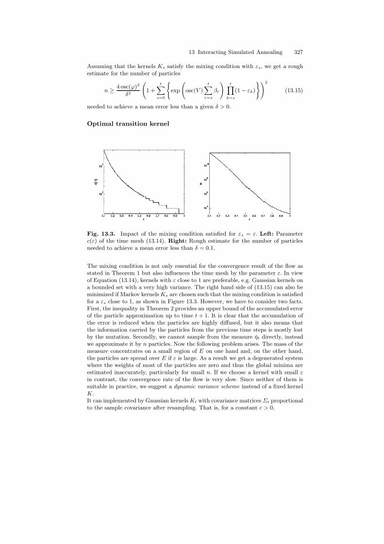
Fig. 13.3. Impact of the mixing condition satisfied for εs = ε. Left: Parameterc(ε) of the time mesh (13.14). Right: Rough estimate for the number of particlesneeded to achieve a mean error less than δ = 0.1.
The mixing condition is not only essential for the convergence result of the flow asstated in Theorem 1 but also influences the time mesh by the parameter ε. In viewof Equation (13.14), kernels with ε close to 1 are preferable, e.g. Gaussian kernels ona bounded set with a very high variance. The right hand side of (13.15) can also beminimized if Markov kernelsKs are chosen such that the mixing condition is satisfiedfor a εs close to 1, as shown in Figure 13.3. However, we have to consider two facts.First, the inequality in Theorem 2 provides an upper bound of the accumulated errorof the particle approximation up to time t + 1. It is clear that the accumulation ofthe error is reduced when the particles are highly diffused, but it also means thatthe information carried by the particles from the previous time steps is mostly lostby the mutation. Secondly, we cannot sample from the measure ηt directly, insteadwe approximate it by n particles. Now the following problem arises. The mass of themeasure concentrates on a small region of E on one hand and, on the other hand,the particles are spread over E if ε is large. As a result we get a degenerated systemwhere the weights of most of the particles are zero and thus the global minima areestimated inaccurately, particularly for small n. If we choose a kernel with small εin contrast, the convergence rate of the flow is very slow. Since neither of them issuitable in practice, we suggest a dynamic variance scheme instead of a fixed kernelK.It can implemented by Gaussian kernelsKt with covariance matrices Σt proportionalto the sample covariance after resampling. That is, for a constant c > 0,
328 J. Gall, B. Rosenhahn and H.-P. Seidel
Σt :=c
n− 1
nX
i=1
(x(i)t − µt)ρ (x
(i)t − µt)Tρ , µt :=
1
n
nX
i=1
x(i)t , (13.16)
where ((x)ρ)k = max(xk, ρ) for a ρ > 0. The value ρ ensures that the variance doesnot become zero. The elements off the diagonal are usually set to zero, in order toreduce computation time.
Optimal parameters
The computation cost of the interacting simulated annealing algorithm with n par-ticles and T annealing runs is O(nT ), where
nT := n · T . (13.17)
While more particles give a better particle approximation of the Feynman-Kac dis-tribution, the flow becomes more concentrated in the region of global minima asthe number of annealing runs increases. Therefore, finding the optimal values is atrade-off between the convergence of the flow and the convergence of the particleapproximation provided that nT is fixed.Another important parameter of the algorithm is the annealing scheme. The schemegiven in Theorem 1 ensures convergence for any energy function V — even for theworst one in the sense of optimization — as long as osc(V ) <∞ but is too slow formost applications, as it is the case for simulated annealing. In our experiments theschemes
βt = ln(t+ b) for some b > 1 (logarithmic), (13.18)
βt = (t+ 1)b for some b ∈ (0, 1) (polynomial) (13.19)
performed well. Note that in contrast to the time mesh (13.14) the schemes are notanymore constant on a time interval.Even though a complete evaluation of the various parameters is out of the scope ofthis introduction, the examples given in the following section demonstrate settingsthat perform well, in particular for human motion capturing.
13.4 Examples
13.4.1 Global Optimization
The Ackley function [2, 1]
f(x) = −20 exp
0@−0.2
vuut1
d
dX
i=1
x2i
1A − exp
1
d
dX
i=1
cos(2π xi)
!+ 20 + e
is a widely used multimodal test function for global optimization algorithms. Asone can see from Figure 13.4, the function has a global minimum at (0, 0) thatis surrounded by several local minima. The problem consists of finding the global
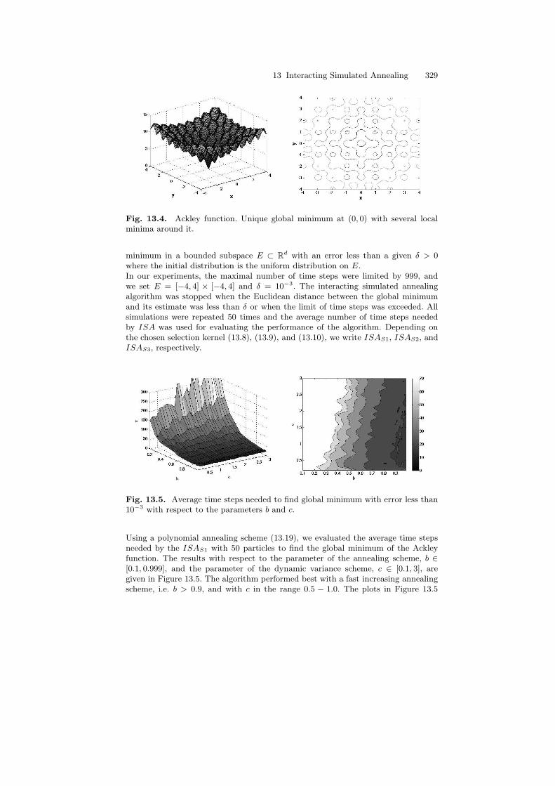
13 Interacting Simulated Annealing 329
Fig. 13.4. Ackley function. Unique global minimum at (0, 0) with several localminima around it.
minimum in a bounded subspace E ⊂ Rd with an error less than a given δ > 0
where the initial distribution is the uniform distribution on E.In our experiments, the maximal number of time steps were limited by 999, andwe set E = [−4, 4] × [−4, 4] and δ = 10−3. The interacting simulated annealingalgorithm was stopped when the Euclidean distance between the global minimumand its estimate was less than δ or when the limit of time steps was exceeded. Allsimulations were repeated 50 times and the average number of time steps neededby ISA was used for evaluating the performance of the algorithm. Depending onthe chosen selection kernel (13.8), (13.9), and (13.10), we write ISAS1, ISAS2, andISAS3, respectively.
Fig. 13.5. Average time steps needed to find global minimum with error less than10−3 with respect to the parameters b and c.
Using a polynomial annealing scheme (13.19), we evaluated the average time stepsneeded by the ISAS1 with 50 particles to find the global minimum of the Ackleyfunction. The results with respect to the parameter of the annealing scheme, b ∈[0.1, 0.999], and the parameter of the dynamic variance scheme, c ∈ [0.1, 3], aregiven in Figure 13.5. The algorithm performed best with a fast increasing annealingscheme, i.e. b > 0.9, and with c in the range 0.5 − 1.0. The plots in Figure 13.5

330 J. Gall, B. Rosenhahn and H.-P. Seidel
also reveal that the annealing scheme has greater impact on the performance thanthe factor c. When the annealing scheme increases slowly, i.e. b < 0.2, the globalminimum was actually not located within the given limit for all 50 simulations.
Ackley Ackley with noise
ISAS1 ISAS2 ISAS3 ISAS1 ISAS2 ISAS3
b 0.993 0.987 0.984 0.25 0.35 0.27
c 0.8 0.7 0.7 0.7 0.7 0.9
t 14.34 15.14 14.58 7.36 7.54 7.5
Table 13.1. Parameters b and c with lowest average time t for different selectionkernels.
The best results with parameters b and c for ISAS1, ISAS2, and ISAS3 are listed inTable 13.1. The optimal parameters for the three selection kernels are quite similarand the differences of the average time steps are marginal.
Fig. 13.6. Left: Average time steps needed to find global minimum with respectto number of particles. Right: Computation cost.
In a second experiment, we fixed the parameters b and c, where we used the valuesfrom Table 13.1, and varied the number of particles in the range 4 − 200 with stepsize 2. The results for ISAS1 are shown in Figure 13.6. While the average of timesteps declines rapidly for n ≤ 20, it is hardly reduced for n ≥ 40. Hence, nt and thusthe computation cost are lowest in the range 20 − 40. This shows that a minimumnumber of particles are required to achieve a success rate of 100%, i.e., the limitwas not exceeded for all simulations. In this example, the success rate was 100%for n ≥ 10. Furthermore, it indicates that the average of time steps is significantlyhigher for n less than the optimal number of particles. The results for ISAS1, ISAS2,and ISAS3 are quite similar. The best results are listed in Table 13.2.The ability of dealing with noisy energy functions is one of the strength of ISAas we will demonstrate. This property is very usefull for applications where themeasurement of the energy of a particle is distorted by noise. On the left hand side
13 Interacting Simulated Annealing 331
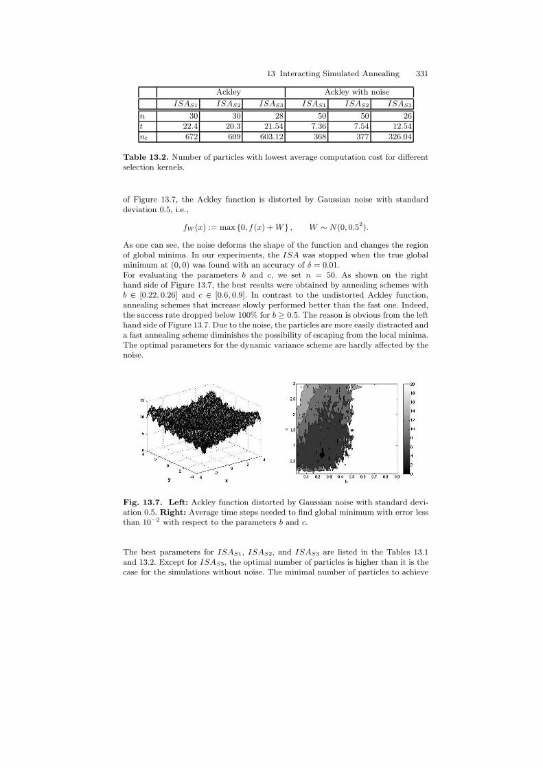
Ackley Ackley with noise
ISAS1 ISAS2 ISAS3 ISAS1 ISAS2 ISAS3
n 30 30 28 50 50 26
t 22.4 20.3 21.54 7.36 7.54 12.54
nt 672 609 603.12 368 377 326.04
Table 13.2. Number of particles with lowest average computation cost for differentselection kernels.
of Figure 13.7, the Ackley function is distorted by Gaussian noise with standarddeviation 0.5, i.e.,
fW (x) := max 0, f(x) +W , W ∼ N(0, 0.52).
As one can see, the noise deforms the shape of the function and changes the regionof global minima. In our experiments, the ISA was stopped when the true globalminimum at (0, 0) was found with an accuracy of δ = 0.01.For evaluating the parameters b and c, we set n = 50. As shown on the righthand side of Figure 13.7, the best results were obtained by annealing schemes withb ∈ [0.22, 0.26] and c ∈ [0.6, 0.9]. In contrast to the undistorted Ackley function,annealing schemes that increase slowly performed better than the fast one. Indeed,the success rate dropped below 100% for b ≥ 0.5. The reason is obvious from the lefthand side of Figure 13.7. Due to the noise, the particles are more easily distracted anda fast annealing scheme diminishes the possibility of escaping from the local minima.The optimal parameters for the dynamic variance scheme are hardly affected by thenoise.
Fig. 13.7. Left: Ackley function distorted by Gaussian noise with standard devi-ation 0.5. Right: Average time steps needed to find global minimum with error lessthan 10−2 with respect to the parameters b and c.
The best parameters for ISAS1, ISAS2, and ISAS3 are listed in the Tables 13.1and 13.2. Except for ISAS3, the optimal number of particles is higher than it is thecase for the simulations without noise. The minimal number of particles to achieve

332 J. Gall, B. Rosenhahn and H.-P. Seidel
a success rate of 100% also increased, e.g. 28 for ISAS1. We remark that ISAS3
required the least number of particles for a complete success rate, namely 4 for theundistorted energy function and 22 in the noisy case.We finish this section by illustrating two examples of energy function where the dy-namic variance schemes might not be suitable. On the left hand side of Figure 13.8,an energy function with shape similar to the Ackley function is drawn. The dynamicvariance schemes perform well for this type of function with an unique global mini-mum with several local minima around it. Due to the scheme, the search focuses onthe region near the global minimum after some time steps. The second function, seeFigure 8(b), has several, widely separated global minima yielding a high varianceof the particles even in the case that the particles are near to the global minima.Moreover, when the region of global minima is regarded as a sum of Dirac measures,the mean is not essentially a global minimum. In the last example shown on theright hand side of Figure 13.8, the global minimum is a small peak far away froma broad basin with a local minimum. When all particles fall into the basin, the dy-namic variance schemes focus the search on the region near the local minimum andit takes a long time to discover the global minimum.
(a) (b) (c)
Fig. 13.8. Different cases of energy functions. (a) Optimal for dynamic varianceschemes. An unique global minimum with several local minima around it. (b) Severalglobal minima that are widely separated. This yields a high variance even in the casethat the particles are near to the global minima. (c) The global minimum is a smallpeak far away from a broad basin. When all particles fall into the basin, the dynamicvariance schemes focus the search on the basin.
In most optimization problems arising in the field of computer vision, however, thefirst case occurs where the dynamic variance schemes perform well. One applicationis human motion capturing which we will discuss in the next section.
13.4.2 Human Motion Capture
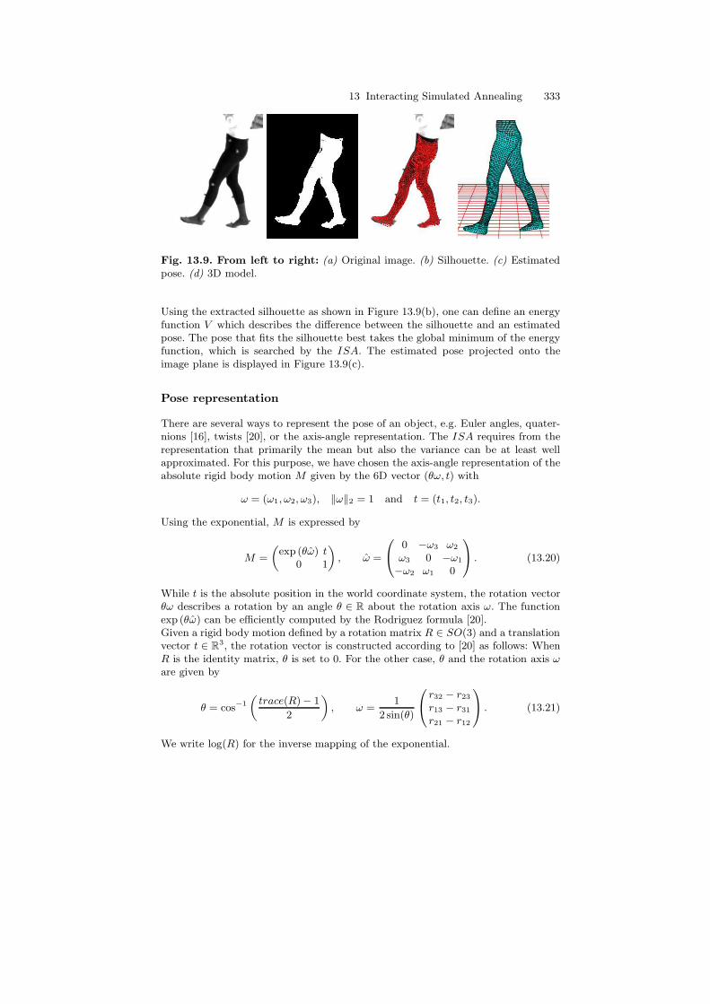
In our second experiment, we apply the interacting simulated annealing algorithmto model-based 3D tracking of the lower part of a human body, see Figure 13.9(a).This means that the 3D rigid body motion (RBM) and the joint angles, also calledthe pose, are estimated by exploiting the known 3D model of the tracked object. Themesh model illustrated in Figure 13.9(d) has 18 degrees of freedom (DoF), namely6 for the rigid body motion and 12 for the joint angles of the hip, knees, and feet.Although a marker-less motion capture system is discussed, markers are also stickedto the target object in order to provide a quantitative comparison with a commercialmarker based system.
13 Interacting Simulated Annealing 333
Fig. 13.9. From left to right: (a) Original image. (b) Silhouette. (c) Estimatedpose. (d) 3D model.
Using the extracted silhouette as shown in Figure 13.9(b), one can define an energyfunction V which describes the difference between the silhouette and an estimatedpose. The pose that fits the silhouette best takes the global minimum of the energyfunction, which is searched by the ISA. The estimated pose projected onto theimage plane is displayed in Figure 13.9(c).
Pose representation
There are several ways to represent the pose of an object, e.g. Euler angles, quater-nions [16], twists [20], or the axis-angle representation. The ISA requires from therepresentation that primarily the mean but also the variance can be at least wellapproximated. For this purpose, we have chosen the axis-angle representation of theabsolute rigid body motion M given by the 6D vector (θω, t) with
ω = (ω1, ω2, ω3), ‖ω‖2 = 1 and t = (t1, t2, t3).
Using the exponential, M is expressed by
M =
„exp (θω) t
0 1
«, ω =
0@
0 −ω3 ω2
ω3 0 −ω1
−ω2 ω1 0
1A . (13.20)
While t is the absolute position in the world coordinate system, the rotation vectorθω describes a rotation by an angle θ ∈ R about the rotation axis ω. The functionexp (θω) can be efficiently computed by the Rodriguez formula [20].Given a rigid body motion defined by a rotation matrix R ∈ SO(3) and a translationvector t ∈ R
3, the rotation vector is constructed according to [20] as follows: WhenR is the identity matrix, θ is set to 0. For the other case, θ and the rotation axis ωare given by
θ = cos−1
„trace(R)− 1
2
«, ω =
1
2 sin(θ)
0@r32 − r23r13 − r31r21 − r12
1A . (13.21)
We write log(R) for the inverse mapping of the exponential.
334 J. Gall, B. Rosenhahn and H.-P. Seidel
The mean of a set of rotations ri in the axis-angle representation can be computedby using the exponential and the logarithm as described in [22, 23]. The idea is tofind a geodesic on the Riemannian manifold determined by the set of 3D rotations.When the geodesic starting from the mean rotation in the manifold is mapped bythe logarithm onto the tangent space at the mean, it is a straight line starting atthe origin. The tangent space is called exponential chart .Hence, using the notations
r2 ? r1 = log (exp(r2) · exp(r1)) , r−11 = log
“exp(r1)
T”
for the rotation vectors r1 and r2, the mean rotation r satisfies
X
i
`r−1 ? ri
´= 0. (13.22)
Weighting each rotation with πi, yields the least squares problem:
1
2
X
i
πi‚‚r−1 ? ri
‚‚2
2→ min. (13.23)
The weighted mean can thus be estimated by
rt+1 = rt ?
Pi πi
`r−1t ? ri
´Pi πi
!. (13.24)
The gradient descent method takes about 5 iterations until it converges.The variance and the normal density on a Riemannian manifold can also be approxi-mated, cf. [24]. Since, however, the variance is only used for diffusing the particles, avery accurate approximation is not needed. Hence, the variance of a set of rotationsri is calculated in the Euclidean space R
3.The twist representation used in [7, 26] and in chapters 11 and 12 is quite similar.Instead of a separation between the translation t and the rotation r, it describesa screw motion where the motion velocity θ also affects the translation. A twistξ ∈ se(3)3 is represented by
θξ = θ
„ω v0 0
«, (13.25)
where exp(θξ) is a rigid body motion.The logarithm of a rigid body motion M ∈ SE(3) is the following transformation:
θω = log(R), v = A−1t, (13.26)
whereA = (I − exp(θω))ω + ωωT θ (13.27)
is obtained from the Rodriguez formula. This follows from the fact, that the twomatrices which comprise A have mutually orthogonal null spaces when θ 6= 0. Hence,Av = 0⇔ v = 0.We remark that the two representations are identical for the joints where only a ro-tation around a known axis is performed. Furthermore, a linearization is not neededfor the ISA in contrast to the pose estimation as described in chapters 11 and 12
3 se(3) is the Lie algebra that corresponds to the Lie group SE(3).
13 Interacting Simulated Annealing 335
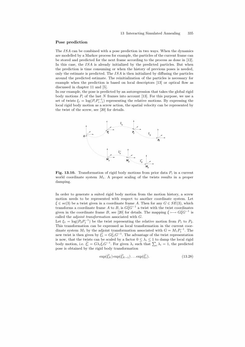
Pose prediction
The ISA can be combined with a pose prediction in two ways. When the dynamicsare modelled by a Markov process for example, the particles of the current frame canbe stored and predicted for the next frame according to the process as done in [12].In this case, the ISA is already initialized by the predicted particles. But whenthe prediction is time consuming or when the history of previous poses is needed,only the estimate is predicted. The ISA is then initialized by diffusing the particlesaround the predicted estimate. The reinitialization of the particles is necessary forexample when the prediction is based on local descriptors [13] or optical flow asdiscussed in chapter 11 and [5].In our example, the pose is predicted by an autoregression that takes the global rigidbody motions Pi of the last N frames into account [13]. For this purpose, we use aset of twists ξi = log(PiP
−1i−1) representing the relative motions. By expressing the
local rigid body motion as a screw action, the spatial velocity can be represented bythe twist of the screw, see [20] for details.
M
P P
P3
M
ξ
ξ’
O1
ξ1
22
1
1 2 ξ2’
M3
Fig. 13.10. Transformation of rigid body motions from prior data Pi in a currentworld coordinate system M1. A proper scaling of the twists results in a properdamping.
In order to generate a suited rigid body motion from the motion history, a screwmotion needs to be represented with respect to another coordinate system. Letξ ∈ se(3) be a twist given in a coordinate frame A. Then for any G ∈ SE(3), whichtransforms a coordinate frame A to B, is GξG−1 a twist with the twist coordinatesgiven in the coordinate frame B, see [20] for details. The mapping ξ 7−→ GξG−1 iscalled the adjoint transformation associated with G.Let ξ1 = log(P2P
−11 ) be the twist representing the relative motion from P1 to P2.
This transformation can be expressed as local transformation in the current coor-dinate system M1 by the adjoint transformation associated with G = M1P
−11 . The
new twist is then given by ξ′1 = Gξ1G−1. The advantage of the twist representation
is now, that the twists can be scaled by a factor 0 ≤ λi ≤ 1 to damp the local rigidbody motion, i.e. ξ′i = GλiξiG
−1. For given λi such thatPi λi = 1, the predicted
pose is obtained by the rigid body transformation
exp(ξ′N ) exp(ξ′N−1) . . . exp(ξ′1). (13.28)

336 J. Gall, B. Rosenhahn and H.-P. Seidel
Energy function
The energy function V of a particle x, which is used for our example, depends onthe extracted silhouette and on some learned prior knowledge as in [12], but it isdefined in a different way.Silhouette: First of all, the silhouette is extracted from an image by a level setbased segmentation as in [8, 27]. We state the energy functional E for convenienceonly and refer the reader to chapter 11 where the segmentation is described in detail.Let Ωi be the image domain of view i and let Φi0(bx ) be the contour of the predictedpose in Ωi. In order to obtain the silhouettes for all r views, the energy functionalE(bx, Φ1, . . . , Φr) =
Pri=1 E(bx, Φi) is minimzed, where
E(bx, Φi) = −ZH(Φi) ln pi1 + (1−H(Φi)) ln pi2 dx
+ ν
Z
Ωi
˛˛∇H(Φi)
˛˛ dx+ λ
Z
Ωi
“Φi − Φi0(bx )
”2
dx. (13.29)
In our experiments, we weighted the smoothness term with ν = 4 and the shapeprior with λ = 0.04.After the segmentation, 3D-2D correspondences between the 3D model (Xi) and a2D image (xi) are established by the projected vertices of the 3D mesh that arepart of the model contour and their closest points of the extracted contour thatare determined by a combination of an iterated closest point algorithm [4] and anoptic flow based shape registration [25]. More details about the shape matching aregiven in chapter 12. We write each correspondence as pair (Xi, xi) of homogeneouscoordinates.Each image point xi defines a projection ray that can be represented as Pluckerline [20] determined by a unique vector ni and a momentmi such that x×ni−mi = 0for all x on the 3D line. Furthermore,
‖x× ni −mi‖2 (13.30)
is the norm of the perpendicular error vector between the line and a point x ∈ R3.
As we already mentioned, a joint j is represented by the rotation angle θj . Hence,we write M(ω, t) for the rigid body motion and M(θj) for the joints. Furthermore,we have to consider the kinematic chain of articulated objects. Let Xi be a point onthe limb ki whose position is influenced by si joints in a certain order. The inverseorder of these joints is then given by the mapping ιki
, e.g., a point on the left shankis influenced by the left knee joint ιki
(4) and by the three joints of the left hip ιki(3),
ιki(2), and ιki
(1).Hence, the pose estimation consists of finding a pose x such that the error
errS(x, i) :=
‚‚‚‚“M(ω, t)M(θιki
(1)) . . .M(θιki(si))Xi
”3×1× ni −mi
‚‚‚‚2
(13.31)
is minimal for all pairs, where (·)3×1 denotes the transformation from homogeneouscoordinates back to non-homogeneous coordinates.Prior Knowledge: Using prior knowledge about the probability of a certain posecan stabilize the pose estimation as shown in [12] and [6]. The prior ensures thatparticles representing a familiar pose are favored in problematic situations, e.g.,when the observed object is partially occluded. As discussed in chapter 11, the

13 Interacting Simulated Annealing 337
probability of the various poses is learned from N training samples, where the densityis estimated by a Parzen-Rosenblatt estimator [21, 29] with a Gaussian kernel
ppose(x) =1
(2 π σ2)d/2N
NX
i=1
exp
„−‖xi − x‖
22
2σ2
«. (13.32)
In our experiments, we chose the window size σ as the maximum second nearestneighbor distance between all training samples as in [12].Incorporating the learned probability of the poses in the energy function has addi-tional advantages. First, it already incorporates correlations between the parametersof a pose – and thus of a particle – yielding an energy function that is closer to themodel and the observed object. Moreover, it can be regarded as a soft constraint thatincludes anatomical constraints, e.g. by the limited freedom of joints movement, andthat prevents the estimates from self-intersections since unrealistic and impossibleposes cannot be contained in the training data.Altogether, the energy function V of a particle x is defined by
V (x) :=1
l
lX
i=1
errS(x, i)2 − η ln(ppose(x)), (13.33)
where l is the number of correspondences. In our experiments, we set η = 8.
Results
Fig. 13.11. Left: Results for a walking sequence captured by four cameras (200frames). Right: The joint angles of the right and left knee in comparison with amarker based system.
In our experiments, we tracked the lower part of a human body using four calibratedand synchronized cameras. The walking sequence was simultaneously captured by acommercial marker based system4 allowing a quantitative error analysis. The train-ing data used for learning ppose consisted of 480 samples that were obtained fromwalking sequences. The data was captured by the commercial system before record-ing the test sequence that was not contained in the training data.
4 Motion Analysis system with 8 Falcon cameras.
338 J. Gall, B. Rosenhahn and H.-P. Seidel
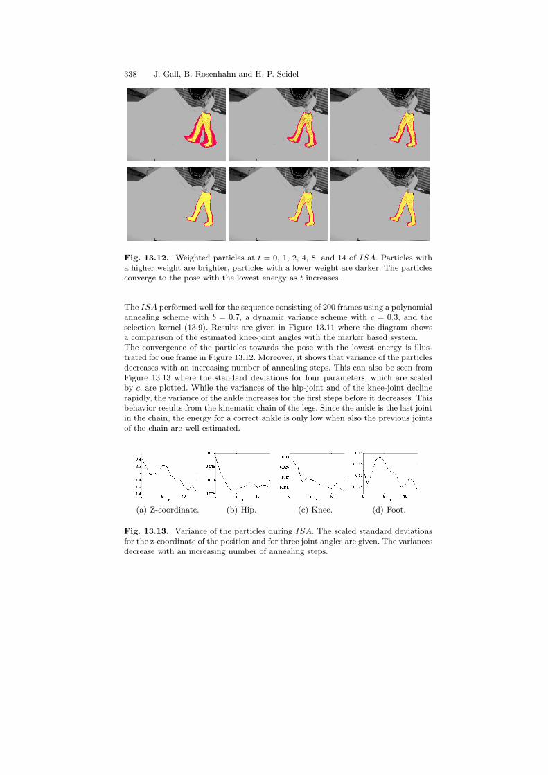
Fig. 13.12. Weighted particles at t = 0, 1, 2, 4, 8, and 14 of ISA. Particles witha higher weight are brighter, particles with a lower weight are darker. The particlesconverge to the pose with the lowest energy as t increases.
The ISA performed well for the sequence consisting of 200 frames using a polynomialannealing scheme with b = 0.7, a dynamic variance scheme with c = 0.3, and theselection kernel (13.9). Results are given in Figure 13.11 where the diagram showsa comparison of the estimated knee-joint angles with the marker based system.The convergence of the particles towards the pose with the lowest energy is illus-trated for one frame in Figure 13.12. Moreover, it shows that variance of the particlesdecreases with an increasing number of annealing steps. This can also be seen fromFigure 13.13 where the standard deviations for four parameters, which are scaledby c, are plotted. While the variances of the hip-joint and of the knee-joint declinerapidly, the variance of the ankle increases for the first steps before it decreases. Thisbehavior results from the kinematic chain of the legs. Since the ankle is the last jointin the chain, the energy for a correct ankle is only low when also the previous jointsof the chain are well estimated.
(a) Z-coordinate. (b) Hip. (c) Knee. (d) Foot.
Fig. 13.13. Variance of the particles during ISA. The scaled standard deviationsfor the z-coordinate of the position and for three joint angles are given. The variancesdecrease with an increasing number of annealing steps.

13 Interacting Simulated Annealing 339
Fig. 13.14. Left: Energy of estimate for walking sequence (200 frames). Right:Error of estimate (left and right knee).
On the right hand side of Figure 13.14, the energy of the estimate during trackingis plotted. We also plotted the root-mean-square error of the estimated knee-anglesfor comparison where we used the results from the marker based system as groundtruth with an accuracy of 3 degrees. For n = 250 and T = 15, we achieved an overallroot-mean-square error of 2.74 degrees. The error was still below 3 degrees with 375particles and T = 7, i.e. nT = 2625. With this setting, the ISA took 7−8 seconds forapproximately 3900 correspondences that were established in the 4 images of oneframe. The whole system including segmentation, took 61 seconds for one frame.For comparison, the iterative method as used in chapter 12 took 59 seconds with anerror of 2.4 degrees. However, we have to remark that for this sequence the iterativemethod performed very well. This becomes clear from the fact that no additionalrandom starting points were needed. Nevertheless, it demonstrates that the ISAcan keep up even in situations that are perfect for iterative methods.
Fig. 13.15. Left: Random pixel noise. Right: Occlusions by random rectangles.
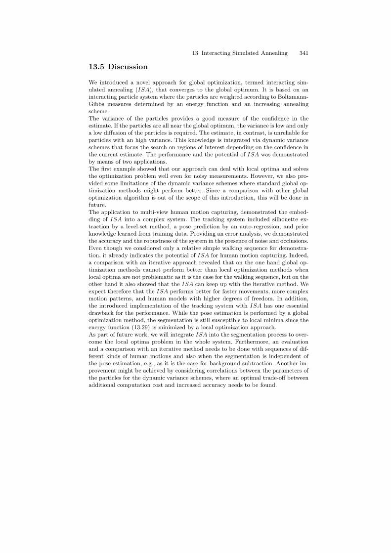
Figures 13.16 and 13.17 show the robustness in the presence of noise and occlusions.For the first sequence, each frame was independently distorted by 70% pixel noise,i.e., each pixel value was replaced with probability 0.7 by a value uniformly sampled
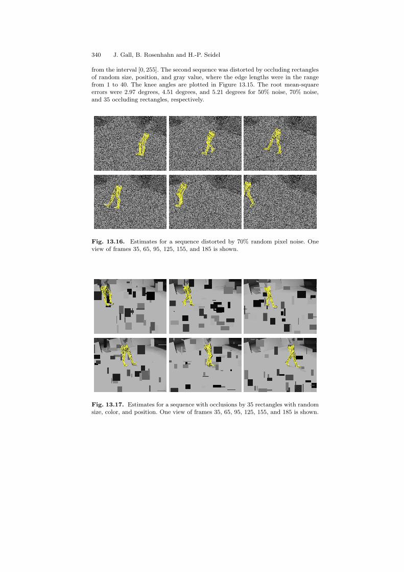
340 J. Gall, B. Rosenhahn and H.-P. Seidel
from the interval [0, 255]. The second sequence was distorted by occluding rectanglesof random size, position, and gray value, where the edge lengths were in the rangefrom 1 to 40. The knee angles are plotted in Figure 13.15. The root mean-squareerrors were 2.97 degrees, 4.51 degrees, and 5.21 degrees for 50% noise, 70% noise,and 35 occluding rectangles, respectively.
Fig. 13.16. Estimates for a sequence distorted by 70% random pixel noise. Oneview of frames 35, 65, 95, 125, 155, and 185 is shown.
Fig. 13.17. Estimates for a sequence with occlusions by 35 rectangles with randomsize, color, and position. One view of frames 35, 65, 95, 125, 155, and 185 is shown.
13 Interacting Simulated Annealing 341
13.5 Discussion
We introduced a novel approach for global optimization, termed interacting sim-ulated annealing (ISA), that converges to the global optimum. It is based on aninteracting particle system where the particles are weighted according to Boltzmann-Gibbs measures determined by an energy function and an increasing annealingscheme.The variance of the particles provides a good measure of the confidence in theestimate. If the particles are all near the global optimum, the variance is low and onlya low diffusion of the particles is required. The estimate, in contrast, is unreliable forparticles with an high variance. This knowledge is integrated via dynamic varianceschemes that focus the search on regions of interest depending on the confidence inthe current estimate. The performance and the potential of ISA was demonstratedby means of two applications.The first example showed that our approach can deal with local optima and solvesthe optimization problem well even for noisy measurements. However, we also pro-vided some limitations of the dynamic variance schemes where standard global op-timization methods might perform better. Since a comparison with other globaloptimization algorithm is out of the scope of this introduction, this will be done infuture.The application to multi-view human motion capturing, demonstrated the embed-ding of ISA into a complex system. The tracking system included silhouette ex-traction by a level-set method, a pose prediction by an auto-regression, and priorknowledge learned from training data. Providing an error analysis, we demonstratedthe accuracy and the robustness of the system in the presence of noise and occlusions.Even though we considered only a relative simple walking sequence for demonstra-tion, it already indicates the potential of ISA for human motion capturing. Indeed,a comparison with an iterative approach revealed that on the one hand global op-timization methods cannot perform better than local optimization methods whenlocal optima are not problematic as it is the case for the walking sequence, but on theother hand it also showed that the ISA can keep up with the iterative method. Weexpect therefore that the ISA performs better for faster movements, more complexmotion patterns, and human models with higher degrees of freedom. In addition,the introduced implementation of the tracking system with ISA has one essentialdrawback for the performance. While the pose estimation is performed by a globaloptimization method, the segmentation is still susceptible to local minima since theenergy function (13.29) is minimized by a local optimization approach.As part of future work, we will integrate ISA into the segmentation process to over-come the local optima problem in the whole system. Furthermore, an evaluationand a comparison with an iterative method needs to be done with sequences of dif-ferent kinds of human motions and also when the segmentation is independent ofthe pose estimation, e.g., as it is the case for background subtraction. Another im-provement might be achieved by considering correlations between the parameters ofthe particles for the dynamic variance schemes, where an optimal trade-off betweenadditional computation cost and increased accuracy needs to be found.
342 J. Gall, B. Rosenhahn and H.-P. Seidel
Acknowledgments
Our research is funded by the Max-Planck Center for Visual Computing and Com-munication. We thank Uwe Kersting for providing the walking sequence.
References
1. Ackley D. A connectionist machine for genetic hillclimbing. Kluwer, Boston,1987.
2. Back T. and Schwefel H.-P. An overview of evolutionary algorithms for param-eter optimization. Evolutionary Computation, 1:1–24, 1993.
3. Bauer H. Probability Theory. de Gruyter, Baton Rouge, 1996.4. Besl P. and McKay N. A Method for Registration of 3-D Shapes. IEEE Trans-
actions on Pattern Analysis and Machine Intelligence, 14(2):239-256, 1992.5. Brox T., Rosenhahn B., Cremers D. and Seidel H.-P.. High accuracy optical
flow serves 3-D pose tracking: exploiting contour and flow based constraints. InA.Leonardis, H.Bischof and A.Pinz, editors, European Conference on ComputerVision (ECCV), LNCS 3952, pages 98–111. Springer, 2006.
6. Brox T., Rosenhahn B., Kersting U. and Cremers D.. Nonparametric DensityEstimation for Human Pose Tracking. In Pattern Recognition (DAGM). LNCS4174, pages 546–555. Springer, 2006.
7. Bregler C., Malik J. and Pullen K. Twist Based Acquisition and Tracking ofAnimal and Human Kinematics. International Journal of Computer Vision,56:179–194, 2004.
8. Brox T., Rosenhahn B. and Weickert J. Three-dimensional shape knowledge forjoint image segmentation and pose estimation. In W.Kropatsch, R.Sablatnig,A.Hanbury, editors, Pattern Recognition (DAGM), LNCS 3663, pages 109–116.Springer, 2005.
9. Deutscher J. and Reid I. Articulated body motion capture by stochastic search.International Journal of Computer Vision, 61(2):185–205, 2005.
10. Doucet A., deFreitas N. and Gordon N., editors. Sequential Monte Carlo Meth-ods in Practice. Statistics for Engineering and Information Science. Springer,New York, 2001.
11. Gall J., Potthoff J., Schnoerr C., Rosenhahn B. and Seidel H.-P. Interactingand Annealing Particle Systems – Mathematics and Recipes. Journal of Math-ematical Imaging and Vision, 2007, To appear.
12. Gall J., Rosenhahn B. and Brox T. and Seidel H.-P. Learning for Multi-View3D Tracking in the Context of Particle Filters. In International Symposium onVisual Computing (ISVC), LNCS 4292, pages 59–69. Springer, 2006.
13. Gall J., Rosenhahn B. and Seidel H.-P. Robust Pose Estimation with 3D Tex-tured Models. In IEEE Pacific-Rim Symposium on Image and Video Technology(PSIVT), LNCS 4319, pages 84–95. Springer, 2006.
14. Geman S. and Geman D. Stochastic relaxation, Gibbs distributions and theBayesian restoration of images. IEEE Transactions on Pattern Analysis andMachine Intelligence, 6(6):721–741, 1984.
15. Gidas B. Topics in Contemporary Probability and Its Applications, Chapter 7:Metropolis-type Monte Carlo Simulation Algorithms and Simulated Annealing,pages 159–232. Probability and Stochastics Series. CRC Press, Boca Raton,1995.

13 Interacting Simulated Annealing 343
16. Goldstein H. Classical Mechanics. Addison-Wesley, Reading, MA, second edi-tion, 1980.
17. Grest D., Herzog D. and Koch R. Human Model Fitting from Monocular PostureImages. In G.Greiner, J.Hornegger, H.Niemann and M.Stamminger, editors,Vision, Modeling and Visualization. Akademische Verlagsgesellschaft Aka, 2005.
18. Kirkpatrick S., Gelatt C. Jr. and Vecchi M. Optimization by Simulated Anneal-ing. Science, 220(4598):671–680, 1983.
19. DelMoral P. Feynman-Kac Formulae. Genealogical and Interacting ParticleSystems with Applications. Probability and its Applications. Springer, NewYork, 2004.
20. Murray R.M., Li Z. and Sastry S.S. Mathematical Introduction to Robotic Ma-nipulation. CRC Press, Baton Rouge, 1994.
21. Parzen E. On estimation of a probability density function and mode. Annalsof Mathematical Statistics, 33:1065–1076, 1962.
22. Pennec X. and Ayache N. Uniform distribution, distance and expectation prob-lems for geometric features processing. Journal of Mathematical Imaging andVision, 9(1):49–67, 1998.
23. Pennec X. Computing the mean of geometric features: Application to the meanrotation. Rapport de Recherche RR–3371, INRIA, Sophia Antipolis, France,March 1998.
24. Pennec X. Intrinsic Statistics on Riemannian Manifolds: Basic Tools for Geomet-ric Measurements. Journal of Mathematical Imaging and Vision, 25(1):127–154,2006.
25. Rosenhahn B., Brox T., Cremers D. and Seidel H.-P. A Comparison ofShape Matching Methods for Contour Based Pose Estimation. In R.Reulke,U.Eckhardt, B.Flach, U.Knauer and K.Polthier, editors, 11th InternationalWorkshop on Combinatorial Image Analysis (IWCIA), LNCS 4040, pages 263–276. Springer, 2006.
26. Rosenhahn B., Brox T., Kersting U., Smith A., Gurney J. and Klette R. Asystem for marker-less human motion estimation. Kunstliche Intelligenz, 1:45–51, 2006.
27. Rosenhahn B., Brox T. and Weickert J. Three-dimensional shape knowledgefor joint image segmentation and pose tracking. In International Journal ofComputer Vision, 2006, To appear.
28. Rosenhahn B., Perwass C. and Sommer G. Pose Estimation of Free-form Con-tours. International Journal of Computer Vision, 62(3):267–289, 2005.
29. Rosenblatt F. Remarks on some nonparametric estimates of a density function.Annals of Mathematical Statistics, 27(3):832–837, 1956.
30. Szu H. and Hartley R. Fast simulated annealing. Physic Letter A, 122:157–162,1987.
31. Theobalt C., Magnor M., Schueler P. and Seidel H.-P. Combining 2D FeatureTracking and Volume Reconstruction for Online Video-Based Human MotionCapture. In 10th Pacific Conference on Computer Graphics and Applications,pages 96–103. IEEE Computer Society, 2002.
32. Tsallis C. and Stariolo D.A. Generalized simulated annealing. Physica A,233:395–406, 1996.