13 general relativity - quantum.phys.unm.edu

13

General Relativity

General relativity is built upon two of Einstein’s ideas. The first idea isthat we have no way of knowing if a particular coordinate system is correct,and so we should write our equations as tensor equations so that they are thesame in all coordinate systems. The second idea is the equivalence principleaccording to which the physics of special relativity holds inside a su�cientlysmall laboratory falling freely in an arbitrary gravitational field.

13.1 Points and their coordinates

We use coordinates to label the physical points of a spacetime and themathematical points of an abstract object. For example, we may label apoint on a sphere by its latitude and longitude with respect to a polaraxis and meridian. If we use a di↵erent axis and meridian, our coordinatesfor the point will change, but the point remains as it was. Physical andmathematical points exist independently of the coordinates we useto talk about them. When we change our system of coordinates,we change our labels for the points, but the points remain as theywere.At each point p, we can set up various coordinate systems that assign

unique coordinates xi(p) and x0i(p) to p and to points near it. For instance,polar coordinates (✓,�) are unique for all points on a sphere—except thenorth and south poles which are labeled by ✓ = 0 and ✓ = ⇡ and all0 � < 2⇡. By using a second coordinate system with ✓0 = 0 and ✓0 = ⇡on the equator in the (✓,�) system, we can assign unique coordinates to thenorth and south poles in that system. Embedding simplifies labeling. In a3-dimensional euclidian space and in the 4-dimensional Minkowski space-

13.2 Scalars 521

time in which the sphere is a surface, each point of the sphere has uniquecoordinates, (x, y, z) and (t, x, y, z).

We will use coordinate systems that represent the points of a space orspacetime uniquely and smoothly at least in local patches, so that the maps

xi = xi(p) = xi(p(x0)) = xi(x0)

x0i = x0i(p) = x0i(p(x)) = x0i(x)(13.1)

are well defined, di↵erentiable, and one to one in the patches. We’ll oftengroup the n coordinates xi together and write them collectively as x withoutsuperscripts. Since the coordinates x(p) label the point p, we sometimes willcall them “the point x.” But p and x are di↵erent. The point p is uniquewith infinitely many coordinates x, x0, x00, . . . in infinitely many coordinatesystems.We begin this chapter by noticing carefully how things change as we

change our coordinates. Our goal is to write physical theories so their equa-tions look the same in all systems of coordinates as Einstein taught us.

13.2 Scalars

A scalar is a quantity B that is the same in all coordinate systems

B0 = B. (13.2)

If it also depends upon the coordinates of the spacetime point p(x) = p(x0),then it is a scalar field, and

B0(x0) = B(x). (13.3)

Example 13.1 (Invariant squared distance) The squared distance betweenpoints separated by dxi

ds2 =3X

i=0

3X

k=0

gik(x) dxidxk (13.4)

is the same in all coordinate systems and so is a scalar. The metric gik(x)of spacetime (sections 13.13 and 13.14) compensates for the di↵erent sepa-rations dxi in di↵erent coordinate systems.In a suitably small freely falling laboratory, special relativity holds, and

so the metric gik(x) is the metric ⌘ik of special relativity (12.3), and thesquared distance between points separated by dyi in the lab’s coordinates is

522 General Relativity

ds2 =3X

i=0

3X

k=0

⌘ik dyidyk = dy · dy �

�dy0

�2. (13.5)

13.3 Contravariant vectors

By the chain rule, the change in dx0i due to changes in the unprimed coor-dinates is

dx0i =X

k

@x0i

@xkdxk. (13.6)

This transformation defines contravariant vectors: a quantity Ai is a com-ponent of a contravariant vector if it transforms like dxi

A0i =X

k

@x0i

@xkAk. (13.7)

The coordinate di↵erentials dxi form a contravariant vector. A contravariantvector Ai(x) that depends on the coordinates is a contravariant vectorfield and transforms as

A0i(x0) =X

k

@x0i

@xkAk(x). (13.8)

13.4 Covariant vectors

The chain rule for partial derivatives

@

@x0i=

X

k

@xk

@x0i@

@xk(13.9)

defines covariant vectors: a quantity Ci that transforms like a partialderivative

C 0i =

X

k

@xk

@x0iCk (13.10)

13.5 Tensors 523

is a covariant vector. A covariant vector Ci(x) that depends on the coor-dinates and transforms as

C 0i(x

0) =X

k

@xk

@x0iCk(x) (13.11)

is a covariant vector field.

Example 13.2 (Gradient of a scalar) The derivatives of a scalar fieldB0(x0) = B(x) form a covariant vector field because

@B0(x0)

@x0i=@B(x)

@x0i=

X

k

@xk

@x0i@B(x)

@xk, (13.12)

which shows that the gradient @B(x)/@xk fits the definition (13.11) of acovariant vector field.

13.5 Tensors

Tensors are structures that transform like products of vectors. A rank-zerotensor is a scalar. A rank-one tensor is a covariant or contravariant vector.Second-rank tensors are distinguished by how they transform under changesof coordinates:

covariant F 0ij =

X

k,`

@xk

@x0i@xl

@x0jFkl

contravariant M 0ij =X

k,`

@x0i

@xk@x0j

@xlMkl (13.13)

mixed N 0ij =

X

k,`

@x0i

@xk@xl

@x0jNk

l.

We can define tensors of higher rank by extending these definitions to quan-tities with more indices. The rank of a tensor also is called its order and itsdegree.

If S(x) is a scalar field, then its derivatives with respect to the coordinatesare covariant vectors (13.12) and tensors

Vi =@S

@xi, Tik =

@2S

@xi@xk, and Uik` =

@3S

@xi@xk@x`. (13.14)

The derivatives of vectors and tensors, however, are not in general tensors.An exception is the 4-curl of a covariant vector such as the Maxwell tensor


Fik = @iAk � @kAi (section 13.22). The tensorial derivatives of vectors andtensors are called covariant derivatives (sections 13.18–13.20).

Example 13.3 (Rank-2 tensors) If Ak and B` are covariant vectors, andCm and Dn are contravariant vectors, then the product Ak B` is a second-rank covariant tensor; CmDn is a second-rank contravariant tensor; andAk Cm, Ak Dn, Bk Cm, and Bk Dn are second-rank mixed tensors.

Example 13.4 (The metric tensor) The metric tensor gik(x) is a rank-2covariant tensor, so the sum

ds2 = gik(x) dxidxk (13.15)

is the same in all coordinate systems. This invariant sum has many names— invariant squared distance, interval, spacetime interval, line element —among others.

Since the transformation laws that define tensors are linear, any linearcombination (with constant coe�cients) of tensors of a given rank and kindis a tensor of that rank and kind. Thus if Fij and Gij are both second-rankcovariant tensors, so is their sum Hij = Fij +Gij .

13.6 Summation convention and contractions

An index that appears in the same monomial once as a covariant subscriptand once as a contravariant superscript, is a dummy index that is summedover

AiBi ⌘

X

i

AiBi (13.16)

usually from 0 to 3. Such a sum in which an index is repeated once covari-antly and once contravariantly is a contraction. The rank of a tensor isthe number of its uncontracted indices.Although the product Ak C` is a mixed second-rank tensor, the contrac-

tion Ak Ck is a scalar because

A0k C

0k =@x`

@x0k@x0k

@xmA`C

m =@x`

@xmA`C

m = �`mA`Cm = A`C

`. (13.17)

Similarly, the doubly contracted product F ikFik is a scalar.

13.7 Tensor equations 525

Example 13.5 (Kronecker delta) The summation convention and thechain rule imply that

@x0i

@xk@xk

@x0`=@x0i

@x0`= �i` =

⇢1 if i = `0 if i 6= `.

(13.18)

The repeated index k has disappeared in this contraction. The Kroneckerdelta �ij is a mixed second-rank tensor; it transforms as

�0i` =@x0i

@xk@xj

@x0`�kj =

@x0i

@xk@xk

@x0`=@x0i

@x0`= �i` (13.19)

and is invariant under changes of coordinates.

13.7 Tensor equations

Maxwell’s homogeneous equations (12.60) relate the derivatives of the field-strength tensor to each other as

0 = @iFjk + @kFij + @jFki. (13.20)

They are generally covariant tensor equations (sections 13.22 & 13.23).They follow from the Bianchi identity (12.88)

dF = ddA = 0. (13.21)

Maxwell’s inhomgeneous equations (12.61) relate the derivatives of the field-strength tensor to the current density ji and to the square root of the mod-ulus g of the determinant of the metric tensor gij (sections 13.13 and 13.14)

@(pg F ik)

@xk= µ0

pg ji. (13.22)

They are generally covariant tensor equations. We’ll write them as the diver-gence of a contravariant vector in section 13.31, derive them from an actionprinciple in section 13.33, and write them as invariant forms in section 14.7.Einstein’s equations (13.256) for the Ricci tensor Rik and the scalar curva-ture R in terms of the energy-momentum tensor Tik are

Rik �1

2gik R =

8⇡G

c4Tik. (13.23)

They are discussed in section 13.37.If we can write a physical law in one coordinate system as a tensor equation


Gj`(x) = 0, then in any other coordinate system the corresponding tensorequation G0ik(x0) = 0 is valid because

G0ik(x0) =@x0i

@xj@x0k

@x`Gj`(x) = 0. (13.24)

Physical laws also remain the same if expressed in terms of invariant forms.A theory written in terms of tensors or forms has equations thatare true in all coordinate systems if they are true in any coordinatesystem. Only such generally covariant theories have a chance at being rightbecause we can’t be sure that our particular coordinate system is the correctone. This is one of the key ideas of general relativity. One can make a theorythe same in all coordinate systems by applying the principle of stationaryaction (section 13.33) to an action that is invariant under all coordinatetransformations.

13.8 Inertial Frames

The other key idea of general relativity is that special relativity applies in-side a su�ciently small laboratory falling freely in an arbitrary gravitationalfield. In the inertial frame of such a falling laboratory, the physics of spe-cial relativity applies, and in particular the quadratic separation ds2 of twopoints whose coordinates are separated by dyj is the same as that measuredin any other coordinate system with distances dxi

ds2 = ⌘j` dyjdy` = ⌘j`

@yj

@xi@y`

@xkdxidxk. (13.25)

The coe�cients of dxidxk are the metric of spacetime in the other coordinatesystem

gik(x) = ⌘j`@yj(x)

@xi@y`(x)

@xk. (13.26)

This is sometimes called the principle of equivalence.

13.9 Symmetric and antisymmetric tensors

A covariant tensor is symmetric if it is independent of the order of its in-dices. That is, if Sik = Ski, then S is symmetric. Similarly a contravarianttensor Sk`m is symmetric if permutations of its indices k, `,m leave it un-changed. The metric of spacetime gik(x) = gki(x) is symmetric because itswhole role is to express infinitesimal distances as ds2 = gik(x)dxidxk whichis symmetric in i and k.

13.10 Quotient theorem 527

A covariant or contravariant tensor is antisymmetric if it changes signwhen any two of its indices are interchanged. The Maxwell field strengthFk`(x) = � F`k(x) is an antisymmetric rank-2 covariant tensor.

If T ik ✏ik = 0 where ✏12 = � ✏21 = 1 is antisymmetric, then T 12�T 21 = 0.Thus T ik ✏ik = 0 means that the tensor T ik is symmetric.

13.10 Quotient theorem

Suppose that B has unknown transformation properties, but that its prod-uct BA with all tensors A a given rank and kind is a tensor. Then B mustbe a tensor.

The simplest example is when BiAi is a scalar for all contravariant vectorsAi

B0iA

0i = BjAj . (13.27)

Then since Ai is a contravariant vector

B0iA

0i = B0i@x0i

@xjAj = BjA

j (13.28)

or✓B0

i@x0i

@xj�Bj

◆Aj = 0. (13.29)

Since this equation holds for all vectors A, we may promote it to the levelof a vector equation

B0i@x0i

@xj�Bj = 0. (13.30)

Multiplying both sides by @xj/@x0k and summing over j, we get

B0i@x0i

@xj@xj

@x0k= Bj

@xj

@x0k(13.31)

which shows that the unknown quantity Bi transforms as a covariant vector

B0k =

@xj

@x0kBj . (13.32)

The quotient rule works for tensors A and B of arbitrary rank and kind.The proof in each case is similar to the one given here.


13.11 Comma notation for derivatives

Commas are used to denote derivatives. If f(✓,�) is a function of ✓ and �,we can write its derivatives with respect to these coordinates as

f,✓ = @✓f =@f

@✓and f,� = @�f =

@f

@�. (13.33)

And we can write its double derivatives as

f,✓✓ =@2f

@✓2, f,✓� =

@2f

@✓@�, and f,�� =

@2f

@�2. (13.34)

If we use indices i, k, . . . to label the coordinates xi, xk, then we can writethe derivatives of a scalar f as

f,i = @if =@f

@xiand f,ik = @k@if =

@2f

@xk@xi(13.35)

and those of tensors T ik and Fik as

T ik,j` =

@2T ik

@xj@x`and Fik,j` =

@2Fik

@xj@x`(13.36)

and so forth.Semicolons are used to denote covariant derivatives (section 13.18).

13.12 Basis vectors and tangent vectors

A point p(x) in a spacetime with coordinates x is a scalar (13.3) because itis the same point p0(x0) = p(x0) = p(x) in all systems of coordinates x, x0,etc. Its derivatives with respect to the coordinates

@p(x)

@xi= ei(x) (13.37)

form a covariant vector ei(x)

e0i(x0) =

@p0(x0)

@x0i=@p(x)

@x0i=@xk

@x0i@p(x)

@xk=@xk

@x0iek(x) (13.38)

because p is a scalar and @i is a covariant vector. Small changes dxi in thecoordinates (in any fixed system of coordinates) lead to small changes in thepoint p(x)

dp(x) = ei(x) dxi. (13.39)

The covariant vectors ei(x) therefore form a basis (1.53) for the spacetimeat the point p(x). These basis vectors ei(x) are tangent to the curved

13.13 Metrics of Riemann Manifolds 529

spacetime at the point x and so are called tangent vectors. The manifolds,points, and vectors of this chapter are assumed to be real.

13.13 Metrics of Riemann Manifolds

A Riemann manifold of dimension d is a space that locally looks like d-dimensional euclidian space Ed and that is smooth enough for the derivatives(13.37) that define tangent vectors to exist. The surface of the Earth, forexample, looks flat at distances less than a kilometer.

Just as the surface of a sphere can be embedded in flat 3-dimensionalspace, so too every Riemann manifold can be embedded without changeof shape (isometrically) in a euclidian space En of suitably high dimen-sion (Nash, 1956). In particular, every Riemann manifold of dimension d = 3(or 4) can be isometrically embedded in a euclidian space of at most n = 14(or 19) dimensions, E14 or E19 (Gunther, 1989).

The euclidian dot products (example 1.17) of the tangent vectors (13.37)define the metric of the manifold

gik(x) = ei(x) · ek(x) =nX

↵=1

e↵i(x) e↵k(x) = ek(x) · ei(x) = gki(x) (13.40)

which is symmetric, gik(x) = gki(x). Here 1 i, k d and 1 ↵ n.The dot product of this equation is the dot product of the n-dimensionaleuclidian embedding space En.

Because the tangent vectors ei(x) are covariant vectors, the metric tensortransforms as a covariant tensor if we change coordinates from x to x0

g0ik(x0) =

@xj

@x0i@x`

@x0kgj`(x). (13.41)

The squared distance ds2 between two nearby points is the dot productof the small change dp(x) (13.39) with itself

ds2 = dp(x) · dp(x) = (ei(x) dxi) · (ek(x) dxk)

= ei(x) · ek(x) dxidxk = gik(x) dxidxk.

(13.42)

So by measuring the distances ds between nearby points, one can determinethe metric gik(x) of a Riemann space.

Example 13.6 (The sphere S2 in E3) In polar coordinates, a point p

on the 2-dimensional surface of a sphere of radius R has coordinates p =R(sin ✓ cos�, sin ✓ sin�, cos ✓) in an embedding space E3. The tangent space


E2 at p is spanned by the tangent vectors

e✓ = p,✓ =@p

@✓= R (cos ✓ cos�, cos ✓ sin�,� sin ✓)

e� = p,� =@p

@�= R (� sin ✓ sin�, sin ✓ cos�, 0).

(13.43)

The dot products of these tangent vectors are easy to compute in the em-bedding space E3. They form the metric tensor of the sphere

g =

✓g✓✓ g✓�g�✓ g��

◆=

✓e✓ · e✓ e✓ · e�e� · e✓ e� · e�

◆=

✓R2 00 R2 sin2 ✓

◆. (13.44)

Its determinant is det(gik) = R4 sin2 ✓. Since e✓ · e� = 0, the squared in-finitesimal distance (13.42) is

ds2 = e✓ · e✓ d✓2 + e� · e� d�2 = R2d✓2 +R2 sin2 ✓ d�2. (13.45)

We change coordinates from the angle ✓ to a radius r = R sin ✓/a inwhich a is a dimensionless scale factor. Then R2d✓2 = a2dr2/ cos2 ✓, andcos2 ✓ = 1� sin2 ✓ = 1� a2r2/R2 = 1� r2/L2 where L2 = (R/a)2. In thesecoordinates, the squared distance (13.45) is

ds2 =a2

1� r2/L2dr2 + a2r2 d�2 (13.46)

and the r,� metric of the sphere and its inverse are

g0 = a2✓(1� r2/L2)�1 0

0 r2

◆and g0�1 = a�2

✓1� r2/L2 0

0 r�2

◆. (13.47)

The sphere is a maximally symmetric space (section 13.26).

Example 13.7 (Graph paper) Imagine a piece of slightly crumpled graphpaper with horizontal and vertical lines. The lines give us a two-dimensionalcoordinate system (x1, x2) that labels each point p(x) on the paper. The vec-tors e1(x) = @1p(x) and e2(x) = @2p(x) define how a point moves dp(x) =ei(x) dxi when we change its coordinates by dx1 and dx2. The vectors e1(x)and e2(x) span a di↵erent tangent space at the intersection of every horizon-tal line with every vertical line. Each tangent space is like the tiny square ofthe graph paper at that intersection. We can think of the two vectors ei(x)as three-component vectors in the three-dimensional embedding space welive in. The squared distance between any two nearby points separated bydp(x) is ds2 ⌘ dp2(x) = e21(x)(dx

1)2 + 2e1(x) · e2(x) dx1dx2 + e22(x)(dx2)2

in which the inner products gij = ei(x) · ej(x) are defined by the euclidianmetric of the embedding euclidian space R3.

13.14 Metrics of Semi-Riemannian Manifolds 531

13.14 Metrics of Semi-Riemannian Manifolds

Our universe has time, and the metric ⌘ of special relativity (12.3) hasone minus sign. A semi-euclidian spacetime E(p,d�p) of dimension d is aflat spacetime with a metric that is a dot product with p minus signs andq = d � p plus signs. A semi-riemannian manifold of dimension d is aspacetime that locally looks like a semi-euclidian spacetime E(p,d�p) andthat is smooth enough for the derivatives (13.37) that define its tangentvectors to exist.

Every semi-riemannian manifold can be embedded without change ofshape (isometrically) in a semi-euclidian spacetime E(u,n�u) for su�cientlylarge u and n (Greene, 1970; Clarke, 1970). Every physically reasonable(globally hyperbolic) semi-riemannian manifold with 1 dimension of timeand 3 dimensions of space can be embedded without change of shape (iso-metrically) in a flat semi-euclidian spacetime of 1 temporal and at most 19spatial dimensions E(1,19) (Muller and Sanchez, 2011; Ake et al., 2018).The semi-euclidian dot products of the tangent vectors of an n-dimensional

semi-riemannian manifold define its metric for 0 i, k 3

gik(x) = ei(x) · ek(x) = �uX

↵=1

e↵i(x) e↵k(x) +

nX

↵=u+1

e↵i(x) e↵k(x)

= e↵i(x) e↵k(x) = e↵i(x) e↵k(x) = e↵i(x) ⇣↵� e

�k(x) = gki(x)

(13.48)

in which the metric ⇣↵� of the semi-euclidian spacetime is diagonal with

⇣↵� = ⇣↵� =

⇢�1 ↵ = � u+1 ↵ = � > u

. (13.49)

The metric (13.48) is symmetric gik(x) = gki(x).The squared distance or line element ds2 between two nearby points is

the inner product of the small change dp(x) (13.39) with itself

ds2 = dp(x) · dp(x) = e↵i(x) ⇣↵� e�k(x)dx

idxk

= ei(x) · ek(x) dxidxk = gik(x) dxidxk.

(13.50)

Thus measurements of line elements ds2 determine the metric gik(x) of thespacetime.

Some Riemann spaces have simple embeddings in semi-euclidian spaces.One example is the hyperboloid.

Example 13.8 (Hyperboloid H2) If we embed a hyperboloid H2 of radius


R in a semi-euclidian spacetime E(1,2), then a point p = (x, y, z) on the 2-dimensional surface ofH2 obeys the equation x2�R2 = y2+z2 and has polarcoordinates p = R(cosh ✓, sinh ✓ cos�, sinh ✓ sin�). The tangent vectors are

e✓ = p,✓ =@p

@✓= R (sinh ✓, cosh ✓ cos�, cosh ✓ sin�)

e� = p,� =@p

@�= R (0,� sinh ✓ sin�, sinh ✓ cos�).

(13.51)

The semi-euclidian metric of E(1,2) is ⇣ = ( � 1, 1, 1), so the inner productsare g✓,✓ = e✓ · e✓ = R2, g✓,� = e✓ · e� = 0, and g�,� = e� · e� = R2 sinh2 ✓.Thus the metric and line element of H2 are

g = R2

✓1 00 sinh2 ✓

◆and ds2 = R2 d✓2 +R2 sinh2 ✓ d�2. (13.52)

If we change coordinates from the angle ✓ to a radius r = R sinh ✓/ain which a is a dimensionless scale factor, then in terms of the parameterL2 = (R/a)2, the metric and line element (13.52) are (exercise 13.8)

g0 = a2✓(1 + r2/L2)�1 0

0 r2

◆and ds2 = a2

✓dr2

1 + r2/L2+ r2 d�2

◆.

(13.53)The hyperboloid H2 has the symmetries of the Lorentz group in one timeand two space dimensions. It is one of only three maximally symmetric(section 13.26) two-dimensional spaces. The other two are the sphere S2

(13.46) and the plane.Use of the metric (1, 1, 1) of ordinary euclidian space E3 leads to a hyper-

boloid that is not maximally symmetric (exercise 13.12).

13.15 Inverse of metric tensor

The metric g = gik is a nonsingular matrix (exercise 13.5), and so it has aninverse g�1 = gik that satisfies

g�1g = I or gik(x)gk`(x) = �i` = g0ik(x0)g0k`(x0) (13.54)

in all coordinate systems. The inverse metric gik is a rank-2 contravarianttensor (13.13) because the metric gk` is a rank-2 covariant tensor (13.41).To show this, we combine the transformation law (13.41) with the definition

13.16 Dual vectors, cotangent vectors 533

(13.54) of the inverse of the metric tensor

�i` = g0ikg0k` = g0ik@xr

@x0k@xs

@x0`grs (13.55)

and multiply both sides by

gtu@x0`

@xt@x0v

@xu. (13.56)

Use of the Kronecker-delta chain rule (13.18) now leads (exercise 13.6) to

g0iv(x0) =@x0i

@xt@x0v

@xugtu(x) (13.57)

which shows that the inverse metric gik transforms as a rank-2 contravarianttensor.

The contravariant vector Ai associated with any covariant vector Ak isdefined as Ai = gik Ak which ensures that Ai transforms contravariantly(exercise 13.7). This is called raising an index. It follows that the covari-ant vector corresponding to the contravariant vector Ai is Ak = gkiAi =gki gi`A` = �`k A` = Ak which is called lowering an index. These defini-tions apply to all tensors, so T ik` = gijgkmg`nTjmn, and so forth.

Example 13.9 (Making scalars) Fully contracted products of vectors andtensors are scalars. Two contravariant vectors Ai and Bk contracted with themetric tensor form the scalar gikAiBk = AkBk. Similarly, gikAiBk = AkBk.Derivatives of scalar fields with respect to the coordinates are covariantvectors S,i (example 13.2) and covariant tensors S,ik (section 13.5). If S isa scalar, then S,i is a covariant vector, gikS,k is a contravariant vector, andthe contraction gikS,i S,k is a scalar.

In what follows, I will often use space to mean either space or spacetime.

13.16 Dual vectors, cotangent vectors

Since the inverse metric gik is a rank-2 contravariant tensor, dual vectors

ei = gikek (13.58)

are contravariant vectors. They are orthonormal to the tangent vectors e`because

ei · e` = gikek · e` = gik gk` = �i`. (13.59)

Here the dot product is that of the embedding euclidian (13.40) or semi-euclidian (13.48) space. The dual vectors ei are called cotangent vectors


or tangent covectors. The tangent vector ek is the sum ek = gki ei because

gki ei = gki g

i` e` = �`k e` = ek. (13.60)

The definition (13.58) of the dual vectors and their orthonormality (13.59) tothe tangent vectors imply that their inner products are the matrix elementsof the inverse of the metric tensor

ei · e` = gik ek · e` = gik �`k = gi`. (13.61)

The outer product P = ekek = ekek of a tangent vector ek with itscotangent vector ek is the identity matrix of the tangent space becauseP ei = ekek · ei = ek �ki = ei and Pei = ekek · ei = ek�ik = ei

P↵� = e↵k e

k� = e↵k e�k = I↵� = �↵� . (13.62)

Details and examples are in the file tensors.pdf in Tensors and general relativityat github.com/kevinecahill.

13.17 A�ne Connection and Christo↵el Symbols

A Christo↵el symbol of the first kind �ni` is the dot product of atangent vector with the derivative of a tangent vector

�ni` = en · ei,` = e↵n ⇣↵� e�i,`. (13.63)

Since the order of derivatives of a physical point p(x) doesn’t matter, theorder of i and ` in ei,` doesn’t matter

ei,` =@2p

@xi@x`=

@2p

@x`@xi= e`,i. (13.64)

So another expression for the Christo↵el symbol is

�ni` =12

�en · ei,` + en · e`,i

�. (13.65)

We can write these dot products as

en · ei,` = gni,` � en,` · ei and en · e`,i = gn`,i � en,i · e` (13.66)

because the metric (13.48) is an inner product of tangent vectors gni = en ·ei,and gn` = en · e`. So the Christo↵el symbol is

�ni` =12

�gni,` � en,` · ei + gn`,i � en,i · e`

�. (13.67)

13.18 Covariant derivatives of contravariant vectors 535

By using again the identity (13.64) and the trick 13.66), we may write it as

�ni` =12

�gni,` + gn`,i � ei · e`,n � ei,n · e`

�

= 12

�gni,` + gn`,i � gi`,n

�.

(13.68)

Raising the index n, we get a formula for the Christo↵el symbol of thesecond kind �ki`

�ki` = gkn�ni` =12 g

kn�gni,` + gn`,i � gi`,n

�(13.69)

which is called the a�ne connection.

13.18 Covariant derivatives of contravariant vectors

The covariant derivativeD`V k of a contravariant vector V k is a derivativeof V k that transforms like a mixed rank-2 tensor. An easy way to make sucha derivative is to note that the invariant description V (x) = V i(x) ei(x) of acontravariant vector field V i(x) in terms of tangent vectors ei(x) is a scalar.Its derivative

@V

@x`=@V i

@xèi + V i @ei

@x`(13.70)

is therefore a covariant vector. And the inner product of that covariantvector V,` with a contravariant tangent vector ek is a mixed rank-2 tensorin which we recognize the a�ne connection ek · ei,` = �ki` (13.69)

D`Vk = ek · V,` = ek ·

�V i,èi + ei,`V

i�= �ki V

i,` + ek · ei,`V i

= V k,` + ek · ei,` V i = V k

,` + �ki` V

i.(13.71)

The covariant derivative itself is often written with a semicolon, thus

D`Vk = V k

;` = V k,` + ek · ei,` V i = V k

,` + �ki` V

i. (13.72)

The present notation �ki` is that of Misner, Thorne, and Wheeler (Misneret al., 1973); some other authors use �kì. But in standard formulations ofgeneral relativity �ki` = �

kì, so the di↵erence in notation doesn’t matter.

Example 13.10 (Covariant derivatives of cotangent vectors) The equation

0 = �ki,` = (ek · ei),` = ek,` · ei + ek · ei,` (13.73)


and the identity ei ei = I (13.62) imply that the covariant derivatives ofcotangent vectors vanish

D`ek = ek,` + ek · ei,` ei = ek,` � ek,` · ei ei = ek,` � ek,` = 0. (13.74)

Under general coordinate transformations, D`V k transforms as a rank-2mixed tensor

�D`V

k�0(x0) =

�V k;`�0(x0) =

@x0k

@xp@xm

@x0`V p;m(x) = x0k,px

m,`0 V

p;m(x). (13.75)

In a more explicit notation, D`V k transforms as

⇣D`V

k⌘0

=@x0k

@xp@xm

@x0`DmV p =

@x0k

@xp@xm

@x0`

✓@V p

@xm+ �pnmV n

◆

=@x0k

@xn@V n

@x0`+@x0k

@xp@xm

@x0`�pnmV n.

(13.76)

Another way to derive the form of the covariant derivative of a contravari-ant vector is as in Yang-Mills theory (Section 11.17), in which one requiresthat D0

`V0k = (D`V k)0. The condition on the connection then is that

D0`V

0k =@V 0k

@x0`+ �0km`V

0k =@

@x0`

✓@x0k

@xnV n

◆+ �0km`

@x0m

@xnV n

=@x0k

@xn@V n

@x0`+

@2x0k

@x0`@xnV n + �0km`

@x0m

@xnV n

= (D`Vk)0 =

@x0k

@xn@V n

@x0`+@x0k

@xp@xm

@x0`�pnmV n.

(13.77)

The last two lines of this equation require that

@2x0k

@x0`@xnV n + �0km`

@x0m

@xnV n =

@x0k

@xp@xm

@x0`�pnmV n (13.78)

or since V n is an arbitrary contravariant vector, that

�0km`@x0m

@xn=@x0k

@xp@xm

@x0`�pnm � @2x0k

@x0`@xn. (13.79)

Multiplying both sides by xni0 , we find that the connection �ki` must trans-form as

�0ki` =@xn

@x0i@x0k

@xp@xm

@x0`�pnm � @xn

@x0i@2x0k

@x0`@xn. (13.80)

Thus for D`V k = V k,` +�

ki` V

i to be a covariant derivative, the connection �must transform inhomogeneously, like a gauge field (11.88). Any connection

13.19 Covariant derivatives of covariant vectors 537

� that transforms this way (13.80) makes D`V k = V k,` + �

ki` V

i a covariant

derivative. The connection �ki` is not itself a tensor, but the di↵erence �0ki`��ki` between any two connections that satisfy the condition (13.80) is atensor because the inhomogeneous terms in it cancel.

The most general connection �ki` that makes D`V k = V k,` + �ki` V

i a

covariant derivative is the sum of an arbitrary rank-3 tensor T ki` and the

connection (13.69) ek · ei,`�ki` = T k

i` + ek · ei,`. (13.81)

Tangent basis vectors ei are derivatives (13.37) of the spacetime point pwith respect to the coordinates xi, and so ei,` = e`,i because partial deriva-tives commute

ei,` =@ei@x`

=@2p

@x`@xi=

@2p

@xi@x`= e`,i. (13.82)

Thus the a�ne connection (13.69) is symmetric in its lower indices

�ki` = ek · ei,` = ek · e`,i = �k`i. (13.83)

The formula (13.69) �ki` = ek · ei,` for the connection leads to a transfor-mation law

�0ki` = e0k · @e0i

@x0`=@x0k

@xp@xm

@x0`@xn

@x0i�pnm +

@x0k

@xn@2xn

@x0`@x0i

= x0k,p xm,`0 x

n,i0 �

pnm + x0k,p x

p,`0i0

(13.84)

(exercise 13.9) which is equivalent to the transformation law (13.80) (exer-cise 13.10).Since the a�ne connection �ki` is symmetric in i and `, in four-dimensional

spacetime, there are 10 �’s for each k, or 40 in all. The 10 correspond to 3rotations, 3 boosts, and 4 translations.

13.19 Covariant derivatives of covariant vectors

The derivative of the scalar V = Vk ek is the covariant vector

V,` = (Vk ek),` = Vk,` e

k + Vk ek,`. (13.85)

Its inner product with the covariant vector ei transforms as a rank-2 covari-ant tensor. Thus using again the identity (13.73), we see that the covariantderivative of a covariant vector is

D`Vi = Vi;` = ei · V,` = ei ·�Vk,` e

k + Vk ek,`�= �ki Vk,` + ei · ek,` Vk

= Vi,` � ei,` · ek Vk = Vi,` � �ki` Vk.(13.86)


D`Vi transforms as a rank-2 covariant tensor because it is the inner productof a covariant tangent vector ei with the derivative V,` of a scalar. Note that�ki` appears with a minus sign in Vi;` and a plus sign in V k

;` .

Example 13.11 (Covariant derivatives of tangent vectors) Using againthe projection matrix (13.62), we find that

Dèi = ei;` = ei,` � ei,` · ekek = ei,` � ei,` = 0 (13.87)

covariant derivatives of tangent vectors vanish.

13.20 Covariant derivatives of tensors

Tensors transform like products of vectors. So we can make the derivative ofa tensor transform covariantly by using Leibniz’s rule (5.48) to di↵erentiateproducts of vectors and by turning the derivatives of the vectors into theircovariant derivatives (13.72) and (13.86).

Example 13.12 (Covariant derivative of a rank-2 contravariant tensor)An arbitrary rank-2 contravariant tensor T ik transforms like the product oftwo contravariant vectors AiBk. So its derivative @`T ik transforms like thederivative of the product of the vectors AiBk

@`(AiBk) = (@À

i)Bk +Ai @`Bk. (13.88)

By using twice the formula (13.72) for the covariant derivative of a con-travariant vector, we can convert these two ordinary derivatives @Ài and@`Bk into tensors

D`(AiBk) = (AiBk);` = (Ai

,` + �ijÀ

j)Bk +Ai(Bk,` + �

kj`B

j)

= (AiBk),` + �ijÀ

j Bk + �kjÀiBj .

(13.89)

Thus the covariant derivative of a rank-2 contravariant tensor is

D`Tik = T ik

;` = T ik,` + �

ij` T

jk + �kj` Tij . (13.90)

It transforms as a rank-3 tensor with one covariant index.

Example 13.13 (Covariant derivative of a rank-2 mixed tensor) A rank-2 mixed tensor T i

k transforms like the product AiBk of a contravariantvector Ai and a covariant vector Bk. Its derivative @`T i

k transforms like thederivative of the product of the vectors AiBk

@`(AiBk) = (@À

i)Bk +Ai @`Bk. (13.91)

13.20 Covariant derivatives of tensors 539

We can make these derivatives transform like tensors by using the formulas(13.72) and (13.86)

D`(AiBk) = (AiBk);` = (Ai

,` + �ijÀ

j)Bk +Ai(Bk,` � �j k`Bj)

= (AiBk),` + �ijÀ

j Bk � �j kÀiBj .

(13.92)

Thus the covariant derivative of a mixed rank-2 tensor is

D` Tik= T i

k;` = T ik,` + �

ij` T

jk � �

jk` T

ij . (13.93)

It transforms as a rank-3 tensor with two covariant indices.

Example 13.14 (Covariant derivative of a rank-2 covariant tensor) Arank-2 covariant tensor Tik transforms like the product AiBk of two covari-ant vectors Ai and Bk. Its derivative @`Tik transforms like the derivative ofthe product of the vectors AiBk

@`(AiBk) = (@Ài)Bk +Ai @`Bk. (13.94)

We can make these derivatives transform like tensors by twice using theformula (13.86)

D`(AiBk) = (AiBk);` = Ai;`Bk +AiBk;`

= (Ai,` � �jiÀj)Bk +Ai(Bk,` � �j k`Bj)

= (AiBk),` � �jiÀj Bk � �j kÀiBj .

(13.95)

Thus the covariant derivative of a rank-2 covariant tensor Tik is

D` Tik = Tik;` = Tik,` � �ji` Tjk � �jk` Tij . (13.96)

It transforms as a rank-3 covariant tensor.Another way to derive the same result is to note that the scalar form of a

rank-2 covariant tensor Tik is T = ei⌦ ek Tik. So its derivative is a covariantvector

T,` = ei ⌦ ek Tik,` + ei,` ⌦ ek Tik + ei ⌦ ek,` Tik. (13.97)

Using the projector Pt = ejej (13.62), the duality ei · en = �in of tangentand cotangent vectors (13.59), and the relation ej · ek,` = � ek · ej,` = ��kj`(13.69 & 13.73), we can project this derivative onto the tangent space andfind after shu✏ing some indices

(enen ⌦ ejej)T,` = ei ⌦ ek Tik,` + en ⌦ ek (en · ei,`)Tik + ei ⌦ ej(ej · ek,`)Tik

= ei ⌦ ek Tik,` � en ⌦ ek �in` Tik � ei ⌦ ej �kj` Tik

= (ei ⌦ ek)⇣Tik,` � �ji` Tjk � �jk` Tij

⌘


which again gives us the formula (13.96).

As in these examples, covariant derivatives are derivations:

Dk(AB) = (AB);k = A;k B +AB;k = (DkA)B +ADkB. (13.98)

The rule for a general tensor is to treat every contravariant index as in(13.72) and every covariant index as in (13.86). The covariant derivative ofa mixed rank-4 tensor, for instance, is

T abxy;k = T ab

xy,k + T jbxy�

ajk + T am

xy �bmk � T ab

jy �jxk � T ab

xm�myk. (13.99)

13.21 The covariant derivative of the metric tensor vanishes

The metric tensor is the inner product (13.48) of tangent basis vectors

gik = e↵i ⇣↵� e�k (13.100)

in which ↵ and � are summed over the dimensions of the embedding space.Thus by the product rule (13.95), the covariant derivative of the metric

D` gik = gik;` = D` (e↵i ⇣↵� e

�k) = (D` e

↵i) ⇣↵� e

�k + e↵i ⇣↵� D` e

�k = 0(13.101)

vanishes because the covariant derivatives of tangent vectors vanish (13.87),D` e↵i = e↵i;` = 0 and D` e

�k = e�k;` = 0 .

13.22 Covariant curls

Because the connection �ki` is symmetric (13.83) in its lower indices, thecovariant curl of a covariant vector Vi is simply its ordinary curl

V`;i � Vi;` = V`,i � Vk �k`i � Vi,` + Vk �

ki` = V`,i � Vi,`. (13.102)

Thus the Faraday field-strength tensor Fi` = A`,i � Ai,` being the curl ofthe covariant vector field Ai is a generally covariant second-rank tensor.

13.23 Covariant derivatives and antisymmetry

The covariant derivative (13.96) Ai`;k is Ai`;k = Ai`,k�Am` �mik�Aim �m`k.If the tensor A is antisymmetric Ai` = �A`i, then by adding together thethree cyclic permutations of the indices i`k, we find that the antisymmetry

13.24 Parallel transport 541

of the tensor and the symmetry (13.83) of the a�ne connection �mik = �mki

conspire to cancel the terms with �s

Ai`;k +Aki;` +A`k;i = Ai`,k �Am` �mik �Aim �

m`k

+ Aki,` �Ami �mk` �Akm �

mi`

+ A`k,i �Amk �mì �A`m �

mki

= Ai`,k +Aki,` +A`k,i (13.103)

an identity named after Luigi Bianchi (1856–1928).The Maxwell field-strength tensor Fi` is antisymmetric by construction

(Fi` = A`,i �Ai,`), and so Maxwell’s homogeneous equations

12 ✏

ijk` Fjk,` = Fjk,` + Fk`,j + F`j,k

= Ak,j` �Aj,k` +A`,kj �Ak,`j +Aj,`k �A`,jk = 0(13.104)

are tensor equations valid in all coordinate systems.

13.24 Parallel transport

The movement of a vector along a curve on a manifold so that its lengthand direction in successive tangent spaces do not change is called paralleltransport. In parallel transport, a vector V = V k ek = Vk ek may changedV = V,` dx`, but the projection of the change P dV = eiei · dV = eiei · dVinto the tangent space must vanish, P dV = 0. In terms of its contravari-ant components V = V kek, this condition for parallel transport is just thevanishing of its covariant derivative (13.72)

0 = ei · dV = ei · V,` dx` = ei · (V kek),`dx` = ei ·

⇣V k,èk + V kek,`

⌘dx`

=⇣�ikV

k,` + ei · ek,` V k

⌘dx` =

⇣V i,` + �

ik` V

k⌘dx`.

(13.105)

In terms of its covariant components V = Vkek, the condition of paralleltransport is also the vanishing of its covariant derivative (13.86)

0 = ei · dV = ei · V,`dx` = ei · (Vkek),`dx

` = ei ·⇣Vk,è

k + Vkek,`

⌘dx`

=⇣�ki Vk,` + ei · ek,` V k

⌘dx` =

⇣Vi,` � �ki` Vk

⌘dx`.

(13.106)


If the curve is x`(u), then these conditions (13.105 & 13.106) for paralleltransport are

dV i

du= V i

,`dx`

du= � �ik` V k dx`

duand

dVi

du= Vi,`

dx`

du= �ki` Vk

dx`

du.

(13.107)

Example 13.15 (Parallel transport on a sphere) We parallel-transportthe vector v = e� = (0, 1, 0) up from the equator along the line of longitude� = 0. Along this path, the vector v = (0, 1, 0) = e� is constant, so @✓v = 0and so both e✓ ·e�,✓ = 0 and e� ·e�,✓ = 0. Thus D✓vk = vk;✓ = 0 between theequator and the north pole. As ✓ ! 0 along the meridian � = 0, the vectorv = (0, 1, 0) approaches the vector e✓ of the � = ⇡/2 meridian. We thenparallel-transport v = e✓ down from the north pole along that meridian tothe equator. Along this path, the vector v = e✓/r = (0, cos ✓,� sin ✓) obeysthe parallel-transport condition (13.106) because its ✓-derivative is

v,✓ = r�1e,✓ = (0, cos ✓,� sin ✓),✓ = � (0, sin ✓, cos ✓) = �r|�=⇡/2 .

(13.108)So v,✓ is perpendicular to the tangent vectors e✓ and e� along the curve� = ⇡/2. Thus ek · v,✓ = 0 for k = ✓ and k = � and so v;✓ = 0, alongthe meridian � = ⇡/2. When e✓ reaches the equator, it is e✓ = (0, 0,�1).Finally, we parallel-transport v along the equator back to the starting point� = 0. Along this path, the vector v = (0, 0,�1) = e✓ is constant, so v,� = 0and v;� = 0. The change from v = (0, 1, 0) to v = (0, 0,�1) is due to thecurvature of the sphere.

13.25 Curvature

To find the curvature at a point p(x0), we parallel-transport a vector Vi

along a curve x` that runs around a tiny square about the point p(x0). Wethen measure the change in the vector

�Vi =

I�ki` Vk dx

`. (13.109)

On the curve x`, we approximate the a�ne connection �ki`(x) as

�ki`(x) = �ki`(x0) + �

ki`,n(x0) (x� x0)

n (13.110)

13.25 Curvature 543

and the parallelly transported (13.107) covariant vector Vk(x) as

Vk(x) = Vk(x0) + Vk,n(x0) (x� x0)n

= Vk(x0) + �mkn(x0)Vm(x0) (x� x0)

n.(13.111)

So keeping only terms linear in (x� x0)n, we have

�Vi =

I�ki` Vk dx

` (13.112)

=h�ki`,n(x0)Vk(x0) + �

ki`(x0)�

mkn(x0)Vm(x0)

i I(x� x0)

n dx`

=h�ki`,n(x0)Vk(x0) + �

mi`(x0)�

kmn(x0)Vk(x0)

i I(x� x0)

n dx`

after interchanging the dummy indices k and m in the second term withinthe square brackets. The integral around the square is antisymmetric in nand ` and equal in absolute value to the area a2 of the tiny square

I(x� x0)

n dx` = ± a2 ✏n`. (13.113)

The overall sign depends upon whether the integral is clockwise or counter-clockwise, what n and ` are, and what we mean by positive area. The integralpicks out the part of the term between the brackets in the formula (13.112)that is antisymmetric in n and `. We choose minus signs in (13.113) so thatthe change in the vector is

�Vi = a2h�kin,` � �ki`,n + �km` �

min � �kmn �

mi`

iVk. (13.114)

The quantity between the brackets is Riemann’s curvature tensor

Rki`n = �kin,` � �ki`,n + �km` �

min � �kmn �

mi`. (13.115)

It is antisymmetric in its last two indices.

Rki`n = �Rk

in`. (13.116)

The sign convention is that of (Zee, 2013; Misner et al., 1973; Carroll,2003; Schutz, 2009; Hartle, 2003; Cheng, 2010; Padmanabhan, 2010). Wein-berg (Weinberg, 1972) uses the opposite sign. The covariant form Rijk` ofRiemann’s tensor is related to Rk

i`n by

Rijk` = ginRnjk` and Ri

jk` = ginRnjk`. (13.117)

It also is antisymmetric in its last two indices, Rijk` = �Rij`k.


The Riemann curvature tensor is the commutator of two covariant deriva-tives. To see why, we first use the formula (13.96) for the covariant derivativeDnD`Vi of the second-rank covariant tensor D`Vi

DnD`Vi = Dn

⇣Vi,` � �ki` Vk

⌘

= Vi,`n � �ki`,n Vk � �ki` Vk,n

� �jin�Vj,` � �mj`Vm

�� m`n

⇣Vi,m � �qimVq

⌘.

(13.118)

Subtracting D`DnVi, we find the commutator [Dn, D`]Vi to be the contrac-tion of the curvature tensor Rk

i`n (13.115) with the covariant vector Vk

[Dn, D`]Vi =⇣�kin,` � �ki`,n + �km` �

min � �kmn �

mi`

⌘Vk = Rk

i`n Vk.

(13.119)

Since [Dn, D`]Vi is a rank-3 covariant tensor and Vk is an arbitrary covari-ant vector, the quotient theorem (section 13.10) implies that the curvaturetensor is a rank-4 tensor with one contravariant index.If we define the matrix �` with row index k and column index i as �ki`

�` =

0

BB@

�00` �01` �02` �03`�10` �11` �12` �13`�20` �21` �22` �23`�30` �31` �32` �33`

1

CCA , (13.120)

then we may write the covariant derivatives appearing in the curvature ten-sor Rk

i`n as D` = @` + �` and Dn = @n + �n. In these terms, the curvaturetensor is the k, i matrix element of their commutator

Rki`n = [@` + �`, @n + �n]

ki = [D`, Dn]

ki . (13.121)

The curvature tensor with all lower indices has three other symmetries.In Riemann normal coordinates about any point x, the derivatives of themetric vanish at x. In these coordinates, the formulas (13.69 and 13.63) forthe �’s all vanish, and the curvature tensor Rki`n is

Rki`n = �kni,` � �k`i,n = 12

�gkn,i` � gin,k` � gk`,in + gi`,kn

�. (13.122)

In these coordinates and therefore in all coordinates, Rki`n is antisymmetricin its first two indexes and symmetric under the interchange of its first andsecond pairs of indexes

Rijk` = �Rjik` and Rijk` = Rk`ij . (13.123)

13.25 Curvature 545

Cartan’s equations of structure (13.360 & 13.362) imply (13.374) that thecurvature tensor is antisymmetric in its last three indexes

0 = Rj[ik`] =

1

3!

⇣Rj

ik` +Rjìk +Rj

kì �Rjki` �Rj

i`k �Rj`ki

⌘(13.124)

and obeys the cyclic identity

0 = Rjik` +Rj

ìk +Rjkì. (13.125)

The vanishing (13.124) of Ri[jk`] implies that the completely antisymmetricpart of the Riemann tensor also vanishes

0 = R[ijk`] =1

4!(Rijk` �Rjik` �Rikj` �Rij`k +Rjki` · · · ) . (13.126)

The Riemann tensor also satisfies a Bianchi identity

0 = Rij[k`;m]. (13.127)

These symmetries reduce 44 = 256 di↵erent functions Rijk` to 20.The Ricci tensor is the contraction

Rin = Rkikn. (13.128)

The curvature scalar is the further contraction

R = gniRin. (13.129)

Example 13.16 (Curvature of the sphere S2) While in four-dimensionalspacetime indices run from 0 to 3, on the sphere S2 (example 13.6) they arejust ✓ and �. There are only eight possible a�ne connections, and becauseof the symmetry (13.83) in their lower indices �i✓� = �i�✓, only six areindependent.In the euclidian embedding space E3, the point p on a sphere of radius

L has cartesian coordinates p = L (sin ✓ cos�, sin ✓ sin�, cos ✓), so the twotangent 3-vectors are (13.43)

e✓ = p,✓ = L (cos ✓ cos�, cos ✓ sin�, � sin ✓) = L ✓

e� = p,� = L sin ✓ (� sin�, cos�, 0) = L sin ✓ �.(13.130)

Their dot products form the metric (13.44)

g =

✓g✓✓ g✓�g�✓ g��

◆=

✓e✓ · e✓ e✓ · e�e� · e✓ e� · e�

◆=

✓L2 00 L2 sin2 ✓

◆(13.131)


which is diagonal with g✓✓ = L2 and g�� = L2 sin2 ✓. Di↵erentiating thevectors e✓ and e�, we find

e✓,✓ =� L (sin ✓ cos�, sin ✓ sin�, cos ✓) = �L r

e✓,� =L cos ✓ (� sin�, cos�, 0) = L cos ✓ �

e�,✓ =e✓,�

e�,� =� L sin ✓ (cos�, sin�, 0) .

(13.132)

The metric with upper indices gij is the inverse of the metric gij

g�1 =

✓L�2 00 L�2 sin�2 ✓

◆, (13.133)

so the dual vectors ei = gikek are

e✓ = L�1 (cos ✓ cos�, cos ✓ sin�, � sin ✓) = L�1

✓

e� =

1

L sin ✓(� sin�, cos�, 0) =

1

L sin ✓�. (13.134)

The a�ne connections are given by (13.69) as

�ijk = �ikj = ei · ej,k. (13.135)

Since both e✓ and e

� are perpendicular to r, the a�ne connections �✓✓✓and ��✓✓ both vanish. Also, e�,� is orthogonal to �, so �� = 0 as well.

Similarly, e✓,� is perpendicular to ✓, so �✓✓� = �✓�✓ also vanishes.The two nonzero a�ne connections are

��✓� = e� · e✓,� = L�1 sin�1 ✓ � · L cos ✓ � = cot ✓ (13.136)

and

�✓�� = e✓ · e�,� = � sin ✓ (cos ✓ cos�, cos ✓ sin�, � sin ✓) · (cos�, sin�, 0)

= � sin ✓ cos ✓. (13.137)

The nonzero connections are ��✓� = cot ✓ and �✓�� = � sin ✓ cos ✓. So thematrices �✓ and ��, the derivative ��,✓, and the commutator [�✓,��] are

�✓ =

✓0 00 cot ✓

◆and �� =

✓0 � sin ✓ cos ✓

cot ✓ 0

◆(13.138)

��,✓ =

✓0 sin2 ✓ � cos2 ✓

� csc2 ✓ 0

◆and [�✓,��] =

✓0 cos2 ✓

cot2 ✓ 0

◆.

Both [�✓,�✓] and [��,��] vanish. So the commutator formula (13.121) gives

13.25 Curvature 547

for Riemann’s curvature tensor

R✓✓✓✓ =[@✓ + �✓, @✓ + �✓]

✓✓ = 0

R�✓�✓ =[@� + ��, @✓ + �✓]

�✓ =

��✓,�

��✓+ [��,�✓]

�✓ = 1

R✓�✓� =[@✓ + �✓, @� + ��]

✓� = �

��✓,�

�✓�+ [�✓,��]

✓� = sin2 ✓

R�� =[@� + ��, @� + ��]

�� = 0. (13.139)

The Ricci tensor (13.128) is the contraction Rmk = Rnmnk, and so

R✓✓ = R✓✓✓✓ +R�

✓�✓ = 1

R�� = R✓�✓� +R�

�� = sin2 ✓.(13.140)

The curvature scalar (13.129) is the contraction R = gkmRmk, and so sinceg✓✓ = L�2 and g�� = L�2 sin�2 ✓, it is

R = g✓✓ R✓✓ + g��R�� = L�2 + L�2 =2

L2(13.141)

for a 2-sphere of radius L. The scalar curvature is a constant because thesphere is a maximally symmetric space (section 13.26).

Gauss invented a formula for the curvature K of a surface; for all two-dimensional surfaces, his K = R/2.

Example 13.17 (Curvature of the hyperboloid H2) The points of a hy-perboloid H2 (example 13.8) in 3-space satisfy x2 � L2 = y2 + z2 and maybe parameterized as p = L(cosh ✓, sinh ✓ cos�, sinh ✓ sin�). The coordinatebasis vectors are

e✓ = p,✓ = L(sinh ✓, cosh ✓ cos�, cosh ✓ sin�)

e� = p,� = L(0,� sinh ✓ sin�, sinh ✓ cos�).(13.142)

If the embedding metric is ⇣ = diag( � 1, 1, 1), then the squared distanceds2 between nearby points is

ds2 = e✓ · e✓ d✓2 + e� · e� d�2 = L2 d✓2 + L2 sinh2 ✓ d�2. (13.143)

The metric is

g = L2

✓1 00 sinh2 ✓

◆. (13.144)

The Mathematica scripts great.m and cylindrical hyperboloid.nb com-pute the scalar curvature as R = �2/L2. The surface is maximally symmet-ric with constant negative curvature. This chapter’s programs and scriptsare in Tensors and general relativity at github.com/kevinecahill.


Example 13.18 (Curvature of the sphere S3) The three-dimensional sphereS3 may be embedded isometrically in four-dimensional flat euclidian spaceE4 as the set of points p = (x, y, z, w) that satisfy L2 = x2 + y2 + z2 + w2.If we label its points as

p(�, ✓,�) = L(sin� sin ✓ cos�, sin� sin ✓ sin�, sin� cos ✓, cos�), (13.145)

then its coordinate basis vectors are

e� = p,� = L(cos� sin ✓ cos�, cos� sin ✓ sin�, cos� cos ✓,� sin�)

e✓ = p,✓ = L(sin� cos ✓ cos�, sin� cos ✓ sin�,� sin� sin ✓, 0)

e� = p,� = L(� sin� sin ✓ sin�, sin� sin ✓ cos�, 0, 0).

(13.146)

The inner product of E4 is the four-dimensional dot-product. The basis vec-tors are orthogonal. In terms of the radial variable r = L sin�, the squareddistance ds2 between two nearby points is

ds2 = e� · e�d�2 + e✓ · e✓d✓2 + e� · e�d�2

= L2�d�2 + sin2 � d✓2 + sin2 � sin2 ✓ d�2

�

=dr2

1� sin2 �+ r2d✓2 + r2 sin2 ✓d�2 =

dr2

1� (r/L)2+ r2d⌦2

(13.147)

where d⌦2 = d✓2 + sin2 ✓ d�2. In these coordinates, r, ✓,�, the metric is

g =

0

@1/(1� (r/L)2) 0 0

0 r2 00 0 r2 sin2 ✓

1

A . (13.148)

The Mathematica scripts great.m and sphere S3.nb compute the scalarcurvature as

R =6

L2(13.149)

which is a constant because S3 is maximally symmetric (section 13.26).If L2 = (x1)2+(x2)2+(x3)2+(x4)2 then x4dx4 = �x1dx1�x2dx2�x3dx3

and

ds2 =4X

i=1

(dxi)2 =3X

i,k=1

✓�ik +

xixk

L2 � x2

◆dxidxk (13.150)

in which x2 = (x1)2 + (x2)2 + (x3)2.

13.25 Curvature 549

Example 13.19 (Curvature of the hyperboloidH3) The hyperboloidH3 isa space of three dimensions that can be isometrically embedded in the semi-euclidian spacetime E(1,3) with a metric that is diagonal ⇣ = diag(�1, 1, 1, 1)with squared distances ds2 = dy2+dz2+dw2�dx2. The points of H3 satisfyy2 + z2 + w2 = x2 � L2. If we label them as

p(�, ✓,�) = L (cosh�, sinh� sin ✓ cos�, sinh� sin ✓ sin�, sinh� cos ✓)(13.151)

then the coordinate basis vectors or tangent vectors of H3 are

e� = p,� = L(sinh�, cosh� sin ✓ cos�, cosh� sin ✓ sin�, cosh� cos ✓)

e✓ = p,✓ = L(0, sinh� cos ✓ cos�, sinh� cos ✓ sin�,� sinh� sin ✓) (13.152)

e� = p,� = L(0,� sinh� sin ✓ sin�, sinh� sin ✓ cos�, 0).

The basis vectors are orthogonal. In terms of the radial variable r = L sinh�,the squared distance ds2 between two nearby points is

ds2 = e� · e�d�2 + e✓ · e✓d✓2 + e� · e�d�2

= L2�d�2 + sinh2 � d✓2 + sinh2 � sin2 ✓ d�2

�

=dr2

1 + sinh2 �+ r2d✓2 + r2 sin2 ✓ d�2 =

dr2

1 + (r/L)2+ r2d⌦2.

(13.153)

The Mathematica scripts great.m and hyperboloid H3.nb compute thescalar curvature of H3 as

R = � 6

L2. (13.154)

Its curvature is a constant becauseH3 is maximally symmetric (section 13.26).If L2 = (x1)2� (x2)2� (x3)2� (x4)2 then x1dx1 = x2dx2+x3dx3+x4dx4

and

ds2 =4X

i=2

(dxi)2 � (dx1)2 =4X

i,k=2

✓�ik �

xixk

L2 + x2

◆dxidxk (13.155)

in which x2 = (x2)2 + (x3)2 + (x4)2.

The hyperboloid H3 is invariant under Lorentz transformations in onetime and three space dimensions. The only maximally symmetric 3-dimensionalmanifolds are S3, H3, and euclidian space E3 whose line element is ds2 =dr2 + r2d⌦2. They are the spatial parts of Friedmann-Lemaıtre-Robinson-Walker cosmologies (section 13.44).


13.26 Maximally symmetric spaces

The spheres S2 and S3 (examples 13.6 & 13.18), the hyperboloidsH2 andH3

(examples 13.8 & 13.19), and the euclidian spaces E3 and E2 are maximallysymmetric spaces. A maximally symmetric space is a space with a maximumnumber of isometries. An isometry is a transformation x ! x0 for whichg0ik(x

0) = gik(x0) in which case the invariance g0ik(x0)dx0idx0k = gik(x)dxidxk

implies that the distances gik(x0)dx0idx0k and gik(x)dxidxk are the same.To see what this symmetry condition means, we consider the infinitesimal

transformation x0` = x` + ✏y`(x) under which to lowest order gik(x0) =gik(x)+ gik,`✏y` and dx0i = dxi+ ✏yi,jdx

j . The symmetry condition requires

gik(x)dxidxk = (gik(x) + gik,`✏y

`)(dxi + ✏yi,jdxj)(dxk + ✏yk,mdxm) (13.156)

or

0 = gik,` y` + gim ym,k + gjk y

j,i. (13.157)

The vector field yi(x) must satisfy this condition if x0i = xi + ✏yi(x) is tobe a symmetry of the metric gik(x). By using the vanishing (13.101) of thecovariant derivative of the metric tensor, we may write the condition on thesymmetry vector y`(x) as (exercise 13.11)

0 = yi;k + yk;i. (13.158)

The symmetry vector y` is a Killing vector (Wilhelm Killing, 1847–1923).We may use symmetry conditions (13.157) and (13.158) either to find thesymmetries of a space with a known metric or to find metrics with a partic-ular symmetry.

Example 13.20 (Killing vectors of the sphere S2) The first Killing vectoris (y✓1, y

�1 ) = (0, 1). Since the components of y1 are constants, the symmetry

condition (13.157) says gik,� = 0 which tells us that the metric is indepen-

dent of �. The other two Killing vectors are (y✓2, y�2 ) = (sin�, cot ✓ cos�)

and (y✓3, y�3 ) = (cos�,� cot ✓ sin�). The symmetry condition (13.157) for

i = k = ✓ and Killing vectors y2 and y3 tell us that g✓� = 0 and thatg✓✓,✓ = 0. So g✓✓ is a constant, which we set equal to unity. Finally, thesymmetry condition (13.157) for i = k = � and the Killing vectors y2 andy3 tell us that g��,✓ = 2 cot ✓g�� which we integrate to g�� = sin2 ✓. The2-dimensional space with Killing vectors y1, y2, y3 therefore has the metric(13.131) of the sphere S2.

Example 13.21 (Killing vectors of the hyperboloidH2) The metric (13.52)of the hyperboloid H2 is diagonal with g✓✓ = R2 and g�� = R2 sinh2 ✓. The

13.26 Maximally symmetric spaces 551

Killing vector (y✓1, y�1 ) = (0, 1) satisfies the symmetry condition (13.157).

Since g✓✓ is independent of ✓ and �, the ✓✓ component of (13.157) im-plies that y✓,✓ = 0. Since g�� = R2 sinh2 ✓, the �� component of (13.157)

says that y�,� = � coth ✓ y✓. The ✓� and �✓ components of (13.157) give

y✓,� = � sinh2 ✓ y�,✓. The vectors y2 = (y✓2, y�2 ) = (sin�, coth ✓ cos�) and

y3 = (y✓3, y�3 ) = (cos�, � coth ✓ sin�) satisfy both of these equations.

The Lie derivative Ly of a scalar field A is defined in terms of a vectorfield y`(x) as LyA = y`A,`. The Lie derivative Ly of a contravariant vectorF i is

LyFi = y`F i

,` � F `yi,` = y`F i;` � F `yi;` (13.159)

in which the second equality follows from y`�i`kFk = F `�i`ky

k. The Liederivative Ly of a covariant vector Vi is

LyVi = y`Vi,` + V`y`,i = y`Vi;` + V`y

`;i. (13.160)

Similarly, the Lie derivative Ly of a rank-2 covariant tensor Tik is

LyTik = y`Tik,` + T`ky`,i + Ti`y

`,k. (13.161)

We see now that the condition (13.157) that a vector field y` be a symmetryof a metric gjm is that its Lie derivative

Lygik = gik,` y` + gim ym,k + gjk y

j,i = 0 (13.162)

must vanish.A maximally symmetric space (or spacetime) in d dimensions has d trans-

lation symmetries and d(d� 1)/2 rotational symmetries which gives a totalof d(d + 1)/2 symmetries associated with d(d + 1)/2 Killing vectors. Thusfor d = 2, there is one rotation and two translations. For d = 3, there arethree rotations and three translations. For d = 4, there are six rotations andfour translations.A maximally symmetric space has a curvature tensor (13.117) that is

simply related to its metric tensor

Rijk` = c (gikgj` � gi`gjk) (13.163)

where c is a constant (Zee, 2013, IX.6). Since gkigik = gkk = d is the numberof dimensions of the space(time), the Ricci tensor (13.128) and the curvaturescalar (13.129) of a maximally symmetric space are

Rj` = gkiRijk` = c (d� 1) gj` and R = g`jRj` = c d(d� 1). (13.164)

In d dimensions, there are only three maximally symmetric spaces, the


sphere Sd, which has constant positive curvature, the hyperboloid Hd, whichhas constant negative curvature, and d-dimensional euclidean space Ed,which has curvature zero (Weinberg, 1972, ch. 13).

13.27 Principle of equivalence

Since the metric tensor gij(x) is real and symmetric, it can be diagonalized(1.379) at any point p(x) by a 4⇥ 4 orthogonal matrix O(x)

OT ki gk`O

`j =

0

BB@

e0 0 0 00 e1 0 00 0 e2 00 0 0 e3

1

CCA (13.165)

which arranges the four real eigenvalues ei of the matrix gij(x) in the ordere0 e1 e2 e3. Thus the coordinate transformation (1.381)

@xk

@x0i=

OT kip|ei|

(13.166)

takes any spacetime metric gk`(x) with one negative and three positive eigen-values into the Minkowski metric ⌘ij of flat spacetime

gk`(x)@xk

@x0i@x`

@x0j= g0ij(x

0) = ⌘ij =

0

BB@

�1 0 0 00 1 0 00 0 1 00 0 0 1

1

CCA (13.167)

at the point p(x) = p(x0).The principle of equivalence says that in these free-fall coordinates y,

the physical laws of gravity-free special relativity apply in a suitably smallregion about the point p(x) = p(y). It follows from this principle that themetric gij of spacetime accounts for all the e↵ects of gravity.In the y coordinates, the invariant squared separation dp2 is

dp2 = g0ij dyidyj = e0i(y) · e0j(y) dyidyj

= e0ai (y)⌘abe0bj (y) dy

idyj = �ai ⌘ab�bj dy

idyj

= ⌘ij dyidyj = (dy)2 � (dy0)2 = ds2.

(13.168)

If dx0 = 0, then dt0 =p�ds2/c is the proper time elapsed between events

p and p+dp. If dt0 = 0, then ds is the proper distance between the events.

13.28 Tetrads 553

The y coordinates are not unique because every Lorentz transformation(section 12.1) leaves the metric ⌘ invariant. Coordinate systems in whichgij(y) = ⌘ij are called Lorentz, inertial, or free-fall coordinate systems.The congruency transformation (1.381 & 13.165–13.167) preserves the

signs of the eigenvalues ei which make up the signature (�1, 1, 1, 1) ofthe metric tensor.

13.28 Tetrads

We defined the metric tensor as the dot product (13.40) or (13.48) of tangentvectors, gk`(x) = ek(x) ·e`(x). If instead we invert the equation (13.167) thatrelates the metric tensor to the flat metric

gk`(x) =@ya

@xk⌘ab

@yb

@x`(13.169)

then we can express the metric in terms of four 4-vectors

cak(x) =@ya

@xkas gk`(x) = cak(x) ⌘ab c

b`(x) (13.170)

in which ⌘ab is the 4 ⇥ 4 metric (13.167) of flat Minkowski space. Cartan’sfour 4-vectors cai(x) (c for Cartan) are called a moving frame, a tetrad,and a vierbein.

Example 13.22 (Tetrads of FLRW models) The metric of Friedmann,Lemaıtre, Robinson, and Walker (7.503,13.284) is diagonal with elementsgtt = �c2, grr = a2/(1�kr2/L2), g✓✓ = a2r2, and g�� = a2r2 sin2 ✓ in whicha(t) is a scale factor and L a cosmological length. It describes a cosmologyin which space is maximally symmetric (Section13.26). The tetrads

ct =

0

BB@

c000

1

CCA , cr =

0

BBB@

0ap

1�kr2/L2

00

1

CCCA, c✓ =

0

BB@

00ar0

1

CCA , c� =

0

BB@

000

ar sin ✓

1

CCA

(13.171)satisfy equations (13.169 and 13.170), but they are not unique.

Tetrads are not uniquely defined by equations (13.169 and 13.170) becauseevery (spacetime-dependent) Lorentz transformation La

c(x) ⌘ab Lbd(x) = ⌘cd


maps one set of tetrads cck(x) to another set of tetrads c0ak(x) = La

c(x) cck(x)

that represents the same metric

c0ak(x) ⌘ab c0b`(x) = La

c(x) cck(x) ⌘ab L

bd(x) c

d`(x)

= cck(x) ⌘cd cd`(x) = gk`(x).

(13.172)

Cartan’s tetrad is four 4-vectors ci that give the metric tensor as gik =ci · ck = ~ci · ~ck � c0i c

0k. The dual tetrads c i

a = gik⌘abcbk satisfy

c ia cak = gi`⌘abc

b`c

ak = gi`g`k = �ik (13.173)

Multiplying this equation from the right by c kb , we find that c i

a cakckb = c i

b

which in turn, since the tetrads c kb are linearly independent, implies that

cakckb = �ab . (13.174)

The metric gk`(x) is symmetric, gk`(x) = g`k(x), so it has 10 indepen-dent components at each spacetime point x. The four 4-vectors cak have 16components, but a Lorentz transformation L(x) has 6 components. So thetetrads have 16� 6 = 10 independent components at each spacetime point.Each tetrad cak has 4 components, a = 0, 1, 2, 3, while each tangent vector

e↵k(x) has as many components ↵ = 0, 1, 2, 3, . . . , n as there are dimensionsin the minimal semi-euclidian embedding space E1,n where n 19 (Akeet al., 2018). Another di↵erence is that the reference frame of the tetradscak(x) changes with the coordinates x, while the reference frame of thetangent vectors e↵k(x) is the embedding spacetime which remains fixed.Both represent the metric

gk`(x) =3X

a,b=0

cak(x) ⌘ab cb`(x) =

nX

↵,�=0

e↵k(x) ⇣↵� e�`(x) (13.175)

in which ⇣ is like ⌘ but with n diagonal elements that are unity.Although the 4 ⇥ 4 matrix ⌘ab occurring in these equations (13.169–

13.175) is usually taken to be the Minkowski metric of flat space (13.167),it need only be symmetric and constant as in the Newman-Penrose formal-ism (Chandrasekhar, 1998).

13.29 Scalar densities and g = | det(gik)|

Let g be the absolute value of the determinant of the metric tensor gik

g = g(x) = | det(gik(x))|. (13.176)

13.29 Scalar densities and g = | det(gik)| 555

This determinant is negative det(gik) < 0 in standard cosmologies whereg = | det(gik)| = � det(gik).Under a coordinate transformation,

pg becomes

pg0 =

pg0(y) =

q| det(g0ik(y))| =

s��det✓@xj

@yi@x`

@ykgj`(x)

◆��. (13.177)

The definition (1.213) of a determinant and the product rule (1.234) fordeterminants tell us that

pg0(y) =

s��det✓@xj

@yi

◆det

✓@x`

@yk

◆det(gj`)

�� = |J(x/y)|p

g(x) (13.178)

where J(x/y) is the jacobian (section 1.23) of the coordinate transformation

J(x/y) = det

✓@xj

@yi

◆. (13.179)

A quantity s(x) is a scalar density of weight w if it transforms as

s0(y) = [J(y/x)]ws(x). (13.180)

Thus the transformation rule (13.178) says that the determinant det(gik) isa scalar density of weight minus two

det(g0ik(y)) = = [J(x/y)]2g(x) = [J(y/x)]�2 det(gj`(x)). (13.181)

We saw in section 1.23 that under a coordinate transformation x ! y thed-dimensional element of volume in the new coordinates ddy is related tothat in the old coordinates ddx by a jacobian

ddy = J(y/x) ddx = det

✓@yi

@xj

◆ddx. (13.182)

Thus the productpg ddx changes at most by the sign of the jacobian J(y/x)

when x ! ypg0 ddy = |J(x/y)| J(y/x)

pg(x) ddx = ±

pg(x) ddx. (13.183)

The quantitypg d4x is the invariant scalar

pg |d4x| so that if L(x) is a

scalar, then the integral over spacetimeZ

L(x)pg d4x (13.184)

is invariant under general coordinate transformations. The Levi-Civita ten-sor provides a fancier definition.


13.30 Levi-Civita’s symbol and tensor

In 3 dimensions, Levi-Civita’s symbol ✏ijk ⌘ ✏ijk is totally antisymmetricwith ✏123 = 1 in all coordinate systems. In 4 space or spacetime dimensions,Levi-Civita’s symbol ✏ijk` ⌘ ✏ijk` is totally antisymmetric with ✏1234 = 1or equivalently with ✏0123 = 1 in all coordinate systems. In n dimensions,Levi-Civita’s symbol ✏i1i2...in is totally antisymmetric with ✏123...n = 1 or✏012...n�1 = 1.We can turn his symbol into a pseudotensor by multiplying it by the square

root of the absolute value of the determinant of a rank-2 covariant tensor.A natural choice is the metric tensor. In a right-handed coordinate systemin which the tangent vector e0 points (orthochronously) toward the future,the Levi-Civita tensor ⌘ijk` is the totally antisymmetric rank-4 covarianttensor

⌘ijk`(x) =p

g(x) ✏ijk` (13.185)

in which g(x) = | det gmn(x)| is (13.176) the absolute value of the deter-minant of the metric tensor gmn. In a di↵erent system of coordinates y,the Levi-Civita tensor ⌘ijk`(y) di↵ers from (13.185) by the sign s of the ja-cobian J(y/x) of any coordinate transformation to y from a right-handed,orthochronous coordinate system x

⌘ijk`(y) = s(y)pg(y) ✏ijk`. (13.186)

The transformation rule (13.178) and the definition (1.213) and product rule(1.234) of determinants show that ⌘ijk` transforms as a rank-4 covarianttensor

⌘0ijk`(y) = s(y)pg0(y) ✏ijk` = s(y) |J(x/y)|

pg(x) ✏ijk`

= J(x/y)p

g(x) ✏ijk` = det

✓@x

@x0

◆pg ✏ijk` (13.187)

=@xt

@x0i@xu

@x0j@xv

@x0k@xw

@x0`pg ✏tuvw =

@xt

@x0i@xu

@x0j@xv

@x0k@xw

@x0`⌘tuvw.

Raising the indices of ⌘ and using � as the sign of det(gik), we have

⌘ijk` = git gju gkv g`w ⌘tuvw = git gju gkv g`wpg ✏tuvw =

pg ✏ijk` det(g

mn)

=pg ✏ijk`/ det(gmn) = � ✏ijk`/

pg ⌘ � ✏ijk`/

pg. (13.188)

In terms of the Hodge star (14.151), the invariant volume element is

pg |d4x| = ⇤ 1 =

1

4!⌘ijk` dx

i ^ dxj ^ dxk ^ dx`. (13.189)

13.31 Divergence of a contravariant vector 557

13.31 Divergence of a contravariant vector

The contracted covariant derivative of a contravariant vector is a scalarknown as the divergence,

r · V = V i;i = V i

,i + V k �iki. (13.190)

Because gik = gki, in the sum over i of the connection (13.69)

�iki =12g

i`�gi`,k + g`k,i � gki,`

�(13.191)

the last two terms cancel because they di↵er only by the interchange of thedummy indices i and `

gi`g`k,i = gìgik,` = gi`gki,`. (13.192)

So the contracted connection collapses to

�iki =12g

i`gi`,k. (13.193)

There is a nice formula for this last expression. To derive it, let g ⌘ gi` bethe 4⇥4 matrix whose elements are those of the covariant metric tensor gi`.Its determinant, like that of any matrix, is the cofactor sum (1.222) alongany row or column, that is, over ` for fixed i or over i for fixed `

det(g) =X

i or `

gi`Ci` (13.194)

in which the cofactor Ci` is (�1)i+` times the determinant of the reducedmatrix consisting of the matrix g with row i and column ` omitted. Thusthe partial derivative of det g with respect to the i`th element gi` is

@ det(g)

@gi`= Ci` (13.195)

in which we allow gi` and gì to be independent variables for the purposesof this di↵erentiation. The inverse gi` of the metric tensor g, like the inverse(1.224) of any matrix, is the transpose of the cofactor matrix divided by itsdeterminant det(g)

gi` =Cì

det(g)=

1

det(g)

@ det(g)

@gì. (13.196)


Using this formula and the chain rule, we may write the derivative of thedeterminant det(g) as

det(g),k =@ det(g)

@gi`gi`,k = det(g) g`i gi`,k (13.197)

and so since gi` = g`i, the contracted connection (13.193) is

�iki =12g

i`gi`,k =det(g),k2 det(g)

=| det(g)|,k2| det(g)| =

g,k2g

=(pg),kpg

(13.198)

in which g⌘��det(g)

�� is the absolute value of the determinant of the metrictensor.Thus from (13.190 & 13.198), we arrive at our formula for the covariant

divergence of a contravariant vector:

r · V = V i;i = V i

,i + �ikiV

k = V k,k +

(pg),kpg

V k =(pg V k),kp

g. (13.199)

Example 13.23 (Maxwell’s inhomogeneous equations) An important ap-plication of this divergence formula (13.199) is the generally covariant form(14.157) of Maxwell’s inhomogeneous equations

1pg

⇣pgF k`

⌘

,`= µ0j

k. (13.200)

Example 13.24 (Energy-momentum tensor) Another application is to thedivergence of the symmetric energy-momentum tensor T ij = T ji

T ij;i = T ij

,i + �iki Tkj + �jmi T

im

=(pgT kj)kp

g+ �jmi T

im.(13.201)

13.32 Covariant laplacian

In flat 3-space, we write the laplacian as r ·r = r2 or as 4. In euclidiancoordinates, both mean @2x + @2y + @2z . In flat minkowski space, one oftenturns the triangle into a square and writes the 4-laplacian as 2 = 4� @20 .The gradient f,k of a scalar field f is a covariant vector, and f ,i = gikf,k

is its contravariant form. The invariant laplacian 2f of a scalar field f

13.33 Stationary action and geodesic equation 559

is the covariant divergence f,i;i . We may use our formula (13.199) for the

divergence of a contravariant vector to write it in these equivalent ways

2f = f,i;i = (gikf,k);i =

(pg f ,i),ipg

=(pg gikf,k),ip

g. (13.202)

13.33 Stationary action and geodesic equation

The invariant proper time for a particle to move along a path xi(t)

T =

Z ⌧2

⌧1

d⌧ =1

c

Z ⇣� gi`dx

idx`⌘ 1

2=

1

c

Z ✓� gi`

dxi

d⌧

dx`

d⌧

◆ 12

d⌧ (13.203)

is extremal and stationary on free-fall paths called geodesics. The actionT is invariant under reparametrization ⌧ ! �(⌧) since

Z ✓� gi`

dxi

d�

dx`

d�

◆ 12

d� =

Z ✓� gi`

dxi

d⌧

d⌧

d�

dx`

d⌧

d⌧

d�

◆ 12 d�

d⌧d⌧

=

Z ✓� gi`

dxi

d⌧

dx`

d⌧

◆ 12

d⌧.

(13.204)

We can identify a geodesic by computing the variation �d⌧

c�d⌧ = �p�gi`dxidx` =

��(gi`)dxidx` � 2gi`dxi�dx`

2p�gi`dxidx`

(13.205)

= �gi`,k2c

�xkuiu`d⌧ � gi`cui�dx` = �

gi`,k2c

�xkuiu`d⌧ � gi`cuid�x`

in which u` = dx`/d⌧ is the 4-velocity (12.31). The path is extremal if

0 = c�T = c

Z ⌧2

⌧1

�d⌧ = � 1

c

Z ⌧2

⌧1

✓12gi`,k�x

kuiu` + gi`uid�x

`

d⌧

◆d⌧ (13.206)

which we integrate by parts keeping in mind that �x`(⌧2) = �x`(⌧1) = 0

0 = �Z ⌧2

⌧1

✓12gi`,k�x

kuiu` � d(gi`ui)

d⌧�x`

◆d⌧

= �Z ⌧2

⌧1

✓12gi`,k�x

kuiu` � gi`,kuiuk�x` � gi`

dui

d⌧�x`

◆d⌧. (13.207)

Now interchanging the dummy indices ` and k on the second and third


terms, we have

0 = �Z ⌧2

⌧1

✓12gi`,ku

iu` � gik,ùiu` � gik

dui

d⌧

◆�xkd⌧ (13.208)

or since �xk is arbitrary

0 = 12gi`,ku


dui

d⌧. (13.209)

If we multiply this equation of motion by grk and note that gik,ùiu` =g`k,iuiu`, then we find

0 =dur

d⌧+ 1

2grk

�gik,` + g`k,i � gi`,k

�uiu`. (13.210)

So using the symmetry gi` = gì and the formula (13.69) for �ri`, we get

0 =dur

d⌧+ �ri` u

iu` or 0 =d2xr

d⌧2+ �ri`

dxi

d⌧

dx`

d⌧(13.211)

which is the geodesic equation. In empty space, particles fall along geodesicsindependently of their masses. Equation (13.209) also is useful in theform

d

d⌧

�gki u

i�=

1

2gi`,k u

i u`. (13.212)

Example 13.25 (A flat expanding universe) In a spatially flat expandinguniverse (Sections 7.46 and 13.44), ds2 = �c2dt2 + a2(dr2 + r2d⌦2). So thegeodesic equation (13.212) for a particle moving in the radial j = r directionis

d

d⌧(grru

r) =d

d⌧

�a2ur

�= 2a

da

d⌧ur + a2

dur

d⌧= 0. (13.213)

Integrating dur/ur = �2da/a, we get ur = ur0/a2. The physical velocity is

vr = a dr/dt, and �ds2 = c2d⌧2 = (c2 � v2)dt2, so d⌧ =p1� v2/c2 dt. So

in a flat expanding universe the momentum falls o↵ as 1/a

p =mvp

1� v2/c2=

map1� v2/c2

dr

dt= ma

dr

d⌧= maur =

mur0a

=p0a

(13.214)in which p0 = mur0 is the momentum when a = a0 = 1.

One can also get the geodesic equations (13.211 and 13.212) from thesimpler action principle

0 = �

Z ⌧2

⌧1

gi`(x)ui u` d⌧ = �

Z ⌧2

⌧1

gi`(x)dxi

d⌧

dx`

d⌧d⌧. (13.215)

13.33 Stationary action and geodesic equation 561

Using primes to denote di↵erentiation with respect to ⌧ , we find

0 =

Z ⌧2

⌧1

hgi`,k �x

k (xi)0 (x`)0 + gi` (�xi)0(x`)0 + gi` (x

i)0(�x`)0id⌧

=

Z ⌧2

⌧1

hgi`,k (x

i)0 (x`)0 � (gk` (x`)0)0 � (gik (x

i)0)0i�xk d⌧

(13.216)

which implies that

0 =�gi`,k � gk`,i � gik,`

�(x`)0(xi)0 � 2g`k (x

`)00 (13.217)

or

0 = (xr)00 + 12 g

rk�gk`,i + gik,` � gi`,k

�(x`)0(xi)0

0 =d2xr

d⌧2+ �ri`

dxi

d⌧

dx`

d⌧.

(13.218)

The right-hand side of the geodesic equation (13.211) is a contravariantvector because (Weinberg, 1972) under general coordinate transformations,the inhomogeneous terms arising from (xr)00 cancel those from �ri`(x

i)0(x`)0.The action for a particle of mass m and charge q in a gravitational field

�ri` and an electromagnetic field Ai is

S = �mc

Z ⇣� gi`dx

idx`⌘ 1

2+

q

c

Z ⌧2

⌧1

Ai(x) dxi (13.219)

in which the interaction qRAidxi is invariant under general coordinate trans-

formations. By (12.74 & 13.208), the first-order change in S is

�S = m

Z ⌧2

⌧1

12gi`,ku


dui

d⌧+

q

mc

�Ai,k �Ak,i

�ui��xkd⌧

(13.220)and so by combining the Lorentz force law (12.75) and the geodesic equation(13.211) and by writing F ri(xi)0 as F r

i (xi)0, we have

0 =d2xr

d⌧2+ �ri`

dxi

d⌧

dx`

d⌧� q

mF r

idxi

d⌧(13.221)

as the equation of motion of a particle of mass m and charge q. It is strikinghow nearly perfect the electromagnetism of Faraday and Maxwell is.

The action of the electromagnetic field interacting with an electric currentjk in a gravitational field is

S =

Z h�1

4 Fk` Fk` + µ0Ak j

kip

g d4x (13.222)


in whichpg d4x is the invariant volume element. After an integration by

parts, the first-order change in the action is

�S =

Z � @

@x`

⇣F k`pg

⌘+ µ0 j

k pg

��Ak d

4x, (13.223)

and so the inhomogeneous Maxwell equations in a gravitational field are

@

@x`

⇣pg F k`

⌘= µ0

pg jk. (13.224)

The action of a scalar field � of mass m in a gravitational field is

S =1

2

Z ⇣� �,i g

ik�,k �m2�2⌘p

g d4x. (13.225)

After an integration by parts, the first-order change in the action is

�S =

Z��

⇣pg gik�,k

⌘

,i�m2pg �

�d4x (13.226)

which yields the equation of motion⇣p

g gik�,k⌘

,i�m2pg � = 0. (13.227)

In a flat universe expanding with scale factor a(t) (13.284 with k = 0) andHubble rate H = a/a, this equation of motion is

�+ 3H�� a�2r2�+m2� = 0. (13.228)

The action of the gravitational field itself is a spacetime integral of theRiemann scalar (13.129) divided by Newton’s constant

S =c3

16⇡G

ZRpg d4x. (13.229)

Its variation leads to Einstein’s equations (section 13.37).

13.34 Equivalence principle and geodesic equation

The principle of equivalence (section 13.27) says that in any gravitationalfield, one may choose free-fall coordinates in which all physical laws takethe same form as in special relativity without acceleration or gravitation—atleast over a suitably small volume of spacetime. Within this volume and inthese coordinates, things behave as they would at rest deep in empty spacefar from any matter or energy. The volume must be small enough so that

13.34 Equivalence principle and geodesic equation 563

the gravitational field is constant throughout it. Such free-fall coordinatesystems are called local Lorentz frames and local inertial frames.

Example 13.26 (Elevators) When a modern elevator starts going downfrom a high floor, it accelerates downward at something less than the lo-cal acceleration of gravity. One feels less pressure on one’s feet; one feelslighter. After accelerating downward for a few seconds, the elevator assumesa constant downward speed, and then one feels the normal pressure of one’sweight on one’s feet. The elevator seems to be slowing down for a stop, butactually it has just stopped accelerating downward.

What if the cable snapped, and a frightened passenger dropped his laptop?He could catch it very easily as it would not seem to fall because the elevator,the passenger, and the laptop would all fall at the same rate. The physicsin the falling elevator would be the same as if the elevator were at rest inempty space far from any gravitational field. The laptop’s clock would tickas fast as it would at rest in the absence of gravity, but to an observer onthe ground it would appear slower.

What if a passenger held an electric charge? Observers in the falling el-evator would see a static electric field around the charge, but observers onthe ground would see radiation from the accelerating charge.

Example 13.27 (Proper time) An interval d⌧ of proper time in a giveninertial frame (where special relativity applies) is the time measured by aclock at rest dy = 0 in that frame so that � (dy0)2 = �c2d⌧2 = ds2. Inany other coordinates xi the invariant ds2 is ds2 = gik(x) dxidxk, so in thosecoordinates the proper time interval is

d⌧ =1

c

q�gik(x) dxidxk. (13.230)

Example 13.28 (Clock hypothesis) The apparent lifetime of an unstableparticle is independent of the acceleration of the particle even when theparticle is subjected to centripetal accelerations of 1019 m/s2(Bailey et al.,1977) and to longitudinal accelerations of 1016m/s2(Roos et al., 1980).

The transformation from arbitrary coordinates xk to free-fall coordinatesyi changes the metric gj` to the diagonal metric ⌘ik of flat spacetime ⌘ =diag(�1, 1, 1, 1), which has two indices and is not a Levi-Civita tensor. Al-gebraically, this transformation is a congruence (1.383)

⌘ik =@xj

@yigj`

@x`

@yk. (13.231)


The geodesic equation (13.211) follows from the principle of equiva-lence (Weinberg, 1972; Hobson et al., 2006). Suppose a particle is movingunder the influence of gravitation alone. Then one may choose free-fall co-ordinates y(x) so that the particle obeys the force-free equation of motion

d2yi

d⌧2= 0 (13.232)

with d⌧ the proper time d⌧2 = �⌘ik dyidyk. The chain rule applied to yi(x)in (13.232) gives

0 =d

d⌧

✓@yi

@xkdxk

d⌧

◆

=@yi

@xkd2xk

d⌧2+

@2yi

@xk@x`dxk

d⌧

dx`

d⌧. (13.233)

We multiply by @xm/@yi and use the identity

@xm

@yi@yi

@xk= �mk (13.234)

to write the equation of motion (13.232) in the x-coordinates

d2xm

d⌧2+ �mk`

dxk

d⌧

dx`

d⌧= 0. (13.235)

This is the geodesic equation (13.211) in which the a�ne connection is

�mk` =@xm

@yi@2yi

@xk@x`. (13.236)

13.35 Weak static gravitational fields

Newton’s equations describe slow motion in a weak static gravitational field.Because the motion is slow, we neglect ui compared to u0 and simplify thegeodesic equation (13.211) to

0 =dur

d⌧+ �r00 (u

0)2. (13.237)

Because the gravitational field is static, we neglect the time derivatives gk0,0and g0k,0 in the connection formula (13.69) and find for �r00

�r00 =12 g

rk�g0k,0 + g0k,0 � g00,k

�= �1

2 grk g00,k (13.238)

13.36 Gravitational time dilation 565

with �000 = 0. Because the field is weak, the metric can di↵er from ⌘ij byonly a tiny tensor gij = ⌘ij + hij so that to first order in |hij | ⌧ 1 wehave �r00 = �1

2 h00,r for r = 1, 2, 3. With these simplifications, the geodesicequation (13.211) reduces to

d2xr

d⌧2= 1

2 (u0)2 h00,r or

d2xr

d⌧2=

1

2

✓dx0

d⌧

◆2

h00,r. (13.239)

So for slow motion, the ordinary acceleration is described by Newton’s law

d2x

dt2=

c2

2rh00. (13.240)

If � is his potential, then for slow motion in weak static fields

g00 = �1 + h00 = �1� 2�/c2 and so h00 = � 2�/c2. (13.241)

Thus, if the particle is at a distance r from a mass M, then � = � GM/rand h00 = �2�/c2 = 2GM/rc2 and so

d2x

dt2= �r� = r GM

r= �GM

r

r3. (13.242)

How weak are the static gravitational fields we know about? The dimen-sionless ratio �/c2 is 10�39 on the surface of a proton, 10�9 on the Earth,10�6 on the surface of the sun, and 10�4 on the surface of a white dwarf.

13.36 Gravitational time dilation

Our formula (13.230) for an interval d⌧ of proper time (example 13.27) is

d⌧ =1

c

p�gik dxidxk. (13.243)

So the proper time of a clock at rest in the weak, static gravitational field(13.237–13.242) is

d⌧ =p�g00 dt =

p1 + 2�/c2 dt. (13.244)

So the ratio of the proper-time intervals measured by clocks in the Earth’sgravitational field �(r) = �GM/r at r + h and at r is

d⌧(r + h)

d⌧(r)=

p1 + 2�(r + h)/c2p1 + 2�(r)/c2

⇡ 1 +gh

c2(13.245)

in which g = GM/r2 = 9.807 m s�2. The lower clock is slower.


Example 13.29 (Pound and Rebka) Pound and Rebka in 1960 used theMossbauer e↵ect to measure the blue shift of light falling down a 22.6 mshaft. They found �⌫/⌫ = gh/c2 = 2.46 ⇥ 10�15. (Robert Pound 1919–2010, Glen Rebka 1931–2015) media.physics.harvard.edu/video/?id=

LOEB_POUND_092591.flv

Example 13.30 (Redshift of the sun) A photon emitted with frequency ⌫0at a distance r from a mass M would be observed at spatial infinity to havefrequency ⌫ = ⌫0

p�g00 = ⌫0

p1� 2MG/c2r for a redshift of �⌫ = ⌫0 � ⌫.

Since the Sun’s dimensionless potential ��/c2 is �MG/c2r = �2.12⇥ 10�6

at its surface, sunlight is shifted to the red by 2 parts per million.

13.37 Einstein’s equations

If we make an action that is a scalar, invariant under general coordinatetransformations, and then apply to it the principle of stationary action, wewill get tensor field equations that are invariant under general coordinatetransformations. If the metric of spacetime is among the fields of the action,then the resulting theory will be a possible theory of gravity. If we make theaction as simple as possible, it will be Einstein’s theory.To make the action of the gravitational field, we need a scalar. Apart from

the scalarpg d4x =

pg c dt d3x, where g = | det(gik)|, the simplest scalar

we can form from the metric tensor and its first and second derivatives isthe scalar curvature R which gives us the Einstein-Hilbert action

SEH =c3

16⇡G

ZRpg d4x =

c3

16⇡G

Zgik Rik

pg d4x (13.246)

in which G = 6.7087⇥ 10�39 ~c (GeV/c2)�2 = 6.6743⇥ 10�11m3 kg�1 s�2 isNewton’s constant.If �gik(x) is a tiny local change in the inverse metric, then the rule

� detA = detATr(A�1�A) (1.237), valid for any nonsingular, nondefectivematrix A, together with the identity 0 = �(gikgk`) = �gik gk` + gik �gk` andthe notation g for the metric tensor gj` considered as a matrix imply that

�pg =

det g

2gpg� det g =

(det g)2gik �gik2g

pg

= � 1

2

pg gik �g

ik. (13.247)

13.37 Einstein’s equations 567

So the first-order change in the action density is

�⇣gik Rik

pg⌘= Rik

pg �gik + gik Rik �

pg + gik

pg �Rik

=

✓Rik �

1

2Rgik

◆pg �gik + gik

pg �Rik.

(13.248)

The product gik�Rik is a scalar, so we can evaluate it in any coordinatesystem. In a local inertial frame, where �abc = 0 and gde is constant, thisinvariant variation of the Ricci tensor (13.128) is

gik�Rik = gik ��nin,k � �nik,n

�= gik (@k ��

nin � @n ��

nik)

= gik @k ��nin � gin @k ��

kin = @k

⇣gik ��nin � gin ��kin

⌘.

(13.249)

The transformation law (13.84) for the a�ne connection shows that thevariations ��nin and ��kin are tensors although the connections themselvesaren’t. Thus, we can evaluate this invariant variation of the Ricci tensorin any coordinate system by replacing the derivatives with covariant onesgetting

gik�Rik =⇣gik ��nin � gin ��kin

⌘

;k(13.250)

which we recognize as the covariant divergence (13.199) of a contravariantvector. The last term in the first-order change (13.248) in the action densityis therefore a surface term whose variation vanishes for tiny local changes�gik of the metric

pg gik�Rik =

hpg⇣gik ��nin � gin ��kin

⌘i

,k. (13.251)

Hence the variation of SEH is simply

�SEH =c3

16⇡G

Z ✓Rik �

1

2gikR

◆pg �gik d4x. (13.252)

The principle of least action �SEH = 0 now gives us Einstein’s equationsfor empty space:

Rik �1

2gik R = 0. (13.253)

The tensor Gik = Rik � 12gik R is Einstein’s tensor.

Taking the trace of Einstein’s equations (13.253), we find that the scalarcurvature R and the Ricci tensor Rik are zero in empty space:

R = 0 and Rik = 0. (13.254)


The energy-momentum tensor Tik is the source of the gravitationalfield. It is defined so that the change in the action of the matter fields dueto a tiny local change �gik(x) in the metric is

�Sm = � 1

2c

ZTik

pg �gik d4x =

1

2c

ZT ik pg �gik d

4x (13.255)

in which the identity �gik = � gijg`k�gj` explains the sign change. Now theprinciple of least action �S = �SEH + �Sm = 0 yields Einstein’s equationsin the presence of matter and energy

Gik ⌘ Rik �1

2gik R =

8⇡G

c4Tik (13.256)

in which Gik is the Einstein tensor. Taking the trace of both sides, we get

R = � 8⇡G

c4T and Rik =

8⇡G

c4

✓Tik �

T

2gik

◆. (13.257)

13.38 Energy-momentum tensor

The action Sm of the matter fields �i is a scalar that is invariant undergeneral coordinate transformations. In particular, a tiny local general coor-dinate transformation x0a = xa + ✏a(x) leaves Sm invariant

0 = �Sm =

Z�⇣L(�i(x))

pg(x)

⌘d4x. (13.258)

The vanishing change �Sm = �Sm� + �Smg has a part �Sm� due to thechanges in the fields ��i(x) and a part �Smg due to the change in the metric�gik. The principle of stationary action tells us that the change �Sm� iszero as long as the fields obey the classical equations of motion. Combiningthe result �Sm� = 0 with the definition (13.255) of the energy-momentumtensor, we find

0 = �Sm = �Sm� + �Smg = �Smg =1

2c

ZT ik pg �gik d

4x. (13.259)

13.39 Perfect fluids 569

Since xa = x0a � ✏a(x), the transformation law for rank-2 covariant tensors(13.41) gives us

�gik = g0ik(x)� gik(x) = g0ik(x0)� gik(x)� (g0ik(x

0)� g0ik(x))

= (�ai � ✏a,i)(�bk � ✏b,k)gab � gik � ✏cgik,c

= � gib ✏b,k � gak ✏

a,i � ✏c gik,c

= � gib(gbc ✏c),k � gak(g

ac ✏c),i � ✏c gik,c

= � ✏i,k � ✏k,i � ✏c gib gbc,k � ✏c gak g

ac,i � ✏c gik,c.

(13.260)

Now using the identity @i(gik gk`) = 0, the definition (13.86) of the covariantderivative of a covariant vector, and the formula (13.69) for the connectionin terms of the metric, we find to lowest order in the change ✏a(x) in xa thatthe change in the metric is

�gik = � ✏i,k � ✏k,i + ✏c gbc gib,k + ✏c g

ac gak,i � ✏c gik,c

= � ✏i,k � ✏k,i + ✏c gac�gia,k + gak,i � gik,a

�

= � ✏i,k � ✏k,i + ✏c �cik + ✏c �

cki = � ✏i;k � ✏k;i.

(13.261)

Combining this result (13.261) with the vanishing (13.259) of the change�Smg, we have

0 =

ZT ik pg (✏i;k + ✏k;i) d

4x. (13.262)

Since the energy-momentum tensor is symmetric, we may combine the twoterms, integrate by parts, divide by

pg, and so find that the covariant di-

vergence of the energy-momentum tensor is zero

0 = T ik;k = T ik

,k + �kak Tia + �iak T

ak =1pg(pgT ik),k + �

iak T

ak (13.263)

when the fields obey their equations of motion. In flat space, this equationsays that the energy and momentum of the matter fields are conserved,0 = T ik

,k . The analog of T ab for the gravitational field is not a tensor; it’s

a pseudotensor tab (Dirac, 1975). The divergence of (T ab + tab)pg vanishes

because the action does not depend upon an external spacetime point. Butthe spatial integrals for the energy and momentum of the gravitational fieldmay lie at infinity or diverge.

13.39 Perfect fluids

In many cosmological models, the energy-momentum tensor is assumed tobe that of a perfect fluid, which is isotropic in its rest frame, does not


conduct heat, and has zero viscosity. The energy-momentum tensor Tij

of a perfect fluid moving with 4-velocity ui (12.31) is

Tij = p gij + (p

c2+ ⇢)ui uj (13.264)

in which p and ⇢ are the pressure and mass density of the fluid in its restframe and gij is the spacetime metric. Einstein’s equations (13.256) thenare

Rik �1

2gik R =

8⇡G

c4Tik =

8⇡G

c4

hp gij + (

p

c2+ ⇢)ui uj

i. (13.265)

An important special case is the energy-momentum tensor due to a nonzerovalue of the energy density of the vacuum. In this case p = �c2⇢ and theenergy-momentum tensor is

Tij = p gij = �c2⇢ gij (13.266)

in which c2⇢ is the value of the energy density of the ground state of thetheory. This energy density c2⇢ is a plausible candidate for the dark-energydensity. It is equivalent to a cosmological constant ⇤ = 8⇡G⇢.

On small scales, such as that of our solar system, one may neglect mat-ter and dark energy. So in empty space and on small scales, the energy-momentum tensor vanishes Tij = 0 along with its trace and the scalar cur-vature T = 0 = R, and Einstein’s equations (13.257) are

Rij = 0. (13.267)

13.40 Gravitational waves

The nonlinear properties of Einstein’s equations (13.256– 13.257) are im-portant on large scales of distance (sections 13.44 & 13.44) and near greatmasses (sections 13.41 & 13.42). But throughout most of the mature uni-verse, it is helpful to linearize them by writing the metric as the metric ⌘ikof empty, flat spacetime (12.3) plus a tiny deviation hik

gik = ⌘ik + hik. (13.268)

To first order in hik, the a�ne connection (13.69) is

�ki` =12 g

kj�gji,` + gj`,i � gi`,j

�= 1

2 ⌘kj�hji,` + hj`,i � hi`,j

�(13.269)

13.41 Schwarzschild and Eddington Metrics 571

and the Ricci tensor (13.128) is the contraction

Ri` = Rkik` = [@k + �k, @` + �`]

ki = �

k`i,k � �kki,`. (13.270)

Since �ki` = �k`i and hik = hki, the linearized Ricci tensor is

Ri` =12 ⌘

kj�hji,` + hj`,i � hi`,j

�,k �

12 ⌘

kj�hji,k + hjk,i � hik,j

�,`

= 12

⇣hk`,ik + h

,kik,` � h

,ki`,k � hkk,i`

⌘. (13.271)

We can simplify Einstein’s equations (13.257) in empty space Ri` = 0 byusing coordinates in which hik obeys (exercise 13.19) de Donder’s harmonicgauge condition hik,i = 1

2(⌘j`hj`),k ⌘ 1

2h,k. In this gauge, the linearizedEinstein equations in empty space are

Ri` = � 12 h

,ki`,k = 0 or

�c2r2 � @20

�hi` = 0. (13.272)

In 2015, the LIGO collaboration detected the merger of two black holesof 29 and 36 solar masses which liberated 3M�c2 of energy. They have setan upper limit of c2mg < 2 ⇥ 10�25 eV on the mass of the graviton, havedetected 10 black-hole mergers, and are expected to detect a new mergerevery week in late 2019.

13.41 Schwarzschild and Eddington Metrics

In 1916, Schwarzschild solved Einstein’s field equations (13.267) in emptyspace Rij = 0 outside a static, spherically symmetric mass M . He found

ds2 = �✓1� 2GM

c2r

◆c2dt2 +

✓1� 2GM

c2r

◆�1

dr2 + r2 d⌦2, (13.273)

in which d⌦2 = d✓2 + sin2 ✓ d�2. The Mathematica scripts great.m andSchwarzschild.nb show that the Schwarzschild metric obeys Einstein’s equa-tions (13.253) for empty space Rik = 0 and R = 0.Eddington set r = [1+GM/(2c2r0)]2r0 and got for the metric outside the

Schwarzschild radius rS = 2GM/c2

ds2 = ��1� GM

2c2r0

�2�1 + GMe

2c2r0

�2 c2dt2 +

✓1 +

GM

2c2r0

◆4

(dr02 + r02d⌦2) (13.274)

in which r0 =px2 + y2 + z2 and dr02+r02d⌦2 = dx2+dy2+dz2 (Eddington,

1924). His metric is isotropic with the speed of light the same in all directions.


The proper time d⌧ measured by a clock at rest at r in Schwarzschild’scoordinates

d⌧ =

r1� 2GM

c2rdt (13.275)

is less than that d⌧ = dt measured by a clock at rest far from the mass M .At the Schwarzschild radius r = rS = 2GM/c2 the clock stops; light emittedby an atom at rS is red-shifted to zero frequency as it gets far from the blackhole. (Karl Schwarzschild 1873–1916, Arthur Eddington 1882–1944)

13.42 Black holes

Suppose an uncharged, static, spherically symmetric star of mass M has col-lapsed to within a sphere of radius less than rS = 2GM/c2 in Schwarzschild’scoordinates. Then outside the star, the metrics (13.273 and 13.274) apply,and light emitted by the star is red-shifted to zero frequency far from thestar. The star is a black hole. If the radius of the Sun, 6.957⇥ 105 km, wereless than its Schwarzschild radius of 2.95 km, the Sun would be a black hole.Black holes are not black. They often are surrounded by bright hot accre-

tion disks, and Stephen Hawking showed (Hawking, 1975) that the intensegravitational field of a black hole of mass M radiates at a temperature thatis inversely proportional to the mass of the star

T =~ c3

8⇡ kB GM(13.276)

in which kB = 8.617⇥10�5 eV K�1 is Boltzmann’s constant, and ~ = 1.055⇥10�34 J s.In a region of empty space where the pressure p and the chemical poten-

tials µj vanish, the change (7.115) in the internal energy U = c2M of a blackhole of mass M is dU = c2dM = TdS where S is its entropy. So the changedS in the entropy of a black hole of mass M and temperature T (13.276) is

dS =c2

TdM =

8⇡kBGMdM

~c . (13.277)

Integrating, we get a formula for the entropy of a black hole in terms ofits mass and also in terms of the areas of its Schwarzschild AS = 4⇡r2

Sand

Eddington AE = 4⇡r2Ehorizons (Bekenstein, 1973)

S =4⇡kBGM2

~c =c3kB

4~G AS =4c3kB

~G AE. (13.278)

The entropy of a black hole of 60 solar masses is about 4⇥ 1057.

13.43 Rotating black holes 573

A black hole radiates energy according to the Stefan-Boltzmann law (5.111)

c2dM

dt= �AT 4 = �4⇡r2

ST 4 =

~ c615360⇡G2M2

. (13.279)

Integrating, we see that a black hole is entirely converted into radiation aftera time

t =5120⇡G2

~ c4 M3 (13.280)

proportional to the cube of its mass M . (Stephen Hawking 1942–2018)

13.43 Rotating black holes

A half-century after Einstein invented general relativity, Roy Kerr found themetric for a mass M rotating with angular momentum J = cMa. Two yearslater, Newman and others generalized the Kerr metric to one of charge q. InBoyer-Lindquist coordinates, its line element is

ds2 = � �

⇢2�c dt� a sin2 ✓d�

�2

+sin2 ✓

⇢2�(r2 + a2)d�� a c dt

�2+⇢2

�dr2 + ⇢2d✓2

= �✓1� 2GMr/c2 �Q2

⇢2

◆c2dt2 � 2a sin2 ✓ (2GMr/c2 �Q2)

⇢2c dt d�

+(r2 + a2)2 � a2� sin2 ✓

⇢2sin2 ✓ d�2 +

⇢2

�dr2 + ⇢2d✓2 (13.281)

in which ⇢2 = r2 + a2 cos2 ✓ and � = r2 � 2GMr/c2 + a2 +Q2. Here Q2 =Gq2/(4⇡✏0c4) and q is the charge in Coulombs. The Mathematica scriptKerr black hole.nb shows that the Kerr-Newman metric for the unchargedcase, q = 0, has Rik = 0 and R = 0, and so is a solution of Einstein’sequations in empty space (13.257) with zero scalar curvature.A rotating mass drags nearby masses along with it. The daily rotation

of the Earth drags satellites to the East by tens of meters per year. Theframe dragging of extremal black holes can approach the speed of light.(Roy Kerr 1934–, Ezra Newman 1929–2021)


13.44 Friedmann-Lemaıtre-Robinson-Walker Cosmologies

Einstein’s equations (13.257) are second-order, nonlinear partial di↵erentialequations for 10 unknown functions gik(x) in terms of the energy-momentumtensor Tik(x) throughout the universe, which of course we don’t know. Theproblem is not quite hopeless, however. The ability to choose arbitrary co-ordinates, the appeal to symmetry, and the choice of a reasonable form forTik all help.Astrophysical observations tell us that the universe extends at least 46

billion light years in all directions; that it is flat or very nearly flat; andthat the cosmic microwave background (CMB) radiation is isotropic to onepart in 105 apart from a Doppler shift due the motion of the Sun at 370km/s towards the constellation Leo. These microwave photons have beenmoving freely since the universe became cool enough for hydrogen atoms tobe stable. Observations of clusters of galaxies reveal an expanding universethat is homogeneous on suitably large scales of distance. Thus as far as weknow, the universe is homogeneous and isotropic in space, but not intime.There are only three maximally symmetric 3-dimensional spaces: eu-

clidian space E3, the sphere S3 (example 13.18), and the hyperboloid H3

(example 13.19). Their line elements may be written in terms of a distanceL as

ds2 =dr2

1� k r2/L2+ r2d⌦2 or ds2 =

✓�ik +

k xixk

L2 � k x2

◆dxidxk (13.282)

in which k = 1 for the sphere, k = 0 for euclidian space, k = � 1 forthe hyperboloid, and i and k are summed from 1 to 3. The Friedmann-Lemaıtre-Robinson-Walker (FLRW) cosmologies add to these spatiallysymmetric line elements a dimensionless scale factor a(t) that describesthe expansion (or contraction) of space

ds2 = � c2dt2 + a2(t)

✓dr2

1� k r2/L2+ r2 d✓2 + r2 sin2 ✓ d�2

◆. (13.283)

The FLRW metric is

gik(t, r, ✓,�) =

0

BB@

� c2 0 0 00 a2/(1� k r2/L2) 0 00 0 a2 r2 00 0 0 a2 r2 sin2 ✓

1

CCA . (13.284)

The constant k determines whether the spatial universe is open k = � 1,flat k = 0, or closed k = 1. The coordinates x0, x1, x2, x3 ⌘ t, r, ✓,� are

13.44 Friedmann-Lemaıtre-Robinson-Walker Cosmologies 575

comoving in that a detector at rest at r, ✓,� records the CMB as isotropicwith no Doppler shift. If k = 0 or L = 1, we may use ordinary rectangularcomoving coordinates x = (x, y, z) with ds2 = �c2dt2 + a2dx · dx.The metric (13.284) is diagonal; its inverse gij also is diagonal

gik =

0

BB@

� c�2 0 0 00 (1� k r2/L2)/a2 0 00 0 (a r)�2 00 0 0 (a r sin ✓)�2

1

CCA . (13.285)

One may compute the a�ne connection (13.69) from the metric and itsinverse as �ki` = 1

2gkj(gji,` + gj`,i � g`i,j). It usually is easier, however,

to use the action principle (13.20) to derive the geodesic equation directlyand then to read its expressions for the �ijk’s. So we require that 0 =

�R�gik(xi)0(xk)0 d⌧ in which a prime means derivative with respect to ⌧ .

That is, we require that

0 = �

Z ✓�c2t02 +

a2 r02

1� kr2/L2+ a2 r2 ✓02 + a2 r2 sin2 ✓ �02

◆d⌧ (13.286)

to first order in arbitrary tiny variations �t(⌧), �r(⌧), �✓(⌧), and ��(⌧).

Example 13.31 (Variation of t(⌧)) After an integration by parts, thevanishing of the variation (13.286) when only t(⌧) is varied gives us

0 =

Z 2c2t00 + 2aa

✓r02

1� kr2/L2+ r2 ✓02 + r2 sin2 ✓ �02

◆��t d⌧. (13.287)

Setting the term within the square brackets equal to zero and using thegeodesic equation (13.20), we get

0 = t00+aa

c2

✓r02

1� kr2/L2+ r2 ✓02 + r2 sin2 ✓ �02

◆= t00+�ti`x

0ix0` (13.288)

which tells us that the nonzero �tjk’s are

�trr =aa

c2(1� kr2/L2), �t✓✓ =

aa r2

c2, and �t�� =

aa r2 sin2 ✓

c2.

(13.289)

By varying r(⌧) we get (with more e↵ort)

0 = r00 +rr02k/L2

(1� kr2/L2)+ 2

a t0r0

a� r (1� kr2

L2)(✓02 + sin2 ✓ �02). (13.290)


So we find that �rtr = a/a,

�rrr =kr

L2 � kr2, �r✓✓ = � r+

kr3

L2, and �r�� = sin2 ✓ �r✓✓. (13.291)

Varying ✓(⌧) gives

0 = ✓00 + 2a

at0✓0 +

2

r✓0r0 � sin ✓ cos ✓�02 and

�✓t✓ =a

a, �✓r✓ =

1

r, and �✓�� = � sin ✓ cos ✓.

(13.292)

Finally, varying �(⌧) gives

0 = �00 + 2a

at0�0 + 2

r0�0

r+ 2 cot ✓ ✓0�0 and

��t� =a

a, ��r� =

1

r, and ��✓� = cot ✓.

(13.293)

Other �’s are either zero or related by the symmetry �ki` = �k`i.

Our formulas for the Ricci (13.128) and curvature (13.121) tensors give

R00 = Rk0k0 = [Dk, D0]

k0 = [@k + �k, @0 + �0]

k0. (13.294)

Because [D0, D0] = 0, we need only compute [D1, D0]10, [D2, D0]20, and[D3, D0]30. Using the formulas (13.289–13.293) for the �’s and keeping inmind (13.120) that the element of row r and column c of the `th gammamatrix is �r`c, we find

[D1, D0]10 = �

100,1 � �110,0 + �11j�

j00 � �

10j�

j10 = � (a/a),0 � (a/a)2

[D2, D0]20 = �

200,2 � �220,0 + �22j�

j00 � �

20j�

j20 = � (a/a),0 � (a/a)2

[D3, D0]30 = �

300,3 � �330,0 + �33j�

j00 � �

30j�

j30 = � (a/a),0 � (a/a)2

Rtt = R00 = [Dk, D0]k0 = � 3(a/a),0 � 3(a/a)2 = � 3a/a. (13.295)

Thus for Rrr = R11 = Rk1k1 = [Dk, D1]k1 = [@k + �k, @1 + �1]k1, we get

Rrr = [Dk, D1]k1 =

aa+ 2a2 + 2kc2/L2

c2(1� kr2/L2)(13.296)

(exercise 13.25), and for R22 = R✓✓ and R33 = R�� we find

R✓✓ = [(aa+ 2a2 + 2kc2/L2)r2]/c2 and R�� = sin2 ✓R✓✓ (13.297)

13.45 Friedmann Equations 577

(exercises 13.26 & 13.27). And so the scalar curvature R = gabRba is

R = gabRba = � R00

c2+

(1� kr2/L2)R11

a2+

R22

a2r2+

R33

a2r2 sin2 ✓

= 6aa+ a2 + kc2/L2

c2a2. (13.298)

It is, of course, quicker to use the Mathematica script FLRW.nb. (AlexanderFriedmann, 1888–1925; Georges Lemaıtre, 1894–1966; Howard Robinson,1903–1961; Arthur Walker, 1909–2001)

13.45 Friedmann Equations

The energy-momentum tensor (13.264) of a perfect fluid moving at 4-velocityui is Tik = pgik + (p/c2 + ⇢)uiuk where p and ⇢ are the pressure and massdensity of the fluid in its rest frame. In the comoving coordinates xi =(t, r, ✓,�) of the FLRW metric (13.284), the 4-velocity ui = dxi/d⌧ (12.31)is ui = (1, 0, 0, 0), and the energy-momentum tensor (13.264) is

Tij =

0

BB@

�c2⇢ g00 0 0 00 p g11 0 00 0 p g22 00 0 0 p g33

1

CCA . (13.299)

Its trace is

T = gij Tij = �c2⇢+ 3p. (13.300)

Thus using our formulas (13.284) for g00 = � c2, (13.295) for R00 = �3a/a,(13.299) for Tij , and (13.300) for T , we can write the 00 Einstein equation(13.257) as the second-order equation

a

a= �4⇡G

3

✓⇢+

3p

c2

◆(13.301)

which is nonlinear because ⇢ and p depend upon a. The sum c2⇢ + 3p de-termines the acceleration a of the scale factor a(t); when it is negative, itaccelerates the expansion. If we combine Einstein’s formula for the scalarcurvature R = �8⇡GT/c4 (13.257) with the FLRW formulas for R (13.298)and for the trace T (13.300) of the energy-momentum tensor, we get

a

a+

✓a

a

◆2

+c2k

L2a2=

4⇡G

3

✓⇢� 3p

c2

◆. (13.302)

Using the 00-equation (13.301) to eliminate the second derivative a, we find


✓a

a

◆2

=8⇡G

3⇢ � c2k

L2a2(13.303)

which is a first-order nonlinear equation. It and the second-order equation(13.301) are known as the Friedmann equations.The left-hand side of the first-order Friedmann equation (13.303) is the

square of the Hubble rate

H =a

a(13.304)

which is an inverse time or a frequency. Its present value H0 is the Hubbleconstant.In terms of H, the first-order Friedmann equation (13.303) is

H2 =8⇡G

3⇢� c2k

L2a2. (13.305)

A spatially flat universe has k = 0; so the mass density ⇢ of a spatially flatFLRW universe is always equal to critical mass density

⇢ = ⇢c ⌘3H2

8⇡G. (13.306)

In terms of these densities and their ratio ⌦ = ⇢/⇢c, the Friedmann equation(13.305) says that

c2k

L2H2a2=

⇢

⇢c� 1 = ⌦� 1 (13.307)

and thus that closed (k > 0) universes have ⌦ > 1, flat (k = 0) universeshave ⌦ = 1, and open (k < 0) universes have ⌦ < 1.

13.46 Density and pressure

For i = 0, the vanishing of the covariant divergence of the energy-momentumtensor (13.263) is

0 = T 0a;a = @aT

0a + �acaT0c + �0caT

ca. (13.308)

For a perfect fluid of 4-velocity ua, the energy-momentum tensor (13.299)is T ik = (⇢ + p/c2)uiuk + pgik in which ⇢ and p are the mass density andpressure of the fluid in its rest frame. The comoving frame of the Friedmann-Lemaıtre-Robinson-Walker metric (13.284) is the rest frame of the fluid. Inthese coordinates, the 4-velocity ua is (1, 0, 0, 0), and the energy-momentum

13.46 Density and pressure 579

tensor is diagonal with T 00 = ⇢ and T jj = pgjj for j = 1, 2, 3. Our connectionformulas (13.289) tell us that �000 = 0, that �0jj = agjj/(c2a), and that

�j0j = 3a/a. Thus the conservation law (13.308) becomes for spatial j

0 = @0T00 + �j0jT

00 + �0jjTjj

= ⇢+ 3a

a⇢+

3X

j=1

a gjjc2a

p gjj = ⇢+ 3a

a

⇣⇢+

p

c2

⌘ (13.309)

a result that also follows from Friedmann’s equations (exercise 13.32). Thuswe may write the conservation of energy as

⇢ = � 3a

a(⇢+

p

c2) () d⇢

da= �3

a

⇣⇢+

p

c2

⌘. (13.310)

The mass density ⇢ is composed of fractions ⇢i each contributing its ownpartial pressure pi according to its own equation of state

pi = c2wi⇢i (13.311)

in which wi is a constant. The rate of change (13.311) of the mass density⇢i is then

d⇢ida

= � 3

a(1 + wi) ⇢i. (13.312)

In terms of the present density ⇢i0 and scale factor a0, the solution is

⇢i = ⇢i0⇣a0a

⌘3(1+wi). (13.313)

There are three important kinds of density. The mass density ⇢⇤ of dark-energy is assumed to be like a cosmological constant ⇤ or like the energydensity of the vacuum, so it is independent of the scale factor a and hasw⇤ = �1.

A universe composed only of dust or non-relativistic collisionlessmatter has no pressure. Thus p = w⇢ = 0 with ⇢ 6= 0, and so w = 0.So the matter density falls inversely with the volume

⇢m = ⇢m0

⇣a0a

⌘3. (13.314)

The density of radiation ⇢r has wr = 1/3 because wavelengths scale withthe scale factor, and so there’s an extra factor of a

⇢r = ⇢r0⇣a0a

⌘4. (13.315)


The total density ⇢ varies with a as

⇢ = ⇢⇤ + ⇢m0

⇣a0a

⌘3+ ⇢r0

⇣a0a

⌘4. (13.316)

This mass density ⇢, the Friedmann equations (13.301 & 13.303), and thephysics of the standard model have caused our universe to evolve as inFig. 13.1 over the past 14 billion years.

13.47 How the scale factor evolves with time

History of the universe

Figure 13.1 NASA/WMAP Science Team’s timeline of the known universe.

The first-order Friedmann equation (13.303) expresses the square of theinstantaneous Hubble rate H = a/a in terms of the density ⇢ and the scalefactor a(t)

H2 =

✓a

a

◆2

=8⇡G

3⇢� c2k

L2a2(13.317)

in which k = ±1 or 0. The critical density ⇢c = 3H2/(8⇡G) (13.306) is theone that satisfies this equation for a flat (k = 0) universe. Its present value is⇢c0 = 3H2

0/(8⇡G) = 8.599 ⇥ 10�27 kg m�3. Dividing Friedmann’s equation

13.47 How the scale factor evolves with time 581

by the square of the present Hubble rate H20 , we get

H2

H20

=1

H20

✓a

a

◆2

=1

H20

✓8⇡G

3⇢� c2k

a2L2

◆=

⇢

⇢0c� c2k

a2H20L

2(13.318)

in which ⇢ is the total density (13.316)

H2

H20

=⇢⇤⇢c0

+⇢m⇢c0

+⇢r⇢c0

� c2k

a2H20L

2

=⇢⇤⇢c0

+⇢m0

⇢c0

a30a3

+⇢r0⇢c0

a40a4

� c2k

a20H20L

2

a20a2

.

(13.319)

The Planck collaboration use a model in which the energy density ofthe universe is due to radiation, matter, and a cosmological constant ⇤.Only about 18.79% of the matter in their model is composed of baryons,⌦b = 0.05845±0.0003. Most of the matter is transparent and is called darkmatter. They assume the dark matter is composed of particles that havemasses in excess of a keV so that they are heavy enough to have been nonrela-tivistic or “cold” when the universe was about a year old (Peebles, 1982). Theenergy density of the cosmological constant ⇤ is known as dark energy. ThePlanck collaboration use this ⇤-cold-dark-matter (⇤CDM) model and theirCMB data to estimate the Hubble constant as H0 = 67.66 km/(sMpc) =2.1927⇥ 10�18 s�1 and the density ratios ⌦⇤ = ⇢⇤/⇢c0, ⌦m = ⇢m0/⇢c0, and⌦k ⌘ �c2k/(a0H0L)2 as listed in the table (13.1) (Aghanim et al., 2018).The Riess group use the Gaia observatory to calibrate Cepheid stars andtype Ia supernovas as standard candles for measuring distances to remotegalaxies. The distances and redshifts of these galaxies give the Hubble con-stant as H0 = 73.48 ± 1.66 (Riess et al., 2018). As this book goes to press,the 9% discrepancy between the Planck and Riess H0’s is unexplained.

Table 13.1 Cosmological parameters of the Planck collaboration

H0 (km/(s Mpc) ⌦⇤ ⌦m ⌦k

67.66± 0.42 0.6889± 0.0056 0.3111± 0.0056 0.0007± 0.0037

To estimate the ratio ⌦r = ⇢r0/⇢c0 of densities, one may use the presenttemperature T0 = 2.7255 ± 0.0006 K (Fixsen, 2009) of the CMB radiationand the formula (5.110) for the mass density of photons

⇢� =8⇡5 (kBT0)

4

15h3c5= 4.6451⇥ 10�31 kg m�3. (13.320)

Adding in three kinds of neutrinos and antineutrinos, which decoupled before


the positrons annihilated with electrons and so are at the lower temperatureT0⌫ = (4/11)1/3 T0, we get for the present density of massless and nearlymassless particles (Weinberg, 2010, section 2.1)

⇢r0 =

"1 + 3

✓7

8

◆✓4

11

◆4/3#⇢� = 7.8099⇥ 10�31 kg m�3. (13.321)

The fraction ⌦r of the present critical mass density that is due to radiationis then

⌦r =⇢r0⇢c0

= 9.0824⇥ 10�5. (13.322)

In terms of ⌦r and of the ⌦’s in the table (13.1), the formula (13.319) forH2/H2

0 is

H2

H20

= ⌦⇤ + ⌦ka20a2

+ ⌦ma30a3

+ ⌦ra40a4

. (13.323)

Since H = a/a, one has dt = da/(aH) = H�10 (da/a)(H0/H), and so with

x = a/a0, the time interval dt is

dt =1

H0

dx

x

1p⌦⇤ + ⌦k x�2 + ⌦m x�3 + ⌦r x�4

. (13.324)

Integrating and setting the origin of time t(0) = 0 and the scale factor atthe present time equal to unity a0 = 1, we find that the time t(a) that a(t)took to grow from 0 to a(t) is

t(a) =1

H0

Z a

0

dxp⌦⇤ x2 + ⌦k + ⌦m x�1 + ⌦r x�2

. (13.325)

This integral gives the age of the universe as t(1) = 13.789 Gyr; the Planck-collaboration value is 13.787±0.020 Gyr (Aghanim et al., 2018). Figure 13.2plots the scale factor a(t) and the redshift z(t) = 1/a � 1 as functions ofthe time t (13.325) for the first 14 billion years after the time t = 0 ofinfinite redshift. A photon emitted with wavelength � at time t(a) now haswavelength �0 = �/a(t). The change in its wavelength is �� = � z(t) =� (1/a� 1) = �0 � �.

13.48 The first hundred thousand years

Figure 13.3 plots the scale factor a(t) as given by the integral (13.325) andthe densities of radiation ⇢r(t) and matter ⇢m(t) for the first 100,000 yearsafter the time of infinite redshift. Because wavelengths grow with the scalefactor, the radiation density (13.315) is proportional to the inverse fourth

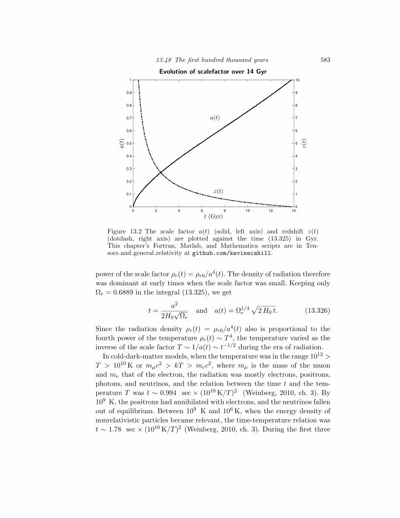
13.48 The first hundred thousand years 583

Evolution of scalefactor over 14 Gyr

0 2 4 6 8 10 12 14

0

0.1

0.2

0.3

0.4

0.5

0.6

0.7

0.8

0.9

1

0

1

2

3

4

5

6

7

8

9

10

Figure 13.2 The scale factor a(t) (solid, left axis) and redshift z(t)(dotdash, right axis) are plotted against the time (13.325) in Gyr.This chapter’s Fortran, Matlab, and Mathematica scripts are in Ten-sors and general relativity at github.com/kevinecahill.

power of the scale factor ⇢r(t) = ⇢r0/a4(t). The density of radiation thereforewas dominant at early times when the scale factor was small. Keeping only⌦r = 0.6889 in the integral (13.325), we get

t =a2

2H0p⌦r

and a(t) = ⌦1/4r

p2H0 t. (13.326)

Since the radiation density ⇢r(t) = ⇢r0/a4(t) also is proportional to thefourth power of the temperature ⇢r(t) ⇠ T 4, the temperature varied as theinverse of the scale factor T ⇠ 1/a(t) ⇠ t�1/2 during the era of radiation.

In cold-dark-matter models, when the temperature was in the range 1012 >T > 1010K or mµc2 > kT > mec2, where mµ is the mass of the muonand me that of the electron, the radiation was mostly electrons, positrons,photons, and neutrinos, and the relation between the time t and the tem-perature T was t ⇠ 0.994 sec ⇥ (1010K/T )2 (Weinberg, 2010, ch. 3). By109 K, the positrons had annihilated with electrons, and the neutrinos fallenout of equilibrium. Between 109 K and 106K, when the energy density ofnonrelativistic particles became relevant, the time-temperature relation wast ⇠ 1.78 sec ⇥ (1010K/T )2 (Weinberg, 2010, ch. 3). During the first three


Evolution of scalefactor and densities over first 100 kyr

0 10 20 30 40 50 60 70 80 90 100

0

0.5

1

1.5

2

2.5

3

3.5

4

4.510

-4

0

0.5

1

1.5

2

2.5

3

3.5

4

4.5

510

-16

Figure 13.3 The Planck-collaboration scale factor a (solid), radiation den-sity ⇢r (dotdash), and matter density ⇢m (dashed) are plotted as functionsof the time (13.325) in kyr. The era of radiation ends at t = 50, 506 yearswhen the two densities are equal to 1.0751⇥10�16 kg/m3, a = 2.919⇥10�4,and z = 3425.

minutes (Weinberg, 1988) of the era of radiation, quarks and gluons formedhadrons, which decayed into protons and neutrons. As the neutrons decayed(⌧ = 877.7 s), they and the protons formed the light elements—principallyhydrogen, deuterium, and helium in a process called big-bang nucleosyn-thesis.The density of nonrelativistic matter (13.314) falls as the third power

of the scale factor ⇢m(t) = ⇢m0/a3(t). The more rapidly falling density ofradiation ⇢r(t) crosses it 50,506 years after the Big Bang as indicated bythe vertical line in the figure (13.3). This time t = 50, 506 yr and redshiftz = 3425 mark the end of the era of radiation.

13.49 The next ten billion years

The era of matter began about 50,506 years after the time of infiniteredshift when the matter density ⇢m first exceeded the radiation density ⇢r.Some 330,000 years later at t ⇠ 380, 000 yr, the universe had cooled to aboutT = 3000 K or kT = 0.26 eV—a temperature at which less than 1% of the

13.50 Era of dark energy 585

hydrogen was ionized. At this redshift of z = 1090, the plasma of ions andelectrons became a transparent gas of neutral hydrogen and helium withtrace amounts of deuterium, helium-3, and lithium-7. The photons emittedor scattered at that time as 0.26 eV or 3000 K photons have redshifteddown to become the 2.7255 K photons of the cosmic microwave background(CMB) radiation. This time of last scattering and first transparency is calleddecoupling.During 330,000 of the 380,000 years between the time of infinite redshift

and the time of first transparency, the dominant energy density was that ofmatter. During those 330,000 years, photons strongly scattered o↵ electronswhich interacted strongly with nuclei. The photons, electrons, and baryonsformed a dense interacting plasma in which disturbances propagated at whatis called the speed of sound, nearly vs ⇡ c/

p3. If we approximate time

periods t� tm during the era of matter by keeping only ⌦m in the integral(13.325), then we get

t� tm =2 a3/2

3H0p⌦m

and a(t) =

✓3H0

p⌦m (t� tm)

2

◆2/3

+ a(tm).

(13.327)in which t is a time well inside the era of matter and tm ⇠ 50,000 years.

Between 10 and 17 million years after the Big Bang, the temperature ofthe known universe fell from 373 to 273 K. If by then the supernovas ofvery early, very heavy stars had produced carbon, nitrogen, and oxygen,biochemistry may have started during this period of 7 million years. Starsdid form at least as early as 180 million years after the Big Bang (Bowmanet al., 2018).

The era of matter lasted until the energy density of matter ⇢m(t), fallingas ⇢m(t) = ⇢m0/a3(t), had dropped to the energy density of dark energy⇢⇤ = 5.9238 ⇥ 10�27kg/m3. This happened at t = 10.228 Gyr as indicatedby the first vertical line in the figure (13.4).

13.50 Era of dark energy

The era of dark energy began when the energy density of matter ⇢m droppedbelow the energy density of empty space ⇢⇤ = 5.9238 ⇥ 10�27 kg/m3. Thishappened 3.6 billion years ago at a redshift of z = 0.3034. The decelerationof the expansion of the universe became acceleration much earlier. The ac-celeration a is given by Friedmann’s second-order equation (13.301) and maybe written in terms of the pressures of dark energy p⇤ = �c2⇢⇤, radiation


Evolution of scalefactor and densities over 50 Gyr

0 5 10 15 20 25 30 35 40 45 50

0

1

2

3

4

5

6

7

8

9

0

0.1

0.2

0.3

0.4

0.5

0.6

0.7

0.8

0.9

110

-26

Figure 13.4 The scale factor a (solid), the vacuum density ⇢⇤ (dotdash),and the matter density ⇢m (dashed) are plotted as functions of the time(13.325) in Gyr. The era of matter ends at t = 10.228 Gyr (first vertical line)when the two densities are equal to 5.9238⇥ 10�27kg m�3 and a = 0.7672.The present time t0 is 13.787 Gyr (second vertical line) at which a(t) = 1.

pr = c2⇢r/3, and matter pm = 0 as

a

a= � 4⇡G

3

✓⇢+

3p

c2

◆=

8⇡G

3

�⇢⇤ � 1

2⇢m � ⇢r�

(13.328)

or in terms of the Hubble constant H0 and the ⌦’s as

a

a= H2

0

✓⌦⇤ � ⌦m

2a3� ⌦r

a4

◆. (13.329)

Using Table 13.1 for ⌦⇤ and ⌦m and equation 13.322 for ⌦r, one finds thatthe acceleration vanished when 0 = 0.6889a4�0.3111a/2�0.90824⇥10�4 orwhen the scale factor reached a = 0.6091 The integral (13.325) then tells usthat the acceleration began t = 7.657 billion years after the time of infiniteredshift or 6.151 billion years ago.The energy density of matter now is only 31.11% of the energy density

of the universe, and it is falling as the cube of the scale factor ⇢m(t) =⇢m0/a3(t). In another 20 billion years, the energy density of the universe willhave declined almost all the way to the dark-energy density ⇢⇤ = 5.9238⇥

13.51 Before the Big Bang 587

10�27 kg/m3 or (1.5864 meV)4/(~3c5). At that time t⇤ and in the indefinitefuture, the only significant term in the integral (13.325) will be the vacuumenergy. Neglecting the others and replacing a0 = 1 with a⇤ = a(t⇤), we find

t(a/a⇤)� t⇤ =log(a/a⇤)

H0p⌦⇤

or a(t) = eH0p⌦⇤(t�t⇤) a(t⇤) (13.330)

in which t⇤ & 35 Gyr.

13.51 Before the Big Bang

The ⇤CDM model is remarkably successful (Aghanim et al., 2018). But itdoes not explain why the CMB is so isotropic, apart from a Doppler shift, andwhy the universe is so flat (Guth, 1981). A brief period of rapid exponentialgrowth like that of the era of dark energy may explain the isotropy and theflatness.Inflation occurs when the potential energy ⇢ dwarfs the energy of matter

and radiation. The internal energy of the universe then is proportional toits volume U = c2⇢V , and its pressure p as given by the thermodynamicrelation

p = � @U

@V= � c2⇢ (13.331)

is negative. The second-order Friedmann equation (13.301)

a

a= �4⇡G

3

✓⇢+

3p

c2

◆=

8⇡G⇢

3(13.332)

then implies exponential growth like that of the era of dark energy (13.330)

a(t) = ep

8⇡G⇢/3 t a(0). (13.333)

The origin of the potential-energy density ⇢ is unknown.In chaotic inflation (Linde, 1983), a scalar field � fluctuates to a mean

value h�ii that makes its potential-energy density ⇢ huge. The field remainsat or close to the value h�ii, and the scale factor inflates rapidly and expo-nentially (13.333) until time t at which the potential energy of the universeis

E = c2⇢ ep24⇡G⇢ t V (0) (13.334)

where V (0) is the spatial volume in which the field � held the value h�ii.After time t, the field returns to its mean value h0|�|0i in the ground state |0i


of the theory, and the huge energy E is released as radiation in a Big Bang.The energy Eg of the gravitational field caused by inflation is negative,Eg = � E, and energy is conserved. Chaotic inflation may explain whythere is a universe: a quantum fluctuation made it. Regions where the fieldremained longer at h�ii would inflate longer and create new local universes innew Big Bangs creating a multiverse, which also might arise from multiplequantum fluctuations.If a quantum fluctuation gives a field � a spatially constant mean value

h�ii ⌘ � in an initial volume V (0), then the equations for the scale factor(13.332) and for the scalar field (13.227) simplify to

H =

✓8⇡G⇢

3

◆1/2

and � = � 3H �� m2c4

~2 � (13.335)

in which ⇢ is the mass density of the potential energy of the field �. Theterm �3H� is a kind of gravitational friction. It may explain why a field� sticks at the value h�ii long enough to resolve the isotropy and flatnesspuzzles.Classical, de Sitter-like (example 7.72), bouncing solutions (Steinhardt

and Turok, 2002; Ijjas and Steinhardt, 2018) of Einstein’s equations canexplain the homogeneity, flatness and isotropy of the universe as due torepeated collapses and rebirths. Experiments will tell us whether inflationor bouncing or something else occurred (Akrami et al., 2018). (Alan Guth,1947–; Paul Steinhardt, 1952–; Andrei Linde, 1948–)

13.52 Yang-Mills theory

The gauge transformation of an abelian gauge theory like electrodynam-ics multiplies a single charged field by a spacetime-dependent phase factor�0(x) = exp(iq✓(x))�(x). Yang and Mills generalized this gauge transfor-mation to one that multiplies a vector � of matter fields by a spacetimedependent unitary matrix U(x)

�0a(x) =nX

b=1

Uab(x)�b(x) or �0(x) = U(x)�(x) (13.336)

and showed how to make the action of the theory invariant under such non-abelian gauge transformations. (The fields � are scalars for simplicity.)Since the matrix U is unitary, inner products like �†(x)�(x) are automat-

13.52 Yang-Mills theory 589

ically invariant⇣�†(x)�(x)

⌘0= �†(x)U †(x)U(x)�(x) = �†(x)�(x). (13.337)

But inner products of derivatives @i�† @i� are not invariant because thederivative acts on the matrix U(x) as well as on the field �(x).Yang and Mills made derivatives Di� that transform like the fields �

(Di�)0 = U Di�. (13.338)

To do so, they introduced gauge-field matrices Ai that play the role ofthe connections �i in general relativity and set

Di = @i +Ai (13.339)

in which Ai like @i is antihermitian. They required that under the gaugetransformation (13.336), the gauge-field matrix Ai transform to A0

i in sucha way as to make the derivatives transform as in (13.338)

(Di�)0 =

�@i +A0

i

��0 =

�@i +A0

i

�U� = U Di� = U (@i +Ai)�. (13.340)

So they set�@i +A0

i

�U� = U (@i +Ai)� or (@iU)�+A0

i U� = UAi � (13.341)

and made the gauge-field matrix Ai transform as

A0i = UAiU

�1 � (@iU)U�1. (13.342)

Thus under the gauge transformation (13.336), the derivative Di� trans-forms as in (13.338), like the vector � in (13.336), and the inner product ofcovariant derivatives

h�Di�

�†Di�

i0=

�Di�

�†U †UDi� =

�Di�

�†Di� (13.343)

remains invariant.To make an invariant action density for the gauge-field matrices Ai, they

used the transformation law (13.340) which implies that D0i U� = UDi � or

D0i = UDi U�1. So they defined their generalized Faraday tensor as

Fik = [Di, Dk] = @iAk � @kAi + [Ai, Ak] (13.344)

so that it transforms covariantly

F 0ik = UFikU

�1. (13.345)

They then generalized the action density FikF ik of electrodynamics to the


trace Tr�FikF ik

�of the square of the Faraday matrices which is invariant

under gauge transformations since

Tr⇣UFikU

�1UF ikU�1⌘= Tr

⇣UFikF

ikU�1⌘= Tr

⇣FikF

ik⌘. (13.346)

As an action density for fermionic matter fields, they replaced the ordi-nary derivative in Dirac’s formula (�i@i +m) by the covariant derivative(13.339) to get (�iDi + m) (Chen-Ning Yang, 1922–; Robert L. Mills,1927–1999).In an abelian gauge theory, the square of the 1-form A = Ai dxi vanishes

A2 = AiAk dxi^dxk = 0, but in a nonabelian gauge theory the gauge fieldsare matrices, and A2 6= 0. The sum dA+A2 is the Faraday 2-form

F = dA+A2 = (@iAk +AiAk) dxi ^ dxk (13.347)

= 12 (@iAk � @k Ai + [Ai, Ak]) dx

i ^ dxk = 12Fik dx

i ^ dxk.

The scalar matter fields � may have self-interactions described by a po-tential V (�) such as V (�) = �(�†��m2/�)2 which is positive unless �†� =m2/�. The kinetic action of these fields is (Di�)†Di�. At low temperatures,these scalar fields assume mean values h0|�|0i = �0 in the vacuum with�†0�0 = m2/� so as to minimize their potential energy density V (�) andtheir kinetic action (Di�)†Di� = (@i�+Ai�)†(@i�+Ai�) is approximately�†0A

iAi �0. The gauge-field matrix Aiab = � i t↵abA

i↵ is a linear combination

of the generators t↵ of the gauge group. So the action of the scalar fieldscontains the term �†0A

iAi �0 = � M2↵� A

i↵Ai� in which the mass-squared

matrix for the gauge fields is M2↵� = �⇤a0 t↵ab t

�bc �

c0. This Higgs mechanism

gives masses to those linear combinations b�iA� of the gauge fields for whichM2

↵� b�i = m2i b↵i 6= 0 .

The Higgs mechanism also gives masses to the fermions. The mass term min the Yang-Mills-Dirac action is replaced by something like c� in which c is aconstant, di↵erent for each fermion. In the vacuum and at low temperatures,each fermion acquires as its mass c�0 . Physicists at CERN’s Large HadronCollider discovered the Higgs boson in 2012 and measured its mass to be125.25± 0.17 GeV/c2 (Peter Higgs, 1929 –).

13.53 Cartan’s spin connection and structure equations

Cartan’s tetrads (13.170) cak(x) are the rows and columns of the orthogo-nal matrix that turns the flat-space metric ⌘ab into the curved-space metric

13.53 Cartan’s spin connection and structure equations 591

gik = cai ⌘abcbk. Early-alphabet letters a, b, c, d, · · · = 0, 1, 2, 3 are Lorentz in-

dexes, and middle-to-late letters i, j, k, `, · · · = 0, 1, 2, 3 are spacetime in-dexes. Under a combined local Lorentz (13.172) and general coordinatetransformation the tetrads transform as

c0ak(x0) = La

b(x0)@x`

@x0kcb`(x). (13.348)

The covariant derivative of a tetrad D`c must transform as

(D` cak)

0(x0) = Lab(x

0)@xi

@x0`@xj

@x0kDi c

bj(x). (13.349)

We can use the a�ne connection �jk` and the formula (13.86) for the co-variant derivative of a covariant vector to cope with the index j. And wecan treat the Lorentz index b like an index of a nonabelian group as insection 13.52 by introducing a gauge field !a

b `

D` cak = cak,` � �

jk` c

aj + !a

b ` cbk. (13.350)

The a�ne connection is defined so as to make the covariant derivative ofthe tangent basis vectors vanish

D` e↵k = e↵k,` � �

jk`e

↵j = 0 (13.351)

in which ↵ labels the coordinates 0, 1, 2, . . . , n of the embedding space. Wemay verify this relation by taking the inner product in the embedding spacewith the dual tangent vector ei↵

ei↵�jk`e

↵j = �ij�

jk` = �

ik` = ei↵e

↵k,` = ei · ek,` (13.352)

which is the definition (13.69) of the a�ne connection, �ik` = ei · ek,`. Simi-larly Cartan defined the spin connection !a

b ` so as to make the covariantderivative of the tetrad vanish

D` cak = cak,` � �

jk` c

aj + !a

d ` cdk = 0. (13.353)

The dual tetrads ckb are doubly orthonormal (13.173 and 13.173):

ckb cbi = �ki and cka c

bk = �ba. (13.354)

Thus using their orthonormality, we have !ad ` c

dk c

kb = !a

d ` �db = !a

b `, andso the spin connection is

!ab ` = �ckb

�cak,`��

jk` c

aj

�= caj c

kb �

jk`�cak,` c

kb = caj c

kb �

jk`+cak c

kb,`. (13.355)

Equivalently

!ik` = �

ik` � c i

a cak,` = �ik` + c i

a ,` cak. (13.356)


In terms of the di↵erential forms (section 12.6)

ca = cak dxk and !a

b = !ab ` dx

` (13.357)

we may use the exterior derivative to express the vanishing (13.353) of thecovariant derivative cak;` as

dca = cak,` dx` ^ dxk =

⇣�jk` c

aj � !a

b ` cbk

⌘dx` ^ dxk. (13.358)

But the a�ne connection �jk` is symmetric in k and ` while the wedge

product dx` ^ dxk is antisymmetric in k and `. Thus we have

dca = cak,` dx` ^ dxk = � !a

b ` dx` ^ cbk dx

k (13.359)

or with c ⌘ cakdxk and ! ⌘ !a

b `dx`

dc = �! ^ c (13.360)

which is Cartan’s first equation of structure. Cartan’s curvature 2-formis

Rab =

12 c

aj c

ibR

jik` dx

k ^ dx`

= 12 c

aj c

ib

h�j`i,k � �

jki,` + �

jkn �

n`i � �

j`n �

nki

idxk ^ dx`.

(13.361)

His second equation of structure expresses Rab as

Rab = d!a

b + !ac ^ !c

b (13.362)

or more simply as

R = d! + ! ^ !. (13.363)

A more compact notation, similar to that of Yang-Mills theory, uses Cartan’scovariant exterior derivative

D ⌘ d+ ! ^ (13.364)

to express his two structure equations as

D c = 0 and R = D !. (13.365)

To derive Cartan’s second structure equation (13.362), we let the exteriorderivative act on the 1-form !a

b

d!ab = d(!a

b ` dx`) = !a

b `,k dxk ^ dx` (13.366)

and add the 2-form !ac ^ !c

b

!ac ^ !c

b = !ac k !

cb ` dx

k ^ dx` (13.367)

13.53 Cartan’s spin connection and structure equations 593

to get

Sab = (!a

b `,k + !ac k !

cb `) dx

k ^ dx` (13.368)

which we want to show is Cartan’s curvature 2-form Rab (13.361). First we

replace !a`b with its equivalent (13.355) caj c

ib �

ji` � cai,` c

ib

Sab =

h(caj c

ib �

ji` � cai,` c

ib),k + (caj c

ic �

jik � cai,k c

ic)(c

cn c

pb �

np` � ccp,` c

pb)i

⇥ dxk ^ dx`. (13.369)

The terms proportional to �ji`,k are equal to those in the definition (13.361)of Cartan’s curvature 2-form. Among the remaining terms in Sa

b, thoseindependent of � are after explicit antisymmetrization

S0 = cai,k cib,` � cai,` c

ib,k + cai,k c

ic c

cp,` c

pb � cai,` c

ic c

cp,k c

pb (13.370)

which vanishes (exercise 13.44) because cib,k = �cic ccp,k c

pb . The terms in Sa

b

that are linear in �’s also vanish (exercise 13.45). Finally, the terms in Sab

that are quadratic in �’s are

caj cic c

cn c

pb �

jik �

np` dx

k ^ dx` = caj �in c

pb �

jik �

np` dx

k ^ dx`

= caj cpb �

jnk �

np` dx

k ^ dx` (13.371)

and these match those of Cartan’s curvature 2-form Rab (13.361). Since

Sab = Ra

b, Cartan’s second equation of structure (13.362) follows.

Example 13.32 (Cyclic identity for the curvature tensor) We can useCartan’s structure equations to derive the cyclic identity (13.125) of thecurvature tensor. We apply the exterior derivative (whose square dd = 0) toCartan’s first equation of structure (13.360) and then use it and his secondequation of structure (13.362) to write the result as

0 = d(dc+ ! ^ c) = (d!) ^ c� ! ^ dc = (d! + ! ^ !) ^ c = R ^ c. (13.372)

The definition (13.361) of Cartan’s curvature 2-form R and of his 1-form(13.357) now give

0 = R ^ c =12 c

aj c

ibR

jik` dx

k ^ dx` ^ cbmdxm

= 12 c

aj R

jik` dx

k ^ dx` ^ dxi(13.373)

which implies that

0 = Rj[ik`] =

1

3!

⇣Rj

ik` +Rj`ik +Rj

k`i �Rjki` �Rj

i`k �Rj`ki

⌘. (13.374)

But since Riemann’s tensor is antisymmetric in its last two indices (13.116),


we can write this result more simply as the cyclic identity (13.125) for thecurvature tensor

0 = Rjik` +Rj

ìk +Rjkì. (13.375)

The vanishing of the covariant derivative of the flat-space metric

0 = ⌘ab;k = ⌘ab,k � !cak⌘cb � !c

bk⌘ac = �!bak � !abk (13.376)

shows that the spin connection is antisymmetric in its Lorentz indexes

!abk = � !bak and !abk = � !ba

k. (13.377)

Under a general coordinate transformation and a local Lorentz transfor-mation, the spin connection (13.355) must transform as (exercise 13.48)

!0ab ` =

@xi

@x0`

hLa

d !de i � (@iL

ae)iL�1e

b (13.378)

in order to make the derivative

D` Tak = T a

k;` = T ak,` � �

jk` T

aj + !a

d ` Tdk (13.379)

covariant.

13.54 Spin-one-half fields in general relativity

The action density (11.339) of a free Dirac field is L = � (�a@a +m) in which a = 0, 1, 2, 3; is a 4-component Dirac field; = †� = i †�0;and m is a mass. Tetrads cak(x) turn the flat-space indices a into curved-space indices i, so one first replaces �a@a by �a cà@`. The next step is to usethe spin connection (13.355) to correct for the e↵ect of the derivative @` onthe field . The fully covariant derivative is D` = @` � 1

8 !ab` [�a, �b] where

!ab` = !a

c ` ⌘bc, and the action density is L = � (�acàD` +m) .

13.55 Gauge theory and vectors

This section is optional on a first reading.We can formulate Yang-Mills theory in terms of vectors as we did relativ-

ity. To accomodate noncompact groups, we generalize the unitary matricesU(x) of the Yang-Mills gauge group to nonsingular matrices V (x) that act onn matter fields a(x) as 0a(x) = V a

b(x) b(x). The field (x) = ea(x) a(x)

13.55 Gauge theory and vectors 595

will be gauge invariant 0(x) = (x) if the vectors ea(x) transform ase0a(x) = eb(x)V �1b

a(x). We are summing over repeated indices from 1 ton and often will suppress explicit mention of the spacetime coordinates. Inthis compressed notation, the field is gauge invariant because

0 = e0a 0a = eb V

�1ba V

ac

c = eb �bc

c = eb b = (13.380)

which is e0T 0 = eTV �1V = eT in matrix notation.The inner product of two basis vectors is an internal “metric tensor”

e⇤a · eb =NX

↵=1

e↵⇤a e↵b = gab (13.381)

in which for simplicity I used the the N -dimensional identity matrix as themetric of the embedding space. As in relativity, we’ll assume the matrix gabto be nonsingular. We then can use its inverse to construct dual vectorsea = gabeb that satisfy ea† · eb = �ab .

The free Dirac action density of the invariant field

(�i@i +m) = aea†(�i@i +m)eb

b = a

h�i(�ab@i + ea† · eb,i) +m�ab

i b

(13.382)is the full action of the component fields b

(�i@i +m) = a(�iDa

i b +m �ab) b = a

⇥�i(�ab@i +Aa

i b) +m �ab⇤ b

(13.383)if we identify the gauge-field matrix as Aa

i b = ea† · eb,i in harmony with thedefinition (13.69) of the a�ne connection �ki` = ek · e`,i.

Under the gauge transformation e0a = eb V �1ba, the metric matrix trans-

forms as

g0ab = V �1c⇤a gcd V

�1db or as g0 = V �1† g V �1 (13.384)

in matrix notation. Its inverse goes as g0�1 = V g�1 V †.The gauge-field matrix Aa

i b = ea† · eb,i = gace†c · eb,i transforms as

A0ai b = g0ace0†a · e0b,i = V a

cAcidV

�1db + V a

cV�1cb,i (13.385)

or as A0i = V AiV �1 + V @iV �1 = V AiV �1 � (@iV )V �1.

By using the identity ea† · ec,i = � ea†,i · ec, we may write (exercise 13.47)the Faraday tensor as

F aijb = [Di, Dj ]

ab = ea†,i · eb,j � ea†,i · ec ec† · eb,j � ea†,j · eb,i + ea†,j · ec ec† · eb,i.

(13.386)


If n = N , thennX

c=1

e↵c e�c⇤ = �↵� and F aijb = 0. (13.387)

The Faraday tensor vanishes when n = N because the dimension of theembedding space is too small to allow the tangent space to have di↵erentorientations at di↵erent points x of spacetime. The Faraday tensor, whichrepresents internal curvature, therefore must vanish. One needs at least threedimensions in which to bend a sheet of paper. The embedding space musthave N > 2 dimensions for SU(2), N > 3 for SU(3), and N > 5 for SU(5).The covariant derivative of the internal metric matrix

g;i = g,i � gAi �A†ig (13.388)

does not vanish and transforms as�g;i

�0= V �1†g,iV �1. A suitable action

density for it is the trace Tr(g;ig�1g;ig�1). If the metric matrix assumes a(constant, hermitian) mean value g0 in the vacuum at low temperatures,then its action is

m2Trh(g0Ai +A†

ig0)g�10 (g0A

i +Ai†g0)g�10

i(13.389)

which is a mass term for the matrix of gauge bosons

Wi = g1/20 Ai g�1/20 + g�1/2

0 A†i g

1/20 . (13.390)

This mass mechanism also gives masses to the fermions. To see how, wewrite the Dirac action density (13.383) as

a

⇥�i(�ab@i +Aa

i b) +m �ab⇤ b =

a ⇥�i(gab@i + gacA

ci b) +mgab

⇤ b.

(13.391)Each fermion now gets a mass mci proportional to an eigenvalue ci of thehermitian matrix g0.This mass mechanism does not leave behind scalar bosons. Whether na-

ture ever uses it is unclear.

Further reading

Einstein Gravity in a Nutshell (Zee, 2013), Gravitation (Misner et al., 1973),Gravitation and Cosmology (Weinberg, 1972), Cosmology (Weinberg, 2010),General Theory of Relativity (Dirac, 1996), Spacetime and Geometry (Car-roll, 2003), Exact Space-Times in Einstein’s General Relativity (Gri�thsand Podolsky, 2009), Gravitation: Foundations and Frontiers (Padmanab-han, 2010), Modern Cosmology (Dodelson, 2003), The primordial densityperturbation: Cosmology, inflation and the origin of structure (Lyth and

Exercises 597

Liddle, 2009), A First Course in General Relativity (Schutz, 2009), Gravity:An Introduction to Einstein’s General Relativity (Hartle, 2003), and Rela-tivity, Gravitation and Cosmology: A Basic Introduction (Cheng, 2010).

Exercises

13.1 Under the general coordinate transformation x0i = L exp(xi/L) inwhich L is a fixed length, (a) What is A0j(x0) if Ak(x) is a contravariantvector field? and (b) What is the partial derivative

@k0 =@

@x0k?

13.2 Use the flat-space formula dp = x dx + y dy + z dz to compute thechange dp due to d⇢, d�, and dz, and so derive expressions for theorthonormal basis vectors ⇢, �, and z in terms of x, y, and z.

13.3 Similarly, compute the change dp due to dr, d✓, and d�, and so deriveexpressions for the orthonormal basis vectors r, ✓, and � in terms ofx, y, and z.

13.4 (a) Using the formulas you found in exercise 13.3 for the basis vectorsof spherical coordinates, compute the derivatives of the unit vectors r,✓, and � with respect to the variables r, ✓, and � and express themin terms of the basis vectors r, ✓, and �. (b) Using the formulas of(a) and our expression (2.18) for the gradient in spherical coordinates,derive the formula (2.35) for the laplacian r ·r.

13.5 Show that for any set of basis vectors v1, . . . , vn and an inner productthat is either positive definite (1.82–1.85) or indefinite (1.82–1.83 &1.85 & 1.88), the inner products gik = (vi, vk) define a matrix gik thatis nonsingular and that therefore has an inverse. Hint: Show that thematrix gik cannot have a zero eigenvalue without violating either thecondition (1.84) that it be positive definite or the condition (1.88) thatit be nondegenerate.

13.6 Show that the inverse metric (13.54) transforms as a rank-2 contravari-ant tensor.

13.7 Show that if Ak is a covariant vector, then gik Ak is a contravariantvector.

13.8 Show that in terms of the parameter L = (R/a)2, the metric and lineelement (13.52) are given by (13.53).

13.9 Show that the connection �ki` transforms as (13.84) and so is not atensor.


13.10 Show that the two transformation laws (13.80 and 13.84) are equiva-lent. Hint: Rewrite the inhomogeneous term in (13.80).

13.11 Use the vanishing (13.101) of the covariant derivative of the metrictensor, to write the condition (13.157) in terms of the covariant deriva-tives of the symmetry vector (13.158).

13.12 Embed the points p = R(cosh ✓, sinh ✓ cos�, sinh ✓ sin�) with tangentvectors (13.51) and line element (13.52) in the euclidian space E3. Showthat the line element of this embedding is

ds2 = R2�cosh2 ✓ + sinh2 ✓

�d✓2 +R2 sinh2 ✓ d�2

= a2✓(1 + 2kr2)dr2

1 + kr2+ r2 d�2

◆(13.392)

which describes a hyperboloid that is not maximally symmetric.

13.13 If you have Mathematica, imitate example 13.17 and find the scalarcurvature R (13.129) of the line element (13.392) of the cylindricalhyperboloid embedded in euclidian 3-space E3.

13.14 Consider the torus with coordinates ✓,� labeling the arbitrary point

p = (cos�(R+ r sin ✓), sin�(R+ r sin ✓), r cos ✓) (13.393)

in which R > r. Both ✓ and � run from 0 to 2⇡. (a) Find the basisvectors e✓ and e�. (b) Find the metric tensor and its inverse.

13.15 For the same torus, (a) find the dual vectors e✓ and e� and (b) findthe nonzero connections �ijk where i, j, k take the values ✓ and �.

13.16 For the same torus, (a) find the two Christo↵el matrices �✓ and ��,

(b) find their commutator [�✓,��], and (c) find the elements R✓✓✓✓, R

�✓�✓,

R✓�✓�, and R�

�� of the curvature tensor.

13.17 Find the curvature scalar R of the torus with points (13.393). Hint:In these four problems, you may imitate the corresponding calculationfor the sphere in Sec. 13.25.

13.18 Show that �gik = �gisgkt�gst or equivalently that dgik = � gisgktdgstby di↵erentiating the identity gik gk` = �i`.

13.19 Let gik = ⌘ik + hik and x0n = xn + ✏n. To lowest order in ✏ and h, (a)show that in the x0 coordinates h0ik = hik � ✏i,k � ✏k,i and (b) find anequation for ✏ that puts h0 in de Donder’s gauge h0ik,i =

12(⌘

j`h0j`),k.

13.20 By filling in the steps skipped between equations (13.215) and (13.218),show that the simpler action principle (13.215) yields the geodesic equa-tion (13.218).

13.21 Just to get an idea of the sizes involved in black holes, imagine an

Exercises 599

isolated sphere of matter of uniform density ⇢ that as an initial con-dition is all at rest within a radius rb. Its radius will be less than itsSchwarzschild radius if

rb <2MG

c2= 2

✓4

3⇡r3b⇢

◆G

c2. (13.394)

If the density ⇢ is that of water under standard conditions (1 gram percc), for what range of radii rb might the sphere be or become a blackhole? Same question if ⇢ is the density of dark energy.

13.22 In the movie Interstellar, an astronaut spends — let us say a week— on a planet near a black hole and after returning to Earth, finds hisdaughter who was 10 when he left, to be 80 years of age. If the planetwas 1 au ⇠ 1.5⇥ 1011 m from the black hole, what was the mass of theblack hole? Hint: The proper time d⌧ measured by a clock at rest at adistance r (in Schwarzschild’s coordinates) from a mass M is

d⌧ =

r1� 2GM

c2rdt (13.395)

in which dt is the time measured by a clock at rest far from the massM .

13.23 Embed the points

p = (ct, aL sin� sin ✓ cos�, aL sin� sin ✓ sin�, aL sin� cos ✓, aL cos�)(13.396)

in the flat semi-euclidian space E(1,4) with metric (�1, 1, 1, 1, 1) andderive the metric (13.284) with k = 1.

13.24 For the points p = (ct, a sin ✓ cos�, a sin ✓ sin�, a cos ✓), derive themetric (13.284) with k = 0.

13.25 Show that the 11 component of Ricci’s tensor R11 is

R11 = [Dk, D1]k1 =

aa+ 2a2 + 2kc2/L2

c2(1� kr2/L2). (13.397)


R22 = [Dk, D2]k2 =

(aa+ 2a2 + 2kc2/L2)r2

c2. (13.398)


R33 = [Dk, D3]k3 =

(aa+ 2a2 + 2kc2/L2)r2 sin2 ✓

c2. (13.399)



p = aL

✓ct

aL, sinh� sin ✓ cos�, sinh� sin ✓ sin�, sinh� cos ✓, cosh�

◆

(13.400)in the flat semi-euclidian space E(2,3) with metric (�1, 1, 1, 1,�1) andderive the line element (13.283) and the metric (13.284) with k = �1.


p = aL

✓ct

aL, cosh�, sinh� sin ✓ cos�, sinh� sin ✓ sin�, sinh� cos ✓

◆

(13.401)in the flat semi-euclidian space E(2,3) with metric (� 1,�1, 1, 1, 1) andderive the line element (13.283) and the metric (13.284) with k = �1.

13.30 Derive the second-order FLRW equation (13.301) from the formulas(13.284) for g00 = � c2, (13.295) for R00 = � 3a/a, (13.299) for Tij ,and (13.300) for T .

13.31 Derive the second-order FLRW equation (13.302) from Einstein’s for-mula for the scalar curvature R = � 8⇡GT/c4 (13.257) and from theFLRW formulas for R (13.298) and for the trace T (13.300) of theenergy-momentum tensor.

13.32 Show that the first- and second-order Friedmann equations (13.303and 13.301) imply that the energy of a perfect fluid is conserved (13.309).

13.33 Assume there had been no inflation, no era of radiation, and no darkenergy. In this case, the magnitude of the di↵erence |⌦� 1| would haveincreased as t2/3 over the past 13.8 billion years. Show explicitly howclose to unity ⌦ would have had to have been at t = 1 s so as to satisfythe observational constraint |⌦0�1| < 0.036 on the present value of ⌦.

13.34 Derive the relation (13.313) between the energy density ⇢ and thescale factor a(t) from the conservation law (13.310) and the equationof state pi = wi⇢i.

13.35 For constant ⇢ = �p/c2 and k = 1, set g2 = 8⇡G⇢/3 and use theFriedmann equations (13.301 & 13.303) and the boundary conditionthat the minimum of a(t) > 0 is at t = 0 to derive the formula a(t) =c cosh(gt)/(Lg).

13.36 Use the Friedmann equations (13.301 & 13.317) with w = �1, ⇢ con-stant, k = �1, and the boundary conditions a(0) = 0 and a(0) > 0 toderive the formula a(t) = c sinh(gt)/(Lg) where again g2 = 8⇡G⇢/3.

13.37 Use the Friedmann equations (13.301 & 13.317) with w = �1, ⇢ con-stant, and k = 0 to derive the formula a(t) = a(0) e±gt.

Exercises 601

13.38 Use the constancy of 8⇡G⇢ a4/3 = f2 for radiation (w = 1/3 ) and theFriedmann equations (13.301 & 13.317) to show that if k = 0, a(0) = 0,and a(t) > 0, then a(t) =

p2ft where f > 0.

13.39 A hypothetical kinetic era in which kinetic energy is the main formof energy is sometimes called kination. During such a kinetic era, theenergy density ⇢ is the pressure divided by two factors of the speedof light, ⇢ = p/c2. How does the energy density ⇢ vary with the scalefactor? Hint: Use conservation of energy (13.310).

13.40 Assume that the first period after inflation is an era of kination inwhich the parameter k = 0. Find how the scale factor a depends uponthe time t. Hint: The section Nonlinear Di↵erential Equations in Cos-mology (7.46 in PM) and problem 13.39 may be useful.

13.41 Show that if the matrix U(x) is nonsingular, then

(@i U)U�1 = � U @i U�1. (13.402)

13.42 The gauge-field matrix is a linear combination Ak = �ig tbAbk of the

generators tb of a representation of the gauge group. The generatorsobey the commutation relations

[ta, tb] = ifabctc (13.403)

in which the fabc are the structure constants of the gauge group. Showthat under a gauge transformation (13.342)

A0i = UAiU

�1 � (@iU)U�1 (13.404)

by the unitary matrix U = exp(�ig�ata) in which �a is infinitesimal,the gauge-field matrix Ai transforms as

�igA0ai t

a = �igAai t

a � ig2fabc�aAb

i tc + ig@i�

ata. (13.405)

Show further that the gauge field transforms as

A0ai = Aa

i � @i�a � gfabcA

bi�

c. (13.406)

13.43 Show that if the vectors ea(x) are orthonormal, then ea† · ec,i = �ea†,i ·ec.

13.44 Use the equation 0 = �ab,k = (cai cib),k to show that cib,k = �cic c

cp,k c

pb .

Then use this result to show that the �-free terms S0 (13.370) vanish.

13.45 Show that terms in Sab (13.369) linear in the �’s vanish.

13.46 Derive the formula (13.378) for how the spin connection (13.355)changes under a Lorentz transformation and a general change of co-ordinates.


13.47 Use the identity of exercise 13.43 to derive the formula (13.386) forthe nonabelian Faraday tensor.

13.48 Derive the transformation rule (13.378) from the requirement that itmake the derivative (13.379) covariant. This problem is long and hard.

13.49 Write Dirac’s action density in the explicitly hermitian form LD =

� 12 �

i@i � 12

⇥ �i@i

⇤†in which the field has the invariant form

= ea a and = i †�0. Use the identity⇥ a�

i b

⇤†= � b�

i a toshow that the gauge-field matrix Ai defined as the coe�cient of a�

i b

as in a�i(@i + iAiab) b is hermitian A⇤

iab = Aiba.

13 general relativity - quantum.phys.unm.edu

Documents