1.3 heat exchangers - springer

40 1 Introduction. Technical Applications

1.3 Heat exchangers

When energy, as heat, has to be transferred from one stream of fluid to anotherboth fluids are directed through an apparatus known as a heat exchanger. Thetwo streams are separated by a barrier, normally the wall of a tube or pipe,through which heat is transferred from the fluid at the higher temperature to thecolder one. Calculations involving heat exchangers use the equations derived insection 1.2 for overall heat transfer. In addition to these relationships, the energybalances of the first law of thermodynamics link the heat transferred with theenthalpy changes and therefore the temperature changes in both the fluids.

Heat exchangers exist in many different forms, and can normally be differenti-ated by the flow regimes of the two fluids. These different types will be discussedin the first part of this section. This will be followed by a section on the equationsused in heat exchanger design. These equations can be formulated in a favourablemanner using dimensionless groups. The calculation of countercurrent, cocurrentand cross current exchangers will then be explained. The final section containsinformation on combinations of these three basic flow regimes which are used inpractice.

The calculation, design and application of heat exchangers is covered com-prehensively in other books, in particular the publications from H. Hausen [1.7],H. Martin [1.8] as well as W. Roetzel [1.9] should be noted. The following sec-tions serve only as an introduction to this extensive area of study, and particularemphasis has been placed on the thermal engineering calculation methods.

1.3.1 Types of heat exchanger and flow configurations

One of the simplest designs for a heat exchanger is the double pipe heat exchangerwhich is schematically illustrated in Fig. 1.19. It consists of two concentric tubes,where fluid 1 flows through the inner pipe and fluid 2 flows in the annular spacebetween the two tubes. Two different flow regimes are possible, either counter-current where the two fluids flow in opposite directions, Fig. 1.19a, or cocurrentas in Fig. 1.19b.

Fig. 1.19 also shows the cross-sectional mean values of the fluid temperaturesϑ1 and ϑ2 over the whole length of the heat exchanger. The entry temperaturesare indicated by one dash, and the exit temperature by two dashes. At everycross-section ϑ1 > ϑ2, when fluid 1 is the hotter of the two. In countercurrentflow the two fluids leave the tube at opposite ends, and so the exit temperature ofthe hot fluid can be lower than the exit temperature of the colder fluid (ϑ′′

1 < ϑ′′2),

because only the conditions ϑ′′1 > ϑ′

2 and ϑ′1 > ϑ′′

2 must be met. A marked coolingof fluid 1 or a considerable temperature rise in fluid 2 is not possible with cocurrentflow. In this case the exit temperatures of both fluids occur at the same end of the

1.3 Heat exchangers 41

Fig. 1.19: Fluid temperatures ϑ1 and ϑ2 in a double-pipe heat exchanger. a countercurrentflow, b cocurrent flow

exchanger and so ϑ′′1 > ϑ′′

2 is always the case, no matter how long the exchangeris. This is the first indication that countercurrent flow is superior to cocurrentflow: not all heat transfer tasks carried out in countercurrent flow can be realisedin cocurrent flow. In addition to this fact, it will be shown in section 1.3.3, thatfor the transfer of the same heat flow, a countercurrent heat exchanger always hasa smaller area than a cocurrent exchanger, assuming of course, that the both flowregimes are suitable to fulfill the task. Therefore, cocurrent flow is seldom usedin practice.

In practical applications the shell-and-tube heat exchanger, as shown in Fig.1.20 is the most commonly used design. One of the fluids flows in the manyparallel tubes which make up a tube bundle. The tube bundle is surrounded

Fig. 1.20: Shell-and-tube heat exchanger (schematic)

Fig. 1.21: Shell-and-tube heat exchangerwith baffles


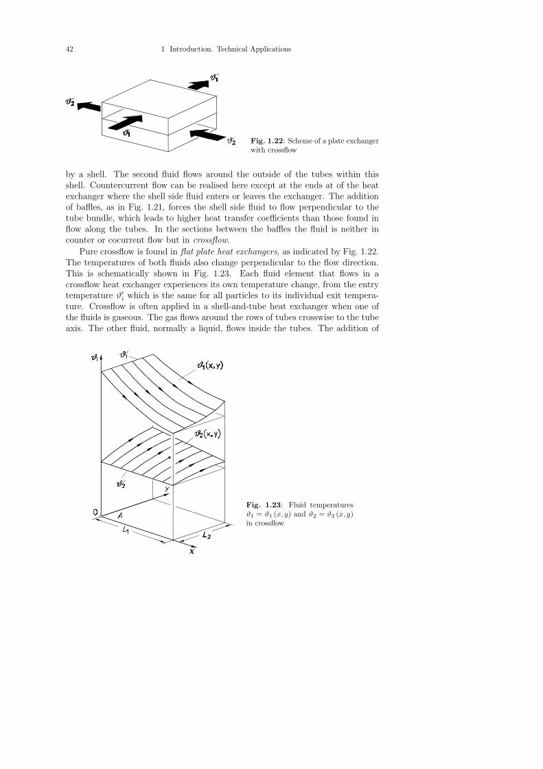
Fig. 1.22: Scheme of a plate exchangerwith crossflow

by a shell. The second fluid flows around the outside of the tubes within thisshell. Countercurrent flow can be realised here except at the ends at of the heatexchanger where the shell side fluid enters or leaves the exchanger. The additionof baffles, as in Fig. 1.21, forces the shell side fluid to flow perpendicular to thetube bundle, which leads to higher heat transfer coefficients than those found inflow along the tubes. In the sections between the baffles the fluid is neither incounter or cocurrent flow but in crossflow.

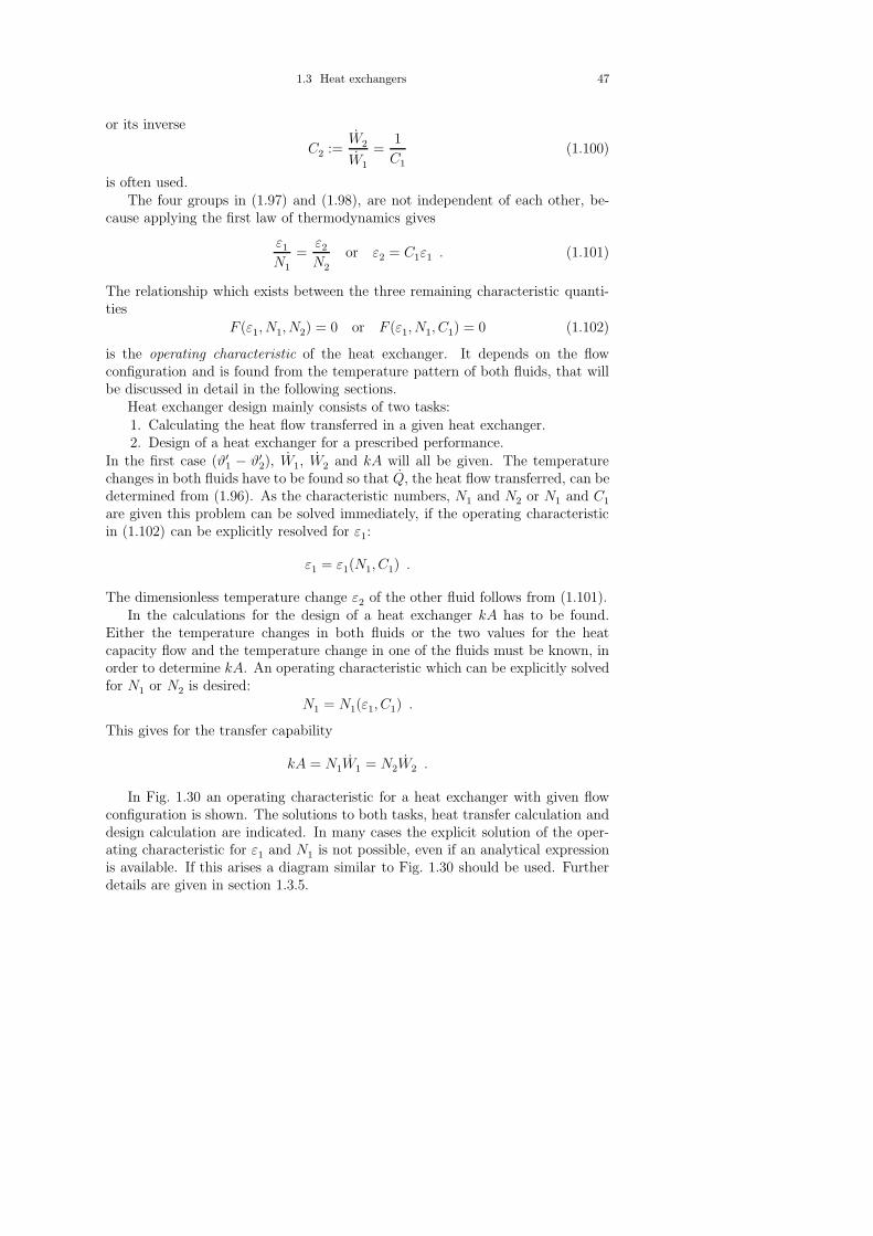
Pure crossflow is found in flat plate heat exchangers, as indicated by Fig. 1.22.The temperatures of both fluids also change perpendicular to the flow direction.This is schematically shown in Fig. 1.23. Each fluid element that flows in acrossflow heat exchanger experiences its own temperature change, from the entrytemperature ϑ′

i which is the same for all particles to its individual exit tempera-ture. Crossflow is often applied in a shell-and-tube heat exchanger when one ofthe fluids is gaseous. The gas flows around the rows of tubes crosswise to the tubeaxis. The other fluid, normally a liquid, flows inside the tubes. The addition of

Fig. 1.23: Fluid temperaturesϑ1 = ϑ1 (x, y) and ϑ2 = ϑ2 (x, y)in crossflow


Fig. 1.24: Coiled tube heatexchanger (schematic)

Fig. 1.25: Regenerators forthe periodic heat transfer be-tween the gases, air and nitro-gen (schematic)

fins to the outer tube walls, cf. 1.2.3 and 2.2.3, increases the area available forheat transfer on the gas side, thereby compensating for the lower heat transfercoefficient.

Fig. 1.24 shows a particularly simple heat exchanger design, a coiled tube insidea vessel, for example a boiler. One fluid flows through the tube, the other one isin the vessel and can either flow through the vessel or stay there while it is beingheated up or cooled down. The vessel is usually equipped with a stirrer that mixesthe fluid, improving the heat transfer to the coiled tube.

There are also numerous other special designs for heat exchangers which willnot be discussed here. It is possible to combine the three basic flow regimes ofcountercurrent, cocurrent and crossflow in a number of different ways, which leadsto complex calculation procedures.


The heat exchangers dealt with so far have had two fluids flowing steadily through theapparatus at the same time. They are always separated by a wall through which heat flows fromthe hotter to the colder fluid. These types of heat exchangers are also known as recuperators,which are different from regenerators. They contain a packing material, for example a lattice ofbricks with channels for the gas or a packed bed of stone or metal strips, that will allow gases topass through it. The gases flow alternately through the regenerator. The hot gas transfers heatto the packing material, where it is stored as internal energy. Then the cold gas flows throughthe regenerator, removes heat from the packing and leaves at a higher temperature. Continuousoperation requires at least two regenerators, so that one gas can be heated whilst the other oneis being cooled, Fig. 1.25. Each of the regenerators will be periodically heated and cooled byswitching the gas flows around. This produces a periodic change in the exit temperatures of thegases.

Regenerators are used as air preheaters in blast furnaces and as heat exchangers in lowtemperature gas liquefaction plants. A special design, the Ljungstrom preheater, equipped witha rotating packing material serves as a preheater for air in firing equipment and gas turbineplants.The warm gas in this case is the exhaust gas from combustion which should be cooled asmuch as possible for energy recovery.

The regenerator theory was mainly developed by H. Hausen [1.10]. As it includes a number ofcomplicated calculations of processes that are time dependent no further study of the theory willbe made here. The summary by H. Hausen [1.7] and the VDI-Warmeatlas [1.11] are suggestedfor further study on this topic.

1.3.2 General design equations. Dimensionless groups

Fig. 1.26 is a scheme for a heat exchanger. The temperatures of the two fluids aredenoted by ϑ1 and ϑ2, as in section 1.3.1, and it will be assumed that ϑ1 > ϑ2.Heat will therefore be transferred from fluid 1 to fluid 2. Entry temperatures areindicated by one dash, exit temperatures by two dashes.

The first law of thermodynamics is applied to for both fluids. The heat trans-ferred causes an enthalpy increase in the cold fluid 2 and a decrease in the warmfluid 1. This gives

Q = M1(h′1 − h′′1) = M2(h

′′2 − h′2) , (1.93)

where Mi is the mass flow rate of fluid i. The specific enthalpies are calculated

Fig. 1.26: Heat exchanger scheme, with the massflow rate Mi, entry temperatures ϑ′

i, exit temper-atures ϑ′′i , entry enthalpy h′i and exit enthalpy h′′iof both fluids (i = 1, 2)


at the entry and exit temperatures ϑ′i and ϑ′′

i respectively. These temperaturesare averaged over the relevant tube cross section, and can be determined usingthe explanation in section 1.1.3 for calculating adiabatic mixing temperatures.Equation (1.93) is only valid for heat exchangers which are adiabatic with respectto their environment, and this will always be assumed to be the case.

The two fluids flow through the heat exchanger without undergoing a phasechange, i.e. they do not boil or condense. The small change in specific enthalpywith pressure is neglected. Therefore only the temperature dependence is impor-tant, and with

cpi :=h′i − h′′iϑ′

i − ϑ′′i

, i = 1, 2 (1.94)

the mean specific heat capacity between ϑ′i and ϑ′′

i it follows from (1.93) that

Q = M1cp1(ϑ′1 − ϑ′′

1) = M2cp2(ϑ′′2 − ϑ′

2) .

As an abbreviation the heat capacity flow rate is introduced by

Wi := Micpi , i = 1, 2 (1.95)

which then givesQ = W1(ϑ

′1 − ϑ′′

1) = W2(ϑ′′2 − ϑ′

2) . (1.96)

The temperature changes in both fluids are linked to each other due to the first lawof thermodynamics. They are related inversely to the ratio of the heat capacityflow rates.

The heat flow Q is transferred from fluid 1 to fluid 2 because of the temperaturedifference ϑ1−ϑ2 inside the heat exchanger. This means that the heat flow Q has toovercome the overall resistance to heat transfer 1/kA according to section 1.2.1.The quantity kA will from now on be called the transfer capability of the heatexchanger, and is a characteristic quantity of the apparatus. It is calculated using(1.72) from the transfer resistances in the fluids and the resistance to conductionin the wall between them. The value for kA is usually taken to be an apparatusconstant, where the overall heat transfer coefficient k is assumed to have the samevalue throughout the heat exchanger. However this may not always happen, thefluid heat transfer coefficient can change due to the temperature dependence ofsome of the fluid properties or by a variation in the flow conditions. In cases suchas these, k and kA must be calculated for various points in the heat exchangerand a suitable mean value can be found, cf. W. Roetzel and B. Spang [1.12], torepresent the characteristic transfer capability kA of the heat exchanger.

Before beginning calculations for heat exchanger design, it is useful to getan overview of the quantities which have an effect on them. Then the numberof these quantities will be reduced by the introduction of dimensionless groups.Finally the relevant relationships for the design will be determined. Fig. 1.27contains the seven quantities that influence the design of a heat exchanger. Theeffectiveness of the heat exchanger is characterised by its transfer capability kA,


Fig. 1.27: Heat exchanger with theseven quantities which affect its design

Fig. 1.28: The three decisivetemperature differences (ar-rows) in a heat exchanger

the two fluid flows by their heat capacity flow rates Wi, entry temperatures ϑ′i and

exit temperatures ϑ′′i . As the temperature level is not important only the three

temperature differences (ϑ′1 − ϑ′′

1), (ϑ′′2 − ϑ′

2) and (ϑ′1 − ϑ′

2), as shown in Fig. 1.28,are of influence. This reduces the number of quantities that have any effect byone so that six quantities remain:

kA, (ϑ′1 − ϑ′′

1), W1, (ϑ′′2 − ϑ′

2), W2 and (ϑ′1 − ϑ′

2) .

These belong to only two types of quantity either temperature (unit K) or heatcapacity flow rate (units W/K). According to section 1.1.4, that leaves four (= 6−2) characteristic quantities to be defined. These are the dimensionless temperaturechanges in both fluids

ε1 :=ϑ′

1 − ϑ′′1

ϑ′1 − ϑ′

2

and ε2 :=ϑ′′

2 − ϑ′2

ϑ′1 − ϑ′

2

, (1.97)

see Fig. 1.29, and the ratios

N1 :=kA

W1

and N2 :=kA

W2

. (1.98)

These are also known as the Number of Transfer Units or NTU for short. Wesuggest Ni be characterised as the dimensionless transfer capability of the heatexchanger. Instead of N2 the ratio of the two heat capacity flow rates

C1 :=W1

W2

=N2

N1

(1.99)

Fig. 1.29: Plot of the dimensionless fluid tempera-tures ϑ+

i = (ϑi − ϑ′2) / (ϑ′1 − ϑ′2) over the area and il-lustration of ε1 and ε2 according to (1.97)


or its inverse

C2 :=W2

W1

=1

C1

(1.100)

is often used.The four groups in (1.97) and (1.98), are not independent of each other, be-

cause applying the first law of thermodynamics gives

ε1

N1

=ε2

N2

or ε2 = C1ε1 . (1.101)

The relationship which exists between the three remaining characteristic quanti-ties

F (ε1, N1, N2) = 0 or F (ε1, N1, C1) = 0 (1.102)

is the operating characteristic of the heat exchanger. It depends on the flowconfiguration and is found from the temperature pattern of both fluids, that willbe discussed in detail in the following sections.

Heat exchanger design mainly consists of two tasks:1. Calculating the heat flow transferred in a given heat exchanger.2. Design of a heat exchanger for a prescribed performance.

In the first case (ϑ′1 − ϑ′

2), W1, W2 and kA will all be given. The temperaturechanges in both fluids have to be found so that Q, the heat flow transferred, can bedetermined from (1.96). As the characteristic numbers, N1 and N2 or N1 and C1

are given this problem can be solved immediately, if the operating characteristicin (1.102) can be explicitly resolved for ε1:

ε1 = ε1(N1, C1) .

The dimensionless temperature change ε2 of the other fluid follows from (1.101).In the calculations for the design of a heat exchanger kA has to be found.

Either the temperature changes in both fluids or the two values for the heatcapacity flow and the temperature change in one of the fluids must be known, inorder to determine kA. An operating characteristic which can be explicitly solvedfor N1 or N2 is desired:

N1 = N1(ε1, C1) .

This gives for the transfer capability

kA = N1W1 = N2W2 .

In Fig. 1.30 an operating characteristic for a heat exchanger with given flowconfiguration is shown. The solutions to both tasks, heat transfer calculation anddesign calculation are indicated. In many cases the explicit solution of the oper-ating characteristic for ε1 and N1 is not possible, even if an analytical expressionis available. If this arises a diagram similar to Fig. 1.30 should be used. Furtherdetails are given in section 1.3.5.


Fig. 1.30: Schematic representation of the operating characteristic for a heat ex-changer with Ci = const. N is the assumed operating point for the heat trans-fer calculations: εi = εi (Ni, Ci), A is the assumed operating point for the design:Ni = Ni (εi, Ci). The determination of the mean temperature difference Θ for pointA is also shown.

When the heat capacity flow rate Wi was introduced in (1.95) boiling and con-densing fluids were not considered. At constant pressure a pure substance whichis boiling or condensing does not undergo a change in temperature, but cpi → ∞.

This leads to εi = 0, whilst Wi → ∞ resulting in Ni = 0 and Ci → ∞. Thissimplifies the calculations for the heat exchanger, as the operating characteristicis now a relationship between only two rather than three quantities, namely ε andN of the other fluid, which is neither boiling nor condensing.

In heat exchanger calculations another quantity alongside those already introduced is oftenused, namely the mean temperature difference ∆ϑm. This is found by integrating the localtemperature difference (ϑ1 − ϑ2) between the two fluids over the whole transfer area.

∆ϑm =1

A

∫

(A)

(ϑ1 − ϑ2) dA . (1.103)

In analogy to (1.71) the heat flow transferred is

Q = kA∆ϑm . (1.104)

This equation can only strictly be used if the heat transfer coefficient k is the same at each pointon A. If this is not true then (1.104) can be considered to be a definition for a mean value of k.

The introduction of ∆ϑm in conjunction with (1.104), gives a relationship between theheat flow transferred and the transfer capability kA, and therefore with the area A of the heatexchanger. This produces the following equations

Q = kA∆ϑm = W1(ϑ′

1 − ϑ′′1) = W2(ϑ′′

2 − ϑ′2) .

With the dimensionless mean temperature difference

Θ =∆ϑm

ϑ′1 − ϑ′2(1.105)

the following relationship between the dimensionless groups is found:

Θ =ε1N1

=ε2N2

. (1.106)


The mean temperature ∆ϑm and its associated dimensionless quantity Θ can be calculatedusing the dimensionless numbers that have already been discussed. The introduction of themean temperature difference does not provide any information that cannot be found from theoperating characteristic. This is also illustrated in Fig. 1.30, where Θ is the gradient of thestraight line that joins the operating point and the origin of the graph.

1.3.3 Countercurrent and cocurrent heat exchangers

The operating characteristic F (εi, Ni, Ci) = 0, for a countercurrent heat exchangeris found by analysing the temperature distribution in both fluids. The results caneasily be transferred for use with the practically less important case of a cocurrentexchanger.

We will consider the temperature changes, shown in Fig. 1.31, in a countercur-rent heat exchanger. The temperatures ϑ1 and ϑ2 depend on the z coordinate inthe direction of flow of fluid 1. By applying the first law to a section of length dzthe rate of heat transfer, dQ, from fluid 1 to fluid 2 through the surface elementdA is found to be

dQ = −M1cp1 dϑ1 = −W1 dϑ1 (1.107)

anddQ = −M2cp2 dϑ2 = −W2 dϑ2 . (1.108)

Now dQ is eliminated by using the equation for overall heat transfer

dQ = k (ϑ1 − ϑ2) dA = kA (ϑ1 − ϑ2)dz

L(1.109)

from (1.107) and (1.108) giving

dϑ1 = −(ϑ1 − ϑ2)kA

W1

dz

L= −(ϑ1 − ϑ2)N1

dz

L(1.110)

Fig. 1.31: Temperature pattern in acountercurrent heat exchanger


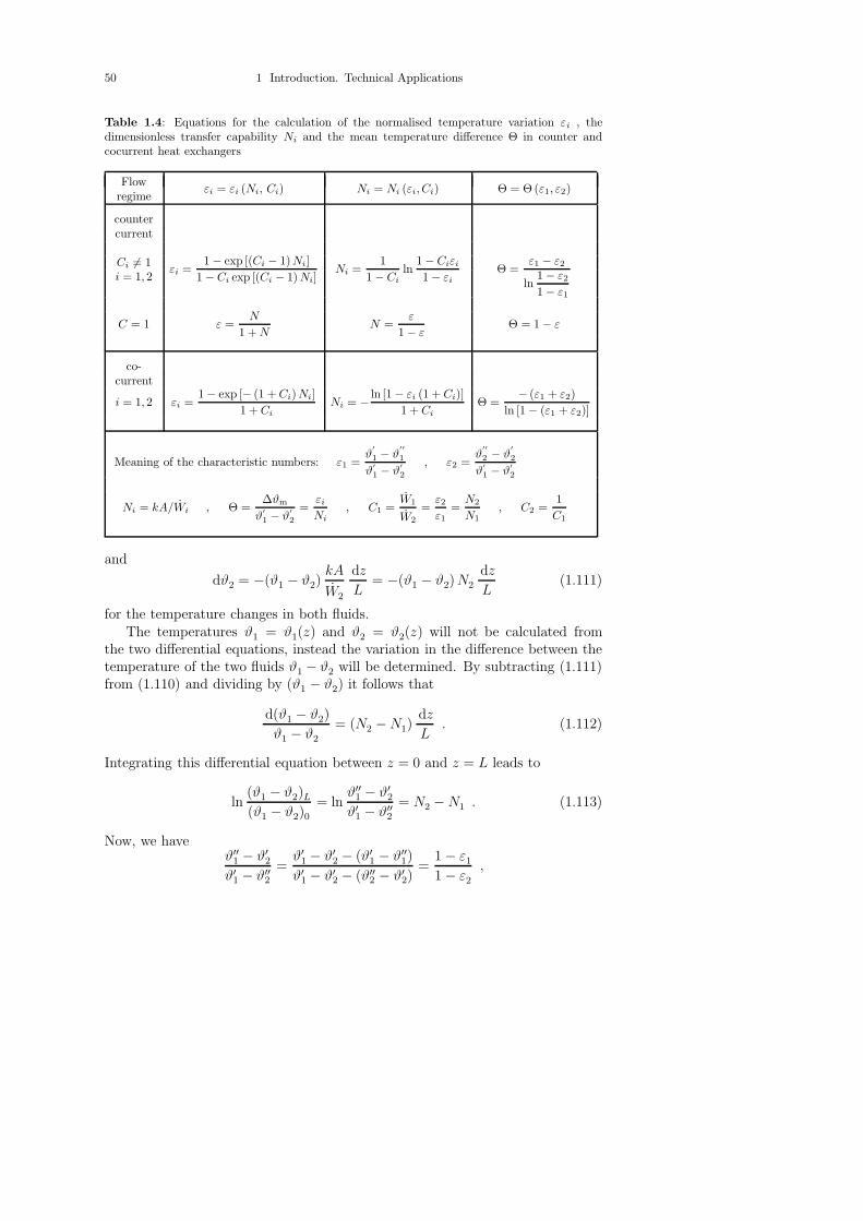
Table 1.4: Equations for the calculation of the normalised temperature variation εi , thedimensionless transfer capability Ni and the mean temperature difference Θ in counter andcocurrent heat exchangers

Flowregime

εi = εi (Ni, Ci) Ni = Ni (εi, Ci) Θ = Θ(ε1, ε2)

countercurrent

Ci 6= 1i = 1, 2

εi =1 − exp [(Ci − 1)Ni]

1 − Ci exp [(Ci − 1)Ni]Ni =

1

1 − Ciln

1 − Ciεi

1 − εiΘ =

ε1 − ε2

ln1 − ε21 − ε1

C = 1 ε =N

1 +NN =

ε

1 − εΘ = 1 − ε

co-current

i = 1, 2 εi =1 − exp [− (1 +Ci)Ni]

1 + CiNi = − ln [1 − εi (1 + Ci)]

1 + CiΘ =

− (ε1 + ε2)

ln [1 − (ε1 + ε2)]

Meaning of the characteristic numbers: ε1 =ϑ

′

1 − ϑ′′

1

ϑ′

1 − ϑ′

2

, ε2 =ϑ

′′

2 − ϑ′

2

ϑ′

1 − ϑ′

2

Ni = kA/Wi , Θ =∆ϑm

ϑ′

1 − ϑ′

2

=εi

Ni, C1 =

W1

W2

=ε2ε1

=N2

N1, C2 =

1

C1

and

dϑ2 = −(ϑ1 − ϑ2)kA

W2

dz

L= −(ϑ1 − ϑ2)N2

dz

L(1.111)

for the temperature changes in both fluids.The temperatures ϑ1 = ϑ1(z) and ϑ2 = ϑ2(z) will not be calculated from

the two differential equations, instead the variation in the difference between thetemperature of the two fluids ϑ1 − ϑ2 will be determined. By subtracting (1.111)from (1.110) and dividing by (ϑ1 − ϑ2) it follows that

d(ϑ1 − ϑ2)

ϑ1 − ϑ2

= (N2 −N1)dz

L. (1.112)

Integrating this differential equation between z = 0 and z = L leads to

ln(ϑ1 − ϑ2)L

(ϑ1 − ϑ2)0= ln

ϑ′′1 − ϑ′

2

ϑ′1 − ϑ′′

2

= N2 −N1 . (1.113)

Now, we haveϑ′′

1 − ϑ′2

ϑ′1 − ϑ′′

2

=ϑ′

1 − ϑ′2 − (ϑ′

1 − ϑ′′1)

ϑ′1 − ϑ′

2 − (ϑ′′2 − ϑ′

2)=

1 − ε1

1 − ε2

,


Fig. 1.32: Operating characteristic εi = εi (Ni, Ci) for countercurrent flow from Tab. 1.4

which gives

ln1 − ε1

1 − ε2

= N2 −N1 (1.114)

as the implicit form of the operating characteristic of a countercurrent heat ex-changer. It is invariant with respect to an exchange of the indices 1 and 2. Usingthe ratios of C1 and C2 = 1/C1 from (1.99) and (1.100), explicit equations areobtained,

εi = f(Ni, Ci) and Ni = f(εi, Ci) , i = 1, 2

which have the same form for both fluids. These explicit formulae for the operatingcharacteristics are shown in Table 1.4. If the heat capacity flow rates are equal,W1 = W2, and because C1 = C2 = 1, it follows that

ε1 = ε2 = ε and N1 = N2 = N ,

and with a series development of the equations valid for Ci 6= 1 towards the limitof Ci → 1, the simple relationships given in Table 1.4 are obtained.

Fig. 1.32 shows the operating characteristic εi = f(Ni, Ci) as a function of Ni

with Ci as a parameter. As expected the normalised temperature change εi growsmonotonically with increasing Ni, and therefore increasing transfer capability kA.For Ni → ∞ the limiting value is

limNi→∞

εi =

{1 for Ci ≤ 1

1/Ci for Ci > 1.

If Ci ≤ 1, then εi takes on the character of an efficiency. The normalised tem-perature change of the fluid with the smaller heat capacity flow is known as theefficiency or effectiveness of the heat exchanger. With an enlargement of the heattransfer area A the temperature difference between the two fluids can be made assmall as desired, but only at one end of the countercurrent exchanger. Only for


W1 = W2, which means C1 = C2 = 1, can an infinitely small temperature differ-ence at at both ends, and therefore throughout the heat exchanger, be achievedby an enlargement of the surface area. The ideal case of reversible heat transferbetween two fluids, often considered in thermodynamics, is thus only attainablewhen W1 = W2 in a heat exchanger with very high transfer capability.

As already mentioned in section 1.3.2, the function εi = f(Ni, Ci) is usedto calculate the outlet temperature and the transfer capability of a given heatexchanger. For the sizing of a heat exchanger for a required temperature changein the fluid, the other form of the operating characteristic, Ni = Ni(εi, Ci), isused. This is also given in Table 1.4.

In a cocurrent heat exchanger the direction of flow is opposite to that in Fig.1.31, cf. also Fig. 1.20b. In place of (1.108) the energy balance is

dQ = M2cp2 dϑ2 = W2 dϑ2 ,

which gives the relationship

d(ϑ1 − ϑ2)

ϑ1 − ϑ2

= −(N1 +N2)dz

L(1.115)

instead of (1.112). According to (1.114) the temperature difference between thetwo fluids in the direction of flow is always decreasing. Integration of (1.115)between z = 0 and z = L yields

lnϑ′′

1 − ϑ′′2

ϑ′1 − ϑ′

2

= −(N1 +N2) ,

from which follows

ln [1 − (ε1 + ε2)] = −(N1 +N2) = −ε1 + ε2

Θ(1.116)

as the implicit form of the operating characteristic. This can be solved for εi

and Ni giving the functions noted in Table 1.4. For Ni → ∞ the normalisedtemperature variation reaches the limiting value of

limNi→∞

εi =1

1 + Ci

, i = 1, 2 .

With cocurrent flow the limiting value of εi = 1 is never reached except whenCi = 0, as will soon be explained.

The calculations for performance and sizing of a heat exchanger can also be carried outusing a mean temperature difference Θ from (1.105) in section 1.3.2. In countercurrent flow, thedifference N2 − N1 in (1.113) is replaced by Θ, ε1 and ε2 giving the expression Θ = Θ(ε1, ε2)which appears in Table 1.4. Introducing

N2 −N1 =ε2 − ε1

Θ=ϑ′′2 − ϑ′2 − (ϑ′1 − ϑ′′1)

∆ϑm=ϑ′′1 − ϑ′2 − (ϑ′1 − ϑ′′2)

∆ϑm


Fig. 1.33: Temperature in a condenser with cooling of superheated steam,condensation and subcooling of the condensate (fluid 1) by cooling water(fluid 2)

into (1.113) , gives

∆ϑm =ϑ′′1 − ϑ′2 − (ϑ′1 − ϑ′′2)

lnϑ′′1 − ϑ′2ϑ′1 − ϑ′′2

(1.117)

for the mean temperature difference in a countercurrent heat exchanger. It is the logarithmic

mean of the temperature difference between the two fluids at both ends of the apparatus.The expression, from (1.116), for the normalised mean temperature difference Θ, in cocur-

rent flow is given in Table 1.4. Putting in (1.117) the defining equations for ε1 and ε2 yields

∆ϑm =ϑ′1 − ϑ′2 − (ϑ′′1 − ϑ′′2)

lnϑ′1 − ϑ′2ϑ′′1 − ϑ′′2

. (1.118)

So ∆ϑm is also the logarithmic mean temperature difference at both ends of the heat exchangerin cocurrent flow.

We will now compare the two flow configurations. For Ci = 0 the normalisedtemperature variation in Table 1.4 is

εi = 1 − exp(−Ni)

and the dimensionless transfer capability

Ni = − ln(1 − εi)

both of which are independent of whether countercurrent or cocurrent flow isused. Therefore when one of the substances boils or condenses in the exchangerit is immaterial which flow configuration is chosen. However, if in a condenser,superheated steam is first cooled from ϑ′

1 to the condensation temperature ofϑ1s, then completely condensed, after which the condensate is cooled from ϑ1s

to ϑ′′1, more complex circumstances develop. In these cases it is not permissible

to treat the equipment as simply one heat exchanger, using the equations thathave already been defined, where only the inlet and outlet temperatures ϑ′

i and


Fig. 1.34: Ratio (kA)co / (kA)cc = N coi /N cc

i of the transfer capabilities in cocur-rent (index co) and countercurrent (index cc) flows as a function of εi and Ci

ϑ′′i (i = 1, 2) are important, cf. Fig. 1.33. The values for the heat capacity flow

rate W1 change significantly: During the cooling of the steam and the condensateW1 has a finite value, whereas in the process of condensation W1 is infinite. Theexchanger has to be imaginarily split, and then be treated as three units in series.Energy balances provide the two unknown temperatures, ϑ2a between the coolingand condensation section, and ϑ2b, between the condensation and sub-coolingpart. These in turn yield the dimensionless temperature differences εia, εib andεic for the three sections cooler a, condenser b and sub-cooler c (i = 1, 2). Thedimensionless transfer capabilities Nia, Nib and Nic of the three equipment sectionscan then be calculated according to the relationships in Table 1.4. From Nij thevalues for (kA)j can be found. Then using the relevant overall heat transfercoefficients kj, we obtain the areas of the three sections Aj (j = a, b, c), whichtogether make up the total transfer area of the exchanger.

For Ci > 0 the countercurrent configuration is always superior to the cocurrent.A disadvantage of the cocurrent flow exists in that not all heat transfer tasks canbe solved in such a system. A given temperature change εi is only realisable ifthe argument of the logarithmic term in

N coi = − 1

1 + Ci

ln [1 − εi(1 + Ci)]

is positive. This is only the case for

εi <1

1 + Ci

. (1.119)

Larger normalised temperature changes cannot be achieved in cocurrent heat ex-changers even in those with very large values for the transfer capability kA. Incountercurrent exchangers this limitation does not exist. All values for εi are ba-sically attainable and therefore all required heat loads can be transferred as longas the area available for heat transfer is made large enough.


A further disadvantage of cocurrent flow is that a higher transfer capabilitykA is required to fulfill the same task (same εi and Ci) when compared with acountercurrent system. This is shown in Fig. 1.34 in which the ratio

(kA)co/(kA)cc = N coi /N

cci

based on the equations in Table 1.4 is represented. This ratio grows sharply whenεi approaches the limiting value according to (1.119). Even when a cocurrentexchanger is capable of fulfilling the requirements of the task, the countercurrentexchanger will be chosen as its dimensions are smaller. Only in a combination ofsmall enough values of Ci and εi the necessary increase in the area of a cocurrentexchanger is kept within narrow limits.

Example 1.4: Ammonia, at a pressure of 1.40 MPa, is to be cooled in a countercurrentheat exchanger from ϑ′

1 = 150.0 ◦C to the saturation temperature ϑ′

1s = 36.3 ◦C, andthen completely condensed. Its mass flow rate is M1 = 0.200 kg/s. Specific enthalpies ofh(ϑ′1) = 1797.1 kJ/kg, hg(ϑ1s) = 1488.8 kJ/kg, and hfl(ϑ1s) = 372.2 kJ/kg are taken fromthe property tables for ammonia, [1.13]. Cooling water with a temperature of ϑ′

2 = 12.0 ◦Cis available, and this can be heated to ϑ′′

2 = 28.5 ◦C. Its mean specific heat capacity iscp2 = 4.184 kJ/kgK. The required transfer capabilities for the cooling (kA)cooling and(kA)cond for the condensation of the ammonia have to be determined.At first the heat flow transferred Q, and the required mass flow rate M2 of water have tobe found. The heat flow removed from the ammonia is

Q = M1

[h(ϑ′1) − hfl(ϑ1s)

]= 0.200

kg

s(1797.1 − 372.2)

kJ

kg= 285.0 kW .

From that the mass flow rate of water is found to be

M2 =Q

cp2 (ϑ′′2 − ϑ′1)=

285.0 kW

4.184 (kJ/kgK) (28.5 − 12.0) K= 4.128

kg

s.

The temperature ϑ2a of the cooling water in the cross section between the cooling andcondensation sections, cf. Fig. 1.35, is required to calculate the transfer capability.

Fig. 1.35: Temperatures ofammonia and cooling waterin a countercurrent heat ex-changer (schematic)

From the energy balance for the condensor section

M2cp2 (ϑa − ϑ′2) = M1

[hg(ϑ1s) − hfl(ϑ1s)

],

it follows that

ϑ2a = ϑ′2 +M1

M2cp2

[hg(ϑ1s) − hfl(ϑ1s)

]= 24.9 ◦C .


The transfer capability for the ammonia cooling section, using Table 1.4, is

(kA)cooling

W1

= N1 =1

1 − C1ln

1 − C1ε11 − ε1

. (1.120)

The ratio of the heat capacity flow rates is found with

W1 = M1cp1 = M1h(ϑ′1) − hg(ϑs)

ϑ′1 − ϑs= 0.200

kg

s

1797.1 − 1488.8

150.0 − 36.3

kJ

kgK= 0.5423

kW

K

and with W2 = M2cp2 = 17.272 kW/K giving C1 = 0.0314. The dimensionless temperaturevariation of ammonia is

ε1 =ϑ′1 − ϑs

ϑ′1 − ϑ2a=

150.0 − 36.3

150.0 − 24.9= 0.9089.

Then (1.120) yields N1 = 2.443 and finally

(kA)cooling = N1W1 = 1.325 kW/K .

For the condensation section of the heat exchanger ε1 = 0, and because W1 → ∞ thismeans C2 = W2/W1 = 0. From Table 1.4 it follows that

(kA)cond/W2 = N2 = − ln (1 − ε2) .

With the normalised temperature change of the cooling water

ε2 =ϑ2a − ϑ′2ϑ1s − ϑ′2

=24.9 − 12.0

36.3 − 12.0= 0.5309 ,

yielding N2 = 0.7569, which then gives

(kA)cond = N2W2 = 13.07 kW/K .

In order to find the required area A = Acooling + Acond for the countercurrent exchanger,from the values for (kA)cooling and (kA)cond, the overall heat transfer coefficients for eachpart must be calculated. They will be different as the resistance to heat transfer in thecooling section is greatest on the gaseous ammonia side, whereas in the condensationsection the greatest resistance to heat transfer is experienced on the cooling water side.The calculations for the overall heat transfer coefficients will not be done here as the designof the heat exchanger and the flow conditions have to be known for this purpose.

1.3.4 Crossflow heat exchangers

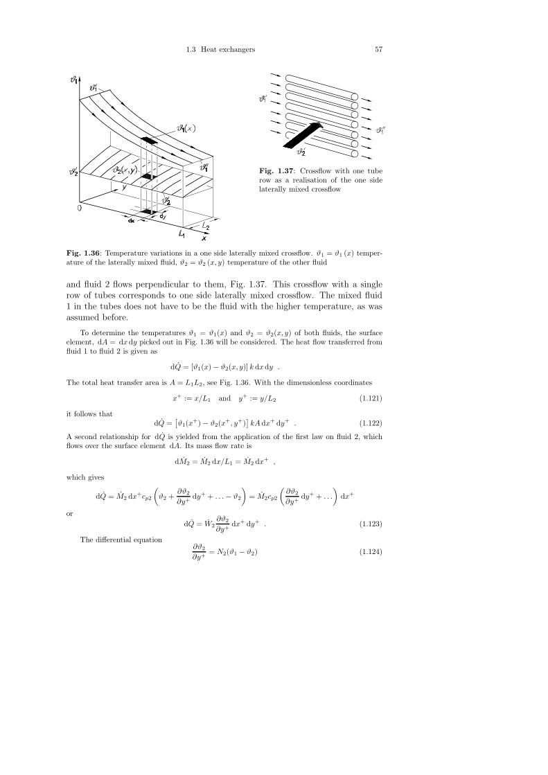
Before discussing pure crossflow as shown in Fig. 1.23, the operating characteristicfor the simple case of crossflow where only the fluid on one side is laterally mixedwill be calculated. In this flow configuration the temperature of one of the twofluids is only dependent on one position coordinate, e.g. x, while the temperatureof the other fluid changes with both x and y. In Fig. 1.36 the laterally mixed fluidis indicated by the index 1. Its temperature ϑ1 changes only in the direction offlow, ϑ1 = ϑ1(x). Ideal lateral mixing is assumed so that ϑ1does not vary with y.This assumption is closely met when fluid 1 flows through a single row of tubes


Fig. 1.37: Crossflow with one tuberow as a realisation of the one sidelaterally mixed crossflow

Fig. 1.36: Temperature variations in a one side laterally mixed crossflow. ϑ1 = ϑ1 (x) temper-ature of the laterally mixed fluid, ϑ2 = ϑ2 (x, y) temperature of the other fluid

and fluid 2 flows perpendicular to them, Fig. 1.37. This crossflow with a singlerow of tubes corresponds to one side laterally mixed crossflow. The mixed fluid1 in the tubes does not have to be the fluid with the higher temperature, as wasassumed before.

To determine the temperatures ϑ1 = ϑ1(x) and ϑ2 = ϑ2(x, y) of both fluids, the surfaceelement, dA = dxdy picked out in Fig. 1.36 will be considered. The heat flow transferred fromfluid 1 to fluid 2 is given as

dQ = [ϑ1(x) − ϑ2(x, y)] k dxdy .

The total heat transfer area is A = L1L2, see Fig. 1.36. With the dimensionless coordinates

x+ := x/L1 and y+ := y/L2 (1.121)

it follows thatdQ =

[ϑ1(x

+) − ϑ2(x+, y+)

]kAdx+ dy+ . (1.122)

A second relationship for dQ is yielded from the application of the first law on fluid 2, whichflows over the surface element dA. Its mass flow rate is

dM2 = M2 dx/L1 = M2 dx+ ,

which gives

dQ = M2 dx+cp2

(ϑ2 +

∂ϑ2

∂y+dy+ + . . .− ϑ2

)= M2cp2

(∂ϑ2

∂y+dy+ + . . .

)dx+

or

dQ = W2∂ϑ2

∂y+dx+ dy+ . (1.123)

The differential equation∂ϑ2

∂y+= N2(ϑ1 − ϑ2) (1.124)

http://www.springer.com/978-3-540-29526-6

1.3 heat exchangers - springer

Documents