13 Trapping and Cooling

Whereas first single atom experiments exploited dilute atomic beams, modern ap-proaches investigate trapped atoms. One distinguishes between traps for chargedatoms, i.e. ions and traps for neutral atoms.

13.1 Ion traps

13.1.1 Paul traps

It is well known from the so-called Earnshaw theorem that a charged particle cannotbe trapped in a stable configuration with static electric fields only. However, a com-bination of static electric and magnetic fields (Penning trap) or time dependentelectric fields (Paul trap) can provide space points where a restoring force in allthree directions acts on a charged particle.

A Paul trap (Nobel Prize 1989) consists of two parabolical electrodes and a ringelectrode.

Figure 105: Sketch of a Paul trap

183

Figure 106: Photo of a Paul trap [from http://www.physik.uni-mainz.de]

If a dc-voltage Udc and an ac-voltage Vac of frequency Ω is applied to the electrodesthen the potential near the trap axis is of the form:

Φ =(Udc + Vac cos(Ωt))(r2 − 2z2 + 2z2

0)

r20 + 2z2

0

where r0 and z0 denote the distances from the trap axis to the surface of the elec-trodes.

The potential is harmonic and for a certain time t provides a restoring force inone dimension.

Say, at a given time t the x-direction is the non-confining direction. Then, due toits inertia a particle cannot escape along that direction before the sign of cos(Ωt) isinverted, and the x-direction becomes the confining direction. For certain frequen-cies Ω this results in an effective confinement in all three directions.

184

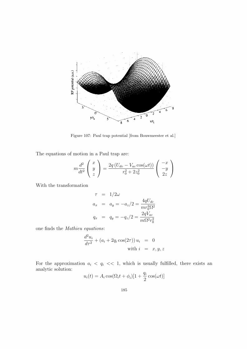
Figure 107: Paul trap potential [from Bouwmeester et al.]

The equations of motion in a Paul trap are:

md2

dt2

xyz

=

2q (Udv − Vac cos(ωt))

r20 + 2z2

0

−x−y2z

With the transformation

τ = 1/2ω

ax = ay = −az/2 =4qUdc

mr20Ω

2

qx = qy = −qz/2 =2qVac

mΩ2r20

one finds the Mathieu equations :

d2ui

dτ 2+ (ai + 2qi cos(2τ)) ui = 0

with i = x, y, z

For the approximation ai < qi << 1, which is usually fulfilled, there exists ananalytic solution:

ui(t) = Ai cos(Ωit + φi)[1 +qi

2cos(ωt)]

185

The solution consist of a rapid oscillation with the trap frequency ω, the so-calledmicromotion, and a slower macromotion (or secular motion) at frequency Ωi in theeffective harmonic trap potential with:

Ωi ≈ ω

2(ai +

qi

2)

In the trap center the micromotion vanishes completely.

As an example of a very fundamental experiment with single trapped ions Fig. 109shows the fluorescence from a single Ba-Ion.

Figure 108: Energy levels of Ba

If a single ion is trapped and continuously illuminated with laser light (here onthe P1/2 −→ S1/2 transition, see Fig. refBalevels) then the fluorescence vanishesabruptly due to transitions to the metastable D5/2 level (The other arrow indicatesrepumping from the D3/2 level). First experiments were performed in 1986. Thepossibility to observe these ”Quantum Jumps” led to many theoretical discussionsin the early 50’s.

13.1.2 Trapping ion strings

In order to realize well-controllable experiments several ions the Paul trap has to bemodified to Linear ion traps. These traps usually consist of two pairs of electrodes(hyperbolically shaped, spherical rods, or rectangular shapes) which provide a con-finement in two directions. These configurations resemble mass spectrometers (moreprecisely e/m filters). A second pair of end cap electrodes provides the confinementin the orthogonal direction. Figure 110 shows various configurations.

186

Figure 109: Quantum jumps of a single Ba-atom[from http://www.physnet.uni-hamburg.de/ilp/toschek/ionen.html]

In a linear trap the equation of motion in z-direction (direction of the end caps)is given by:

d2uz

dt2+ (2κqUcap/mz2

0)uz = 0

where q, m are the charge and mass of the ion and κ is an empirically found param-eter.The equation of motion in the orthogonal directions is given again by the Mathieuequations:

d2ui

dτ 2+ (ai + 2qi cos(2τ)) ui = 0

with i = x, y

187

Figure 110: Different types of linear ion traps [from Bouwmeester et al.]

where

ax =4q

mΩ2

(Udc

r20

− κUcap

z20

)

ay = − 4q

mΩ2

(Udc

r20

+κUcap

z20

)

qx = −qy =2qVac

mΩ2r20

τ = Ωt/2

Similar as in the single-ion trap the motion of the ions can be approximated as acombination of micro- and macromotion. What is important now is that the micro-motion vanishes completely on the whole trap axis!

Figure111 shows a collection of pictures (raw video data) of stored Ca-ion strings.

188

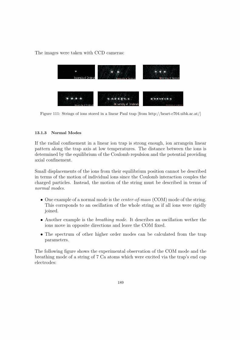
The images were taken with CCD cameras:

Figure 111: Strings of ions stored in a linear Paul trap [from http://heart-c704.uibk.ac.at/]

13.1.3 Normal Modes

If the radial confinement in a linear ion trap is strong enough, ion arrangein linearpattern along the trap axis at low temperatures. The distance between the ions isdetermined by the equilibrium of the Coulomb repulsion and the potential providingaxial confinement.

Small displacements of the ions from their equilibrium position cannot be describedin terms of the motion of individual ions since the Coulomb interaction couples thecharged particles. Instead, the motion of the string must be described in terms ofnormal modes.

• One example of a normal mode is the center-of-mass (COM) mode of the string.This corrsponds to an oscillation of the whole string as if all ions were rigidlyjoined.

• Another example is the breathing mode. It describes an oscillation wether theions move in opposite directions and leave the COM fixed.

• The spectrum of other higher order modes can be calculated from the trapparameters.

The following figure shows the experimental observation of the COM mode and thebreathing mode of a string of 7 Ca atoms which were excited via the trap’s end capelectrodes:

189

Figure 112: Excitation of normal modes in a string of 7 Ca atoms [from Bouwmeester et al.]

190

13.2 Laser Cooling

If a string of trapped ions should be used for quantum computaion it is required tocool ions down to the ground state of their normal modes. (More recent proposalhave weakened this requirement, but cooling is yet desirable).

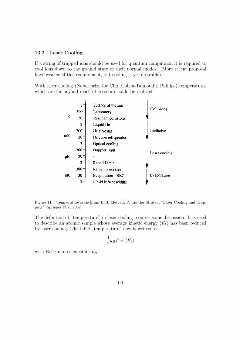
With laser cooling (Nobel prize for Chu, Cohen-Tannoudji, Phillips) temperatureswhich are far beyond reach of cryostats could be realized.

Figure 113: Temperature scale [from H. J. Metcalf, P. van der Straten, ”Laser Cooling and Trap-ping”, Springer N.Y. 2002]

The definition of ”temperature” in laser cooling requires some discussion. It is usedto describe an atomic sample whose average kinetic energy 〈Ek〉 has been reducedby laser cooling. The label ”temperature” now is written as:

1

2kBT = 〈Ek〉

with Boltzmann’s constant kB.

191

13.2.1 Doppler Cooling

The idea of laser cooling is illustrated by the following figure:

Figure 114: Schematics of laser cooling

Assume a moving atom is interacting with monochromatic laser which is red de-tuned from the resonance of an electronic transition of the atom. Then, the atomcan only absorb photons from the laser light if it moves towards the laser and is thustuned to resonance by the Doppler shift. The atom experiences a momentum change∆p which causes a deceleration. After absorption the atom spontaneously emits thephoton again. Since spontaneous emission is isotropic there is no momentum changeon the average. Two laser beams from opposite directions can thus decelerate orcool the atomic motion in one direction. Accordingly, three pairs of laser beamsestablish a cooling in all three directions. The minimum temperature achievable inthis way by Doppler cooling is the Doppler temperature:

kBTD =~Γ2

192

where Γ is the natural linewidth of the transition.

The achievable deceleration is remarkable: An atom moving with a thermal ve-locity of 1000 m/ sec can be stopped within a ms. This correspond roughly to 105

g!

13.2.2 Harmonic potential

As pointed out above the trap potential for ions in a Paul trap is usually harmonicclose to the trap’s center. The Hamiltonian of a particle in a one dimensionalharmonic potential is:

H =p2

2m+

1

2mω2x2

with the definition of the creation and annihilation operator a†, a

a =1√

2m~ω(mωx + ip)

a† =1√

2m~ω(mωx− ip)

with the properties

a† |n〉 =√

n + 1 |n + 1〉a |n〉 =

√n |n− 1〉

one derives the Hamiltonian of the harmonic oscillator:

H = ~ω(

a†a +1

2

)

The motional eigenstates of a trapped particle are thus harmonic oscillator eigen-states with equally spaced eigenvalues and sometimes similar as quantized latticevibrations called phonons. The typical length scale x0 is:

x0 =√~/2mω

13.2.3 Sideband Cooling

In a trap potential ions can be cooled down even further than the Doppler limit bythe so-called sideband cooling. Figure 115 illustrates how this works:

193

Figure 115: Schematics of sideband-cooling [from Bouwmeester et al.]

The lowest picture shows the typical energy structure of an ion in a trap. It is acombination of the ion’s two internal states (e and g) and the motional states. Alaser is tuned to a transition to an excited state with a lower motional excitation.Spontaneous emission now causes a transition without change of the motional state(on the average). Since the potential is harmonic this scheme applies to all pairs ofneighboring motional states. Motional quanta are removed one-by-one in each opti-cal cycle, and the ion ends up in the motional ground state which is then decoupledfrom the laser light.In experimental realizations either a stabilized laser is used to resolve individualsidebands or a Raman transition where the energy difference between two incidentlasers equals the energy of one phonon.

13.2.4 Choosing atoms

Although an ion trap is very deep (several eV potential well depth) and will hold al-most every ion, only a few ions are suitable for quantum computation. The following

194

requirements should be met:

• The electronic level structure should be simple to allow the realization of aclosed two level system without the need of too many lasers.

• The levels used for the qubit transition should have a negligible decoherence(e.g. by spontaneous decay).

• The levels should allow for efficient laser cooling and detection (some strongtransitions).

Because of these requirements the ions of choice have typically only one electron inthe outer shell (hydrogenic ions). The two level system can either be provided bytwo hyperfine ground states or by a ground state and a long-lived metastable elec-tronic state.

Most of the experiments have been done with 9Be+ and 40Ca+, but other possi-ble ions are 138Ba+, 25Mg+, 199Hg+, and 171Y b+.

Figure 116: Energy levels of Ca and Be [from Bouwmeester et al.]

Cooling of the ions starts with Doppler cooling. In 9Be+, the ultraviolet S1/2 −→P3/2 transition at 313 nm is used, while for the 40Ca+ the corresponding transitionis 397 nm. Frequency doubled Ti:Sapphire or dye lasers are used to generate theUV light. (A major advantage of a specific ion could be wether it is possible to usecheap lasers, e.g. diode lasers for the optical excitations!)

The Doppler cooling leads to a thermal state of motion with a temperature of

195

about 1 mK. Then, it depends on the trap depth how many motional states nphonon

are occupied at this temperature. The number ranges between 〈nphonon〉 = 1.3(ωtrap/2π = 11 MHz) and 〈nphonon〉 = 50 (ωtrap/2π = 140 kHz). Subsequent side-band cooling cools the ions to the motional ground state.

13.3 Quantum information gates with trapped ions

13.3.1 Hamiltonian of ions in a trap

The Hamiltonian of N ions in a 3-dimensional harmonic trap potential which interactvia Coulomb interaction is:

HNions =N∑

i=1

m

2

(ωxx

2i + ωyy

2i + ωzz

2i +

|pi|22

)+

N∑i=1

∑i<j

e2

4πε0(−→r i −−→r j)

Since a typical trap potential in a linear ion trap is shallowest in the z-direction (i.e.perdendicular to the end caps) it is sufficient here to consider only the z-coordinate.The ions remain in the ground state with respect to the oscillation in both x- andy-direction.

The ions are laser cooled to the so-called Lamb-Dicke regime. The Lamb-Dickeregime is defined as η ¿ 1, where η is the Lamb-Dicke parameter. This parametergives the ratio between the typical length scale z0 of an ion’s oscillation amplitudein a harmonic trap potential and the wavelength λ of the incident laser radiation:

η = 2πz0/λ = 2π√~/2Nmωtrap/λ

where N is the number of ions in the trap, m the ion’s mass, and ωtrap is the trapfrequency.

If the ions are laser cooled they only perform small oscillations around their equi-librium position. Then the Coulomb potential can be expanded as a Taylor series.Thus, the potential (trap and Coulomb potential) along the z-direction can be writ-ten as:

V (z) =N∑

i=1

N∑j=1

Uijzizj

196

The diagonalization of this potential can be achieved by transforming to the normalvariables. Finally, the Hamiltonian HNions is transformed into

HNions =N∑

i=1

~ωia†iai

which is an harmonic oscillator potential for N normal modes.

13.3.2 Interaction with a laser field

The interaction of the ions in the trap with a classical laser field at frequency ω isnow:

H iI = Ωi cos(kzi + φi + ωt)(σ+

i + σ−i )

Note here that we considered one particular normal mode i and assumed a standingwave laser field. The Rabi-frequency Ωi is proportional to the amplitude of theclassical laser field. σ+

i and σ−i describe the raising and lowering operators of theatom’s two internal states.The coordinate zi is now quantized due to the motion in the trap potential:

zi = zi,equilibrium + 1/√~/2NmωCM(a + a†)

Note: We consider only an excitation of the lowest (center-of-mass) normal mode.

This introduces the factor of 1/√

N to the normal coordinates. With the equilibriumposition absorbed in the phase φi the Hamiltonian reads:

H iI = Ωi cos(

η√N

(a + a†) + φi + ωt)(σ+i + σ−i )

In the limit of small Lamb-Dicke parameter, η ¿ 1, one finds after some algebratwo cases:

1. Laser tuned to the internal atomic transition ω = ω0 :

H iI = Ωi/2

(σ+

i exp(iφi) + σ−i exp(−iφi))

The laser field introduces only transitions between internal states of the ions.

2. Laser tuned to one of the sideband transitions ω = ω0 ± ωCM :

H iI =

Ωi

2√

N

(σ+

i a† exp(iφi)− σ−i a exp(−iφi))

if ω = ω0 + ωCM

H iI =

Ωi

2√

N

(σ+

i a exp(iφi)− σ−i a† exp(−iφi))

if ω = ω0 − ωCM

197

In this case, in addition to an internal transition one phonon is created orannihilated.

The following figure shows a sketch of the different possibilities:

198

Figure 117: Schematics of possible transitions in a trapped ion [from Nielsen and Chuang]

13.3.3 Single qubit operation

A qubit is encoded in the internal states of the ions:

Figure 118: Encoding qubits in a trapped ion [from Bouwmeester et al.]

Single qubit gates are established by tuning the laser to the frequency ω = ω0.By choosing the phase shift φ and the duration of the interaction appropriately,arbitrary rotations can be performed. Thus, any single qubit-gate can be realizedthis way.

199

13.3.4 Two qubit operation

A controlled phase-flip gate can be constructed with the help of an auxiliary atomiclevel in the following way [J. I. Cirac, P. Zoller, Phys. Rev. Lett. 74, 4091 (1995)]:

Figure 119: Schematics of a two qubit gate [from Nielsen and Chuang]

1. We first assume that initially one qubit is stored in an ions internal state (|0〉,or |1〉), another qubit is stored in the phonon state (|0〉, or |1〉). Both qubitscan be in any arbitrary superposition.

2. A laser is tuned to the frequency ωaux + ωz, to cause the transition betweenthe auxiliary state |20〉 and only the state |11〉. Because of the uniqueness ofthis frequency, no other transitions are excited. The phase and duration of thelaser pulse is chosen properly to make a 2π-pulse. This results in

|11〉 −→ − |11〉All other states remain unchanged. Thus the effect on the initial state is:

(|0〉+ |1〉)ion(|0〉+ |1〉)phonon = |00〉+ |10〉+ |01〉+ |11〉−→ |00〉+ |10〉+ |01〉 − |11〉

which is the desired controlled phase gate.

3. In order to decode both qubits in ions a SWAP-gate is required which maps anions qubit state on a phonon qubit state. This can be done by tuning the laserto the frequency ω0−ωz, and arranging the phase and pulse duration such thata π-pulse is established:

(α |0〉+ β |1〉)ion −→ (α |0〉+ β |1〉)phonon

200

The interaction between arbitrary qubits is achieved since the phonons are quantizedmodes of the center-of-mass (COM) oscillation shared by all ions in the trap! TheCOM-mode acts as a quantum bus as sketched in the following cartoon:

Figure 120: Quantum computation with trapped ions [from Bouwmeester et al.]

A CNOT gate between ion k and ion j can thus be constructed using the followingsequence of operations:

CNOTjk = Hk SWAP k Cj SWAPk Hk

where Cj is the controlled phase gate on the ion j and Hk are Hadamard gates onion k.

Any quantum computation can thus be performed with a string of trapped ions!

More recent proposals [J. F. Poyatos, J. I. Cirac, P. Zoller, Phys. Rev. Lett. 81,1322 (1998)] show that clever techniques exist to perform a quantum computationwith somewhat hotter ions, which don’t have to be cooled to the Lamb-Dicke regimeby Doppler and sideband cooling. For these techniques Doppler cooling alone maybe sufficient.

13.4 Experimental Realization of a CNOT Gate

A first demonstration of a CNOT gate was demonstrated in the group of D. Winelandat NIST, Boulder, USA [C. Monroe et al., Phys. Rev. Lett. 75, 4715 (1995)].

201

(See also http://www.bldrdoc.gov/timefreq/ion/index.htm) A single 9Be+ ion wastrapped and laser cooled into the motional ground state. The computational basiswas:

|0〉 |↑〉 , |0〉 |↓〉 , |1〉 |↑〉 , and |1〉 |↓〉where |0〉 and |1〉 denote the motional states and |↑〉 and |↓〉 the internal (hyperfinestates). More precisely:

|↑〉 = 2S1/2 |F = 2,mF = 2〉|↓〉 = 2S1/2 |F = 1,mF = 1〉

An additional state was used as auxiliary state,

|aux〉 = 2S1/2 |F = 2,mF = 0〉another state was used for detection:

2P3/2 |F = 3,mF = 3〉The following shows the level scheme and a miniaturized Be-ion trap:

Figure 121: Energy levels of a Be-ion used for experimental demonstration of a CNOT gate [fromBouwmeester et al.]

202

Figure 122: Picture of a miniaturized ion trap [from Nielsen and Chuang]

In order to demonstrate a CNOT gate the following procedure was used:

1. Doppler and sideband cooling of the ion in the |0〉 |↓〉 state (95% probability).

2. Initialization in one of the four basis states |0〉 |↓〉 , |0〉 |↓〉 , |1〉 |↑〉 , or |1〉 |↓〉 usingsingle qubit rotations.

3. π/2-pulse on the internal state. This leaves the motional state unchanged.

4. π-pulse on the |1〉 |↑〉 −→ |aux〉 transition. All other states remain unchanged.

5. -π/2-pulse on the internal state. This leaves the motional state unchanged.

6. Detection of the population in the |0〉 |↓〉 and |1〉 |↓〉 states by shining σ+-polarized light resonant to the 2P3/2 transition. This measures the internalqubit.

203

7. Swapping the motional and internal qubit. Then repeat step 6. This measuresthe motional qubit.

It is easy to verify that the steps 3 to 5 implement a CNOT gate. The followingshows the measured CNOT true table:

Figure 123: Experimental data of true table for a CNOT gate. [fromhttp://www.bldrdoc.gov/timefreq/ion/index.htm]

In order to show that a CNOT gate could be performed on a coherent superposi-tion of qubits with the coherence maintained, the detuning of the π/2-pulses waschanged. The following shows the resulting so-called Ramsey-fringes for the |0〉 |↓〉and |1〉 |↓〉 states.

204

Figure 124: Ramsey spectra of the CNOT gate [from Monroe et al., Phys. Rev. Lett. 75, 4714(1995)]

The time for the CNOT operations was about 50 microseconds with a measureddecoherence time of milliseconds. the main source of decoherence was due to insta-bilities in the laser intensity, the RF fields and magnetic fields.

205

13.5 Gates and Tricks with Single Ions

First quantum computing algorithms have been realized, such as the Deutsch-Jozsaalgorithm in the Innsbruck group [S. Gulde et al., Nature 421,48 (2003)]. Presently,it is possible to manipulate and individually control up to 10 ions in an ion trap.Quantum teleportation of an unknown quantum state to another was demonstratedby the Innsbruck group [M. Riebe et al., Nature 429, 734 (2004)] and Boulder group[M. D. Barret et al., Nature 429, 737 (2004)]. Also a quantum byte [Haffner etal., Nature 438, 643 (2005)] and a 6-ions GHZ entangled state [D. Leibfried et al.,Nature 438, (2005)] were created. In order to obtain even more complex elementsnovel miniturized ion traps are being developed.

13.5.1 Demonstration of Deutsch-Jozsa

This algorithm was demonstrated by using two qubits. One qubit was implementedin the ground and a metastable state of Ca ions, the S1/2- and D5/2-state respectively.The following picture shows the energy diagramme.

Figure 125: Qubits in the experimental demonstration of the two-qubit Deutsch-Jozsa algorithm[from S. Gulde et al., Nature 421,48 (2003)].

The algorithm (including the function Uf ) was encoded by using different laserpulses. Laser frequencies could be tuned with the help of acousto-optic modulators.The following figure shows the probability to find the ion in the upper atomic qubitstate. In order to derive this probability the procedure was repeated many timesand interrupted after a certain time had elapsed. The experiment shows that it isindeed possible to control a single ion in an ion trap with very high precision. Formore complex algorithms the application of the laser pulses will be controlled bya computer. This somewhat approaches techniques which already exist in nuclearmagnetic resonance experiments for microwave pulses.

206

Figure 126: Time evolution of the population of the upper atomic qubit for four different encodedfunctions [from S. Gulde et al., Nature 421,48 (2003)].

13.5.2 Teleportation of atomic qubits

A recent progress was the demonstration of teleportation of an atomic state from onetrapped ion to another. In the Innsbruck group led by Rainer Blatt [M. Riebe et al.,Nature 429, 734 (2004)] three ions were manipulated with carefully designed laserpulses. Individual ions could be prevented from disturbance due to detection lightby applying so-called ”hide”-pulses, which transfered the state to another Zeemanlevel. The following picture shows the diagram of the algorithm.

Figure 127: Diagram of the telportation scheme implemented with three ions [from M. Riebe etal., Nature 429, 734 (2004)].

The implementation of the algorithm consisted of 35 laser pulses including spinecho pulses to revert dephasing. This clearly demonstrates that computer control isessential for an upscaling to more qubits. The following pictures shows the fidelities

207

for teleportation of different quantum states.

Figure 128: Experimental results for the teleportation of different quantum states [from M. Riebeet al., Nature 429, 734 (2004)].

The group in Boulder led by Dave Wineland followed a slightly different approach.They used a miniaturized ion trap which allowed to move ions from one segment toanother. In this way it was also possible to address individual ions with laser pulses.Qubits were encoded in two hyperfine levels of Be ions.

208

Figure 129: Schematics of the miniturized ion trap and the position of the different ions duringthe teleportation sequence [from M. D. Barret et al., Nature 429, 737 (2004)].

In order to demonstrate successful teleportation of arbitrary states a Ramsey inter-ference was measured by applying pulses to ion 1 before and to ion 3 after telepor-tation.

Figure 130: Measured Ramsey interference by applying pulses to ion 1 before and to ion 3 afterteleportation for two different phases of the second Ramsey pulse. [from M. D. Barret et al., Nature429, 737 (2004)]

209

13.5.3 A Quantum Byte

Linear ion straps allow to trap and cool a large number of atoms. An experimen-tal challenge is to manipulate all trapped ions precisely with tailored laser pulses.Recently, the Innsbruck groups realized a quantum byte, i.e., an arbitrary quantumstate consisting of 8 quantum bits [Haffner et al., Nature 438, 643 (2005)].

As an example for a complex multi-particle qubit state a W-state or Werner-statewas created. Such a state has a single excitation (one ion in an excited state), butthere is no information in which ion.

|WN〉 = |10000000〉+ |01000000〉+ ...|00000001〉In the experiment the 0- and 1-state were realized as the S1/2 ground state and theD5/2 metastable state in 40Ca-ions. First, all ions were prepared in the state:

|WN〉 = |0, DDDDDDDD〉where the first 0 denotes the motional ground state of center of mass oscillation.Then, ion 1 is flipped by a π-pulse on the carrier transition to

|WN〉 = |0, SDDDDDDD〉Then, most of the population is moved to the |WN〉 = |1, DDDDDDDD〉 state byapplying a blue sideband pulse of length θn = arccos(1/

√n):

1√N|0, SDDDDDDD〉+

√N − 1√

N|1, DDDDDDDD〉

This procedure is continued until the final state is reached:

|WN〉 = 1√N|0, SDDDDDDD〉+ 1√

N|0, DSDDDDDD〉+ ...

+ 1√N|0, DDDDDDDS〉

The entangled procedure took abou 1 ms. A major problem is to gain full infor-mation of the N-ion complex quantum state. This was obtained via quantum statereconstruction by expanding the density matrix in a basis of observables and mea-suring the corresponding expectation values. In order to do this, a large number(about 650000) additional laser pulses were employed. A full characterization of thestate required 10 hours measurement time. A fidelity exceeding 70% were obtained(see reconstructed density matrix in Fig. 131).

The experiment demonstrates that presently there is not only a limit with respectto constructing a complex quantum state, but also to characterize is to full extend,not to mention to perform a tomography of a whole complex quantum gate.

210

Figure 131: Absolute values, |ρ|, of the reconstructed density matrix of a W-state as obtained fromquantum state tomography. DDDDDDDD...SSSSSSSS label the entries of the density matrix ρ.Ideally, the blue coloured entries all have the same height of 0.125; the yellow colored bars indicatenoise. In the upper right corner a string of eight trapped ions is shown. [Haffner et al., Nature438, 643 (2005)]

211

13.5.4 Novel Trap Designs

The problem of ion traps as quantum computing devices is their complexity. Iontraps have to implemented in rather large ultra-high vacuum chambers. The requiredequipment for lasers and laser control is demanding as well. Figure 132 shows partof the experimental setup (mainly the vacuum chamber), and Fig. 133 a close-up ofa linear ion trap.

Figure 132: Left: Part of the setup of the ion trap experiment in Innsbruck. Right: Look insidethe ultra-high vacuum chamber [from http://heart-c704.uibk.ac.at/].

Figure 133: Close-up of a linear ion trap [from http://heart-c704.uibk.ac.at/].

212

A solution to reduce the complexity of ion-trap experiment is to develop miniatur-ized ion-traps, or micro-traps (similar approaches are pursued with traps for neutralatoms as well). Figure 134 shows a standard linear ion trap with four rods to-gether with a layered design suitable for miniaturization. An even simpler design isdisplayed in Fig. 135.

Figure 134: a: Standard four-rod ion trap; b: radial pseudopotential contours; c: Implementationof four-rod design using a layered structure [Chiaverini et al., Quant. Inf. and Comp. 5, 419(2005)].

213

Figure 135: Schematic diagram of a modified two-layer cross to maintain a trapping potential atthe center of the cross [Chiaverini et al., Quant. Inf. and Comp. 5, 419 (2005)].

Minaturized surface traps are combined with miniaturized waveguides/antenna forRF radiation required for Paul traps and integrated on chips using standard proce-dures. Figure 136 shows such a atom chip.

Figure 136: Micrograph of a five wire, one-zone linear trap fabricated of gold on fused silica. Thetop figure is an overview of the trap chip showing contact pads, onboard passive filter elements,leads, and trapping region. The lower image shows a detail of the trapping region [Chiaverini etal., Quant. Inf. and Comp. 5, 419 (2005)].

214

It is indeed possible to trap ions on atom chips and to manipulate them in a con-trolled way (see Fig. 137). A problem is that ions couple strongly to charges andcharge fluctuations. Thus, close to surfaces there is an increased heating and deco-herence rate which makes it more difficult to maintain coherent operations.

Figure 137: Images of 1, 2, 3, 6, and 12 ions confined in a surface-electrode trap. The lengthscale is determined from a separate image of the electrodes whose dimensions are known. Thehorizontal bars indicate the separation distance between the ions as predicted from the measuredaxial oscillation frequency. The ratio between transverse and axial oscillation frequencies makesit energetically favorable for the 12 ion string to break into a zigzag shape [S. Seidlin et al., PRL253003 (2006)]

215

Figure 138 displays another design for a minaturized ion trap. It can be implementedin a standard chip holder to connect all required electrodes (see Fig. 139).

Figure 138: Trap geometry of a minaturized linear ion trap [courtesy F. Schmidt-Kaler].

Figure 139: Components for assembling a minaturized ion trap in a chip holer. The inset shows aphoto of five trapped ions [courtesy F. Schmidt-Kaler].

216

There are theoretical proposals how efficient quantum computing can be performedwith a large number of ions in minaturized ion traps using only a few ions at a time[Kielpinsky et al., Nature 417, 709 (2002)]. This requires transferring ions to specificlocations on an atom chip.

Figure 140: Schematic diagram of a proposed large-scale ion trap array for quantum informationprocessing. Segmented control electrodes allow logic ions (lighter-colored circles) to be transferredto memory and processor regions. After transport ions are recooled by smpathetic cooling (darker-colored circles). [Chiaverini et al., Quant. Inf. and Comp. 5, 419 (2005)]

217

13.6 Ion trap Cavity QED Systems

One of the problems in the cavity QED-systems introduced in the previous chapterswas that the qubits were flying qubits (atomic beams were used!). In order to solvethis problem there are now attempts to use stored ions in combination with opticalcavities.

Two groups in Munich and Innsbruck have successfully stored ions in an ion trapinside high-Q optical cavities.

The Innsbruck group experimentally examines the interaction of a single trappedCalcium ion with a single mode of radiation in a high finesse cavity resonant withthe S1/2 − D5/2 quadrupole transition of the ion. The following pictures show theexperimental setup.

218

Figure 141: Experimental setup of the ion trap cavity-QED experiment in Innsbruck [fromhttp://heart-c704.uibk.ac.at/]

The Munich group have successfully demonstrated that they can place a singletrapped Calcium ion at will inside an optical resonators [G. Guthohrlein et al., Na-ture, 414, 49 (2001)]. The following pictures show a sketch of the experimental setupand a measurement of fluorescence from the ion. Depending on the position of theion inside the cavity, the ion is in interaction with a node or an antinode of thestanding wave cavity field. Thus, the amount of detected fluorescence light reflectsthe mode structure of the cavity.

219

Figure 142: Photo of a Paul trap inside an optical resonator [from http://heart-c704.uibk.ac.at/]

It may be very difficult to achieve interaction of many ions with a single or a fewmodes in such setups. However, these systems may be promising candidates forsmaller scale quantum interfaces, where quantum information is stored or manipu-lated in ions, then transferred to photons, and transmitted to other interfaces. Thefollowing shows a sketch of one building block of such a quantum network:

220

Figure 143: Sketch of the experimental setup in the Munich experiment [from Guthorlein et al.,Nature 414, 49 (2001)]

221

Figure 144: Scattered light from a single trapped Ca-ion in an optical cavity [from Guthorlein etal., Nature 414, 49 (2001)]

Figure 145: Sketch of a possible quantum network using cavity-QED systems with trapped ions[from Bouwmeester et al.]

222