1389642901 358 ensc180-02-scripts flow control and data structures

School of Engineering Science

Simon Fraser University

Burnaby, BC, Canada

SCRIPTS, FLOW CONTROL, AND

DATA STRUCTURES

ENSC 180 – Introduction to Engineering Analysis Tools

2

Ensc180 Calendar


When What Where

Sat Jan 25 Assignment 1 CANVAS

Sat Feb 1 Assignment 2 CANVAS

Fri Feb 7 Mid-Term 1 Room B9200,

2:30pm

Fri Feb 22 Assignment 3 CANVAS

Fri Mar 7 Mid-Term 2 Room B9200,

2:30pm

Sat Mar 15 Assignment 4 CANVAS



Sat Apr 5 Assignment 7 CANVAS

Thu Apr 17 Final Exam Room TBA,

8:30am

Unit What

1 Introduction to MATLAB

2 Flow control & Data Structures

3 Plotting

4 Strings & File IO

5 Complex Numbers

6 Combinatorics

7 Linear Algebra

8 Statistics & Data Analysis

9 Polynomial Approximation,

Curve Fitting

10 Root Finding, Numerical

Differentiation

11 Numerical Integration

12 MATLAB executable files

3ENSC 180 – Introduction to Engineering Analysis Tools

SCRIPTS

• A script is simply a file containing a series of MATLAB commands.

• Until now, we have been using MATLAB terminal to enter commands.

• For larger, more complicated tasks, it is better to write all commands in a script file.

• Upon running the script, all the commands within it will be performed sequentially

just like any C/C++ program.

• Any MATLAB command (i.e., anything that can run in the terminal) can be placed

in a script; no declarations and no begin/end delimiters are necessary.

• Scripts need to be saved to a .m file before they can be run.

• You may wish to setup folders to keep scripts and functions organized.

• In order to run a script, the current folder in MATLAB must be changed to the

folder that contains the script (Command cd).

• Alternatively, this can be avoided by adding the folder’s path to MATLAB by using

Environment � Set Path (MATLAB R2012b).

4

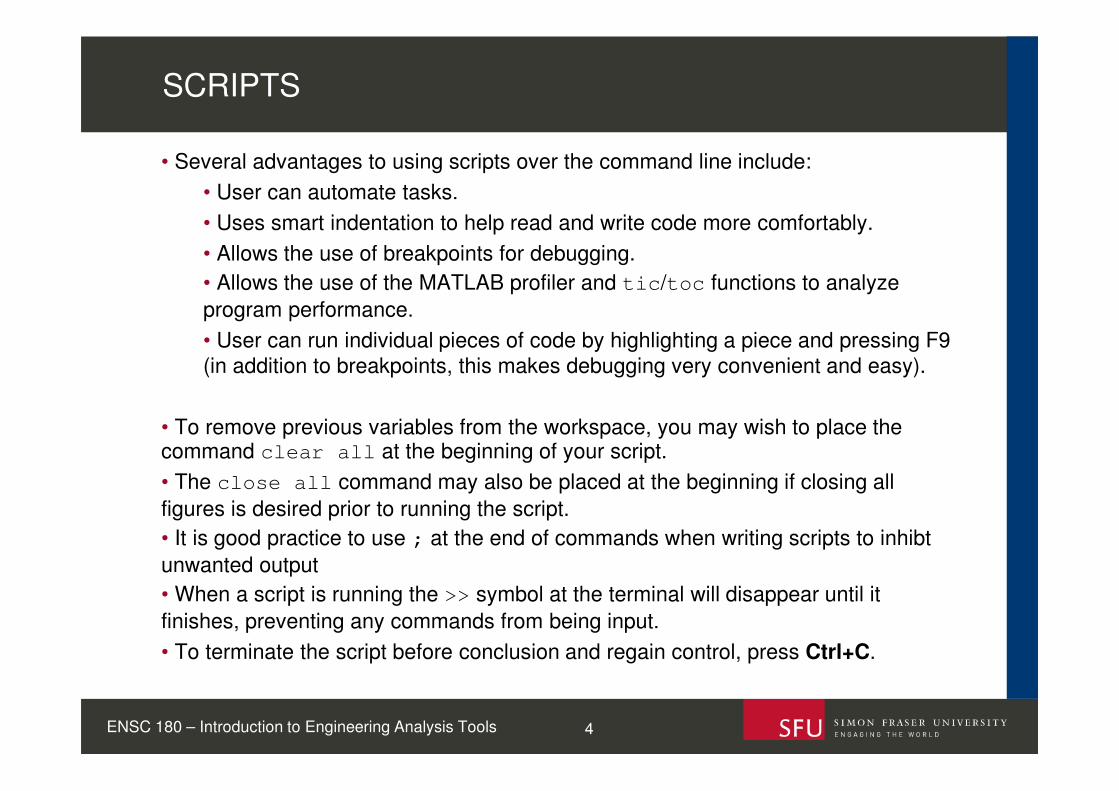
• Several advantages to using scripts over the command line include:

• User can automate tasks.

• Uses smart indentation to help read and write code more comfortably.

• Allows the use of breakpoints for debugging.

• Allows the use of the MATLAB profiler and tic/toc functions to analyze

program performance.

• User can run individual pieces of code by highlighting a piece and pressing F9

(in addition to breakpoints, this makes debugging very convenient and easy).

• To remove previous variables from the workspace, you may wish to place the command clear all at the beginning of your script.

• The close all command may also be placed at the beginning if closing all

figures is desired prior to running the script.

• It is good practice to use ; at the end of commands when writing scripts to inhibt

unwanted output

• When a script is running the >> symbol at the terminal will disappear until it

finishes, preventing any commands from being input.

• To terminate the script before conclusion and regain control, press Ctrl+C.

SCRIPTS


5

• Word wrap for comments is automatically enabled in scripts so that each line fits in

the viewable window to prevent the need for horizontal scrolling.

• Making use of ellipses ... can help make scripts more readable when there are

long statements of code:

A = [1 2 3 4 5 6; ...

6 5 4 3 2 1];

• This can also be used to make long character strings by concatenating two shorter

strings together:

mystring = ['Accelerating the pace of ' ...

'engineering and science'];

ELLIPSES


6

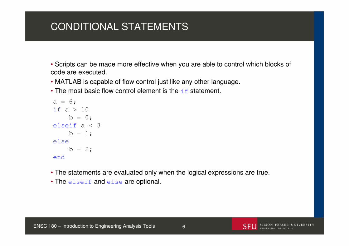
• Scripts can be made more effective when you are able to control which blocks of

code are executed.

• MATLAB is capable of flow control just like any other language.

• The most basic flow control element is the if statement.

• The statements are evaluated only when the logical expressions are true.

• The elseif and else are optional.

CONDITIONAL STATEMENTS

a = 6;

if a > 10

b = 0;

elseif a < 3

b = 1;

else

b = 2;

end


7

• A for loop uses a counter to repeatedly execute the block of code within it.

• It follows the syntax: for index=values, statements, end.

• The values portion of the syntax can take several forms, one of which is:

• In this case, the index ii is incremented by an optional step size until it reaches 8.

• A is initialized as an empty matrix and its size is constantly updated as we add to it

during each iteration of the loop.

• Note that the name of the index variable is ii rather than the traditional i,

commonly used in C/C++. Recall that i is reserved for the complex unit.

• Can create character indices as well, e.g. ii = 'a':'z'.

• The value of the index should never be modified by the statements inside the loop.

FOR LOOPS

A = [];

for ii = 2:2:8

A = [A ii]

end

ii = 2

ii = 4

ii = 6

ii = 8

A = 2

A = 2 4

A = 2 4 6

A = 2 4 6 8


8

• values can also be defined without the use of the colon operator:

A = zeros(1,3); %pre-allocate space

k = 1; %count loop iterations

valueMatrix = [1 2 3;

5 6 7];

for jj = valueMatrix

fprintf('iteration %d:\n', k)

A(k) = jj(1) + jj(2);

jj, A %display variables on terminal

k = k + 1;

end

• Here, the loop index is a column vector obtained fromsubsequent columns of the matrix valueMatrix on

each iteration.

• Even if column vector indices are not desired, this

method allows the use of irregular loop indices.

FOR LOOPS

iteration 1:

jj = 1

5

A = 6 0 0

iteration 2:

jj = 2

6

A = 6 8 0

iteration 3:

jj = 3

7

A = 6 8 10


9

• Note that in the previous example, we pre-allocated space to matrix A rather than

letting MATLAB resize it on every iteration. Use functions like length and size

along with the colon operator to determine loop indices after pre-allocating space.

A B

• Which of the two solutions will compute faster?

PRE-ALLOCATING SPACE TO VARIABLES

tic

for ii = 1:2000

for jj = 1:2000

A(ii,jj) = ii + jj;

end

end

toc

Elapsed time is 12.357 seconds

tic

A = zeros(2000, 2000);

for ii = 1:size(A,1)

for jj = 1:size(A,2)

A(ii,jj) = ii + jj;

end

end

toc



10

• Note that in the previous example, we pre-allocated space to matrix A rather than

letting MATLAB resize it on every iteration (computationally expensive).

• For very large loops, it is good practice to always pre-allocate space:

A B

• Use functions like length and size along with the colon operator to determine

loop indices after pre-allocating space.

PRE-ALLOCATING SPACE TO VARIABLES

tic

for ii = 1:2000

for jj = 1:2000

A(ii,jj) = ii + jj;

end

end

toc


tic

A = zeros(2000, 2000);

for ii = 1:size(A,1)

for jj = 1:size(A,2)

A(ii,jj) = ii + jj;

end

end

toc



11

• A while loop repeats for as long as the condition remains true.

• This can be very useful for things such as numerical approximation, where we

aren’t sure of the exact number of iterations.

• E.g.: we want to approximate π using Newton’s method and we want the estimate

to be within 10-32 of the actual value:

• We see that it takes 6 iterations to achieve our desired precision using an initial estimate of x = 2.

WHILE LOOPS

x = 2;

k = 0;

error = inf;

error_threshold = 1e-32;

while error > error_threshold

x = x - sin(x)/cos(x);

error = abs(x - pi);

k = k + 1;

end

>> x

x =

3.141592653589793

>> k

k =

6


12

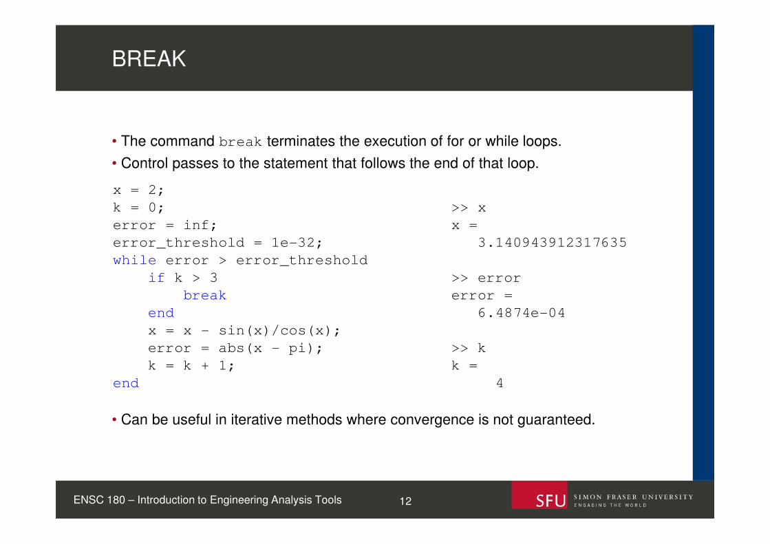
• The command break terminates the execution of for or while loops.

• Control passes to the statement that follows the end of that loop.

• Can be useful in iterative methods where convergence is not guaranteed.

BREAK

x = 2;

k = 0;

error = inf;

error_threshold = 1e-32;

while error > error_threshold

if k > 3

break

end

x = x - sin(x)/cos(x);

error = abs(x - pi);

k = k + 1;

end

>> x

x =

3.140943912317635

>> error

error =

6.4874e-04

>> k

k =

4


13

• In a switch statement, the input is matched against several different values and a

block of code is executed for the case where the match is correct:

x = 't';

switch x

case 2

disp('x is 2')

case -1

disp('x is -1')

case 't'

disp('x is the character t')

otherwise

disp('x is not 2, -1, or t')

end

x is the character t

SWITCH STATEMENTS


14

• Attempts to evaluate an expression; if an error occurs, the statement inside the

catch block is executed.

• After the error is “caught”, the script continues after the end of the try statement.

• In this example, b only has 3 elements so an error occurs when the script

attempts to access the 4th and 5th element.

• By using try/catch, MATLAB no longer terminates the script at this error.

TRY/CATCH STATEMENTS

a = 1:5;

b = 1:3;

for ii = 1:length(a)

try

c(ii) = a(ii) + b(ii)

catch

disp('b is too small')

end

end

c =

2

c =

2 4

c =

2 4 6

b is too small

b is too small


15

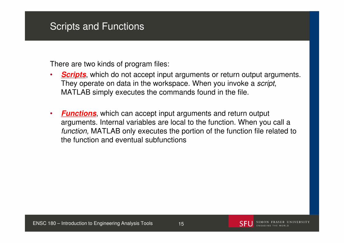
There are two kinds of program files:

• Scripts, which do not accept input arguments or return output arguments.

They operate on data in the workspace. When you invoke a script,

MATLAB simply executes the commands found in the file.

• Functions, which can accept input arguments and return output

arguments. Internal variables are local to the function. When you call a

function, MATLAB only executes the portion of the function file related to

the function and eventual subfunctions

Scripts and Functions


16

• Functions are useful for automating frequently used tasks and subroutines.

• For example, we can write a script to calculate the area of a triangle:

• To perform this calculation again for a different triangle, we would have to modify the values of b and h in the script and re-run it.

• Rather than doing this, we can simply convert this task into a function [1].

function a = triarea(b, h)

a = 0.5*(b.* h);

end

• The calculation can now be performed repeatedly without any modifications:

FUNCTIONS

b = 5;

h = 3;

a = 0.5*(b.* h)

a =

7.5000

a1 = triarea(1,5)

a2 = triarea(2,10)

a1 = 2.5000

a2 = 10


17

• Functions must be defined in an independent file, that must be saved in the work folder

• MATLAB files can contain code for more than one function.

• The first function in the file (the main function) is visible to functions in other files, or

you can call it from the command line.

• Additional functions within the file are called local functions. Local functions are only

visible to other functions in the same file. They are equivalent to subroutines in other

programming languages, and are sometimes called subfunctions.

• Local functions can occur in any order, as long as the main function appears first. Each

function begins with its own function definition line.

FUNCTION FILES


18

• Functions have their own independent workspaces and everything that occurs

inside is hidden from the main workspace.

• From the previous example, if my main workspace has a variable b already

defined, calling triarea will not interfere with this variable even though we use a

variable also called b inside of it.

• Finally, any lines after the function name which begin with % will serve as the help

text when the function is called using the help command.

FUNCTIONS


% This function calculates

% the area of a triangle.

% INPUTS: b - base, h - height

% OUTPUTS: a – area

a = 0.5*(b.* h);

end

>> help triarea

This function calculates

the area of a triangle.

INPUTS: b - base, h - height

OUTPUTS: a - area


>> b = 99;

>> a3 = triarea(2,4);

>> b

b =

99

19

Solution A: Running a simple Script

Solution B: Calling a Function


a = 0.5*(b.* h);

end

FUNCTIONS

b = 5;

h = 3;

a = 0.5*(b.* h)

a =

7.5000

a1 = triarea(5,3) a1 = 7.5000


Which of the two solutions is faster ?

20

Solution A: Running a simple Script

Solution B: Calling a Function


a = 0.5*(b.* h);

end

FUNCTIONS

b = 5;

h = 3;

a = 0.5*(b.* h)

a =

7.5000

a1 = triarea(5,3) a1 = 7.5000


The first solution is faster as it does not involve seeking the file system for the function and

calling it (control overhead). Functions are useful for code readability and efficiency, but do

not speed up computation; on the contrary, they involve a little overhead

Elapsed time is 0.000288 seconds.

Elapsed time is 0.0003390 seconds.

21

• Function handles provide a way to create anonymous functions, i.e., one line

expression functions that do not have to be defined in .m files.

• A function handle is a MATLAB data type and can therefore be passed into other

functions to be called indirectly.

>> f = @(x) exp(-2*x);

>> x = 0:0.1:2;

>> plot(x, f(x))

• We have assigned the function e-2x

to function handle f and evaluated

it at each point in vector x.

• To integrate e-2x from 0.2 to 0.8, wecan use f as an input argument to the

MATLAB function integral:

>> integral(f, 0.2, 0.8)

ans =

0.2342

FUNCTION HANDLES

0 0.5 1 1.5 20

0.2

0.4

0.6

0.8

1

x

f(x)


22

• In a matrix, each element contains a single value and all elements in the matrix must be of a single type, e.g. double, char, logical, etc.

• A cell array is a data structure with indexed containers (like the elements of a

matrix) called cells.

• Each cell, can store any type of data and can vary in size.

• Cell arrays can be created using the same syntax as a matrix, except curly brackets {} are used instead of square brackets [].

>> A = {[1 2; 3 4], 27; 'Alice', {1, 2, 3}}

A =

[2x2 double] [ 27]

'Alice' {1x3 cell}

• In this example, A is a 2-by-2 cell array containing different types of arrays with

different sizes.

CELL ARRAYS


23

•To retrieve the contents of a cell, use indexing with curly brackets.

>> A = {[1 2; 3 4], 27; 'Alice', {1, 2, 3}}

>> B = A{1,1}

B =

1 2

3 4

• To retrieve a cell itself, use indexing with round brackets.

>> C = A(1,:)

C =

[2x2 double] [27]

• Here, C is a 1-by-2 cell array.

CELL ARRAYS


24

• Like the cell array, a structure is another method of storing heterogeneous data.

• A structure is composed of data containers called field, which are accessed by

strings.

• For example, we want to store student assignment grades in a structure:

STRUCTURES

student.name = 'John Doe';

student.id = '[email protected]';

student.number = 301073268;

student.grade = [100, 75, 73; ...

95, 91, 85.5; ...

100, 98, 72];

student =

name: 'John Doe'

id: '[email protected]'

number: 301073268

grade: [3x3 double]


25

• Records for additional students can be added by including an index after the name

of the structure:

student(2).name = 'Ann Lane';

student(2).id = '[email protected]';

student(2).number = 301078853;

student(2).grade = [95, 95, 100; 100, 82, 85; 90, 97, 100];

STRUCTURES

student =

1x2 struct array

with fields:

name

id

number

grade


26

• Choosing between cell arrays and structures is mostly a matter of personal

preference and code clarity.

• The containers of a cell array are referred to by their index, whereas the containers

of a structure are referred to by their names.

student_data(1,:) = {'John Doe', '[email protected]', 301073268, ...

[100, 75, 73; 95, 91, 85.5; 100, 98, 72]};

student_data(2,:) = {'Ann Lane', '[email protected]', 301078853, ...

[95, 100, 90; 95, 82, 97; 100, 85, 100]};

student_data =

'John Doe' '[email protected]' [301073268] [3x3 double]

'Ann Lane' '[email protected]' [301078853] [3x3 double]

• Here, we accomplish what we did previously using a cell array.

• Rather than fetching the 2nd student’s no. by student(2).number, we would do

student_data{2,3}, since column 3 is where student numbers are stored.

• Since this is not as intuitive, we may conclude that a structure was a better choice.

CELL ARRAYS VS. STRUCTURES


27

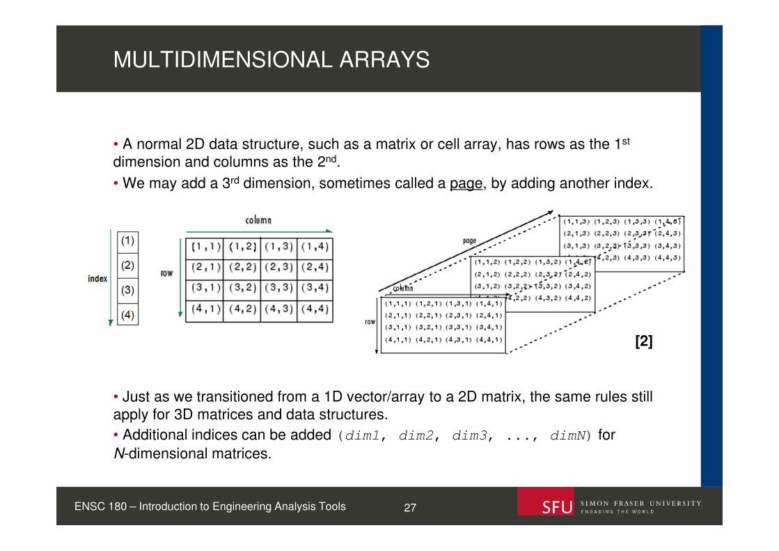
• A normal 2D data structure, such as a matrix or cell array, has rows as the 1st

dimension and columns as the 2nd.

• We may add a 3rd dimension, sometimes called a page, by adding another index.

• Just as we transitioned from a 1D vector/array to a 2D matrix, the same rules still

apply for 3D matrices and data structures.

• Additional indices can be added (dim1, dim2, dim3, ..., dimN) for

N-dimensional matrices.

MULTIDIMENSIONAL ARRAYS


[2]

28

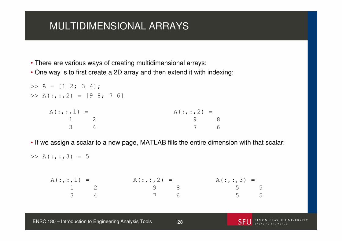
• There are various ways of creating multidimensional arrays:

• One way is to first create a 2D array and then extend it with indexing:

>> A = [1 2; 3 4];

>> A(:,:,2) = [9 8; 7 6]

• If we assign a scalar to a new page, MATLAB fills the entire dimension with that scalar:

>> A(:,:,3) = 5



A(:,:,1) =

1 2

3 4

A(:,:,2) =

9 8

7 6

A(:,:,1) =

1 2

3 4

A(:,:,2) =

9 8

7 6

A(:,:,3) =

5 5

5 5

29

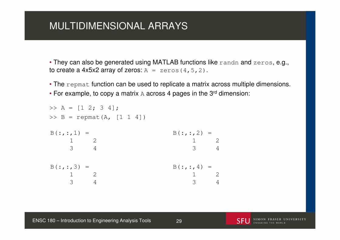
• They can also be generated using MATLAB functions like randn and zeros, e.g.,

to create a 4x5x2 array of zeros: A = zeros(4,5,2).

• The repmat function can be used to replicate a matrix across multiple dimensions.

• For example, to copy a matrix A across 4 pages in the 3rd dimension:

>> A = [1 2; 3 4];

>> B = repmat(A, [1 1 4])



B(:,:,1) =

1 2

3 4

B(:,:,2) =

1 2

3 4

B(:,:,3) =

1 2

3 4

B(:,:,4) =

1 2

3 4

30

• Examples of matrix concatenation on different dimensions:

• A = [ 1 2 ; 3 4 ] B = [ 5 6; 7 8]



• Sets of matrices can be concatenated along any dimension using the cat function C

= cat(dim, A, B)

31

• Sets of matrices can be concatenated along any dimension using the cat function

C = cat(dim, A, B)

>> A1 = [0 2; 4 6];

>> A2 = [1 3; 5 9];

>> B = cat(3, A1, A2)

>> C = cat(4, B, B)



B(:,:,1) =

0 2

4 6

B(:,:,2) =

1 3

5 9

C(:,:,1,1) =

0 2

4 6

C(:,:,2,1) =

1 3

5 9

C(:,:,1,2) =

0 2

4 6

C(:,:,2,2) =

1 3

5 9

C = cat(dim, A, B)C = cat(dim, A, B)

32

[1] MathWorks. (2013). “Scripts vs. Functions” [Online]. Available:

http://www.mathworks.com/help/matlab/matlab_prog/scripts-and-functions.html

[Accessed Sep. 30, 2013].

[2] MathWorks. (2013). “Multidimensional Arrays” [Online]. Available:

http://www.mathworks.com/help/matlab/math/multidimensional-arrays.html

[Accessed Sep. 30, 2013].

BIBLIOGRAPHY


1389642901 358 ensc180-02-scripts flow control and data structures

Documents

script file

matlab terminal

script command cd

series of matlab commands

matlab profiler

path matlab r2012b

command line

end of commands