14. magnitude and color systems
TRANSCRIPT

ASTR 511/O’Connell Lec 14 1
MAGNITUDE AND COLOR SYSTEMS
INTRODUCTION
“Magnitudes” are an ancient and arcane, but by now unchangeable, way ofcharacterizing the brightnesses of astronomical sources. They wereintroduced by the Greek astronomer Hipparchus ca. 130 BC. He arrangedthe visible stars in order of apparent (naked eye) brightness on a scale thatran from 1 to 6, with stars ranked “1” being the brightest. The ranks werecalled magnitudes. The faintest stars visible to the eye under excellent skyconditions were ranked as sixth magnitude.
Much later it became clear that because of the way the human eye respondsto a stimulus, magnitudes were proportional to the logarithm of the EMpower entering the eye from the source.
The modern magnitude system has been quantified as follows:
m = −2.5 log10f(i)
Q(i)
where f is the mean spectral flux density (see Lec. 2) from a source at thetop of the Earth’s atmosphere averaged over a defined band and Q is anormalizing constant for that band.
Although this definition looks peculiar, it offers two important practicalconveniences: (1) Cosmic sources have an enormous range of brightness,and the magnitude system provides a quick shorthand for expressing thesewithout referring to exponents. (2) The change of magnitude caused by agiven (small) fractional change in the flux density of a source is numericallyequal to the fractional change. E.g., a 5% error in flux density produces a0.05 mag change.

ASTR 511/O’Connell Lec 14 2
Nonetheless, magnitudes are the source of considerable confusion amongprofessional astronomers because there is not one magnitude system butinstead several. For historical reasons within subfields, the definitions differin two ways: (1) The spectral flux density can be expressed either as fν(ν)or fλ(λ). (2) The normalizing constant Q(i) differs among the systems; andeven within a given system, it can differ with waveband.
The most widely used magnitude system through the year 2000 was basedon a set of normalizing constants derived from the spectrum of the brightstar Vega. We are now slowly moving to “absolute” systems based oncalibrations in terms of physical flux units.
I. MONOCHROMATIC MAGNITUDE SYSTEMS
In Lecture 2 we introduced a “monochromatic” magnitude system, which isdefined as:
mλ(λ) ≡ −2.5 log10 Fλ(λ) − 21.1
where Fλ(λ) is the spectral flux density per unit wavelength of a source
at the top of the Earth’s atmosphere in units of erg s−1 cm−2 A−1
.This is also known as the “STMAG” system because it is standard forthe Hubble Space Telescope. For more details, see the Synphot User’sGuide at STScI.
The corresponding system based on flux per unit frequency is
mν(λ) ≡ −2.5 log10 Fν(λ) − 48.6
where Fν(λ) is in units of erg s−1 cm−2 Hz−1. This is also known asthe “AB” or “ABν” system. This system has been adopted by the SloanDigital Sky Survey and GALEX. (The resulting magnitudes are thereforevery different from the STMAG system in the UV, for example.)
These are the most intuitively obvious of the various magnitude scales usedby astronomers since the normalizing constants are the same at all

ASTR 511/O’Connell Lec 14 3
wavelengths, and magnitudes are easily convertible to physical flux unitsregardless of the wavelength observed.
The zero points are defined to coincide with the zero point of the widelyused “visual” or standard “broad-band” V magnitude system: i.e.
mλ(5500 A) = mν(5500 A) = V
However, the infinitesimal wavelength range inherent in the fλ or fν
definitions cannot actually be measured in practice. The monochromaticmagnitudes are estimates based on observations made in wider bands, andthe conversion to flux can only be as good as broader-band observations canbe calibrated. In fact, these systems are the stepchildren of more basicbroad-band systems in use by astronomers for over 100 years—but which aremore awkward in definition and usage.
II. FILTER PHOTOMETRY SYSTEMS
Broad-band magnitude systems were introduced into astronomy byphotography, which offered multi-wavelength response not confined to theacceptance band of the human eye (the “visual” band). As photoelectricdetectors were implemented, systems defined using filters of varying widthsproliferated. (Consult the bibliography for details.)
It is extremely difficult to calibrate astronomical photometric equipment theway one would calibrate laboratory equipment. Observations are made underfield conditions, and there are no easily deployable laboratory flux standards.Each piece of photometric equipment, wavelength isolator, and telescopehas different properties, and the throughput of the Earth’s atmospherechanges nightly.
Thus, astronomical magnitude systems are defined in terms of the brightnessof sources in specific wavebands relative to a set of “standard stars”selected by agreement. These relative brightnesses are better determinedthan any “absolute fluxes” which might derived from them. (Therefore,much astrophysical analysis is of the magnitudes rather than the fluxes.)
Apart from the difficulty of flux calibration, broad-band systems suffer fromthe fact that they are indeed broad, with typical optical bandwidths in the

ASTR 511/O’Connell Lec 14 4
range ∼500–2000 A. The reason for this is, of course, to enable study offaint astronomical sources. But wide bands introduce a host of difficultiesarising from the fact that cosmic SED’s and instrumental responses canchange significantly within the bands.
A brief history:
• The original visual system was, of course, based on the response of thehuman eye. In the 19th century, various clever designs emerged whichallowed simultaneous comparative “photometry” of the brightnesses oftwo stars or of a star and a calibration source. But visual measures werenever very precise.
• The photographic plate gave rise to the “photovisual” system (Pv),using filters which approximated the eye’s response, and the“photographic” system (Pg), which used a bluer filter to take advantageof the enhanced photographic response there. Aperture photometersand densitometers allowed quantitative extraction of information storedon a plate (subject, though, to significant uncertainties owing to thenonlinear and nonuniform responses of emulsions).
• The first photoelectric filter photometry system to be used for largenumbers of measures of stars and galaxies was the “6-color” system ofStebbins and Whitford (1935-1960).
• The 1P21 photomultiplier tube (1945), with dramatically improvedperformance in both sensitivity and noise rejection (especially ifoperated in pulse-counting mode), ushered in a new era in photoelectricphotometry. It had a CsSb (“S-4”) photocathode, with excellent blue(4000 A) sensitivity but a red cutoff at about 6300 A. A number of laterPMT designs (e.g. S-1, S-20) extended sensitivity to 8000-10000 A.
• The prototype broad-band system for those in wide use today was the“UBV” system of Johnson & Morgan (ApJ, 117, 486, 1953). This wascarefully defined in terms of specific choices of filter glass matched tothe 1P21 PMT and the energy distributions of stars (see plot below). Itwas normalized to the SED of Vega.
• The UBV system was so successful in applications to stellar evolution,stellar populations, interstellar dust, and extragalactic astronomy that itwas energetically extended to the red and infrared (R,I,J,H,K).Unfortunately, this work was undertaken by numerous workers usingdifferent filters and detectors, resulting in a confusing and incompatible

ASTR 511/O’Connell Lec 14 5
set of definitions (especially in R and I). Only in the last 20 years havethese systems been consolidated (see bibliographic entries for Bessell).
• The basic broad-band system in use today covers the optical range(3300-10000 A) with UBVRI, the near-infrared (1.0-2.4µ) with JHK,and part of the mid-infrared (3.0-10µ) with LMN. In the future, themost widely used bands in the LMN region will be the four defined bythe IRAC camera on the Spitzer Space Telescope.
• The Stromgren system was the first intermediate-band system to bewidely used. Its filters (180-300 A width) were tailored to measureabundance, temperature, and surface gravity effects in AF stars.Various other systems (e.g. DDO) extend this approach to later typestars and galaxies.
• Other useful broad-band systems include the Washington system(intended for faint GK stars) and the Thuan-Gunn system. The latter islike UBVRI but with filters optimized for faint galaxies by rejectingnight sky lines; it is used for the Sloan Digital Sky Survey.
• You can find transmission data for all the widely used filter systems at:http://voservices.net/filter/.

ASTR 511/O’Connell Lec 14 6
The Johnson-Morgan UBV filter system.
Approximate central wavelengths and bandwidths are:
Band < λ > (A) ∆λ (A)
U 3600 560B 4400 990V 5500 880

ASTR 511/O’Connell Lec 14 7
Standard UBVRI broad-band filter response curves (KPNO).
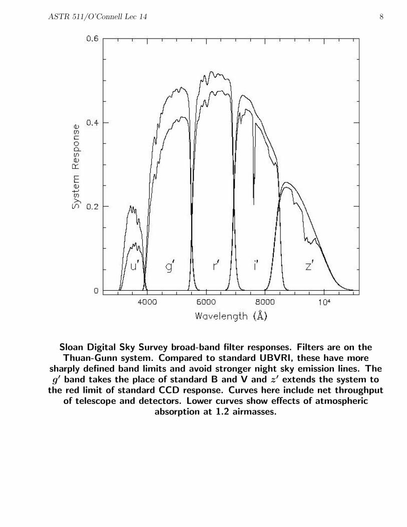
ASTR 511/O’Connell Lec 14 8
Sloan Digital Sky Survey broad-band filter responses. Filters are on theThuan-Gunn system. Compared to standard UBVRI, these have more
sharply defined band limits and avoid stronger night sky emission lines. Theg′ band takes the place of standard B and V and z′ extends the system to
the red limit of standard CCD response. Curves here include net throughputof telescope and detectors. Lower curves show effects of atmospheric
absorption at 1.2 airmasses.

ASTR 511/O’Connell Lec 14 9
III. THE VEGA MAGNITUDE SYSTEM
Following Johnson & Morgan, the set of calibrator stars for most filterphotometry systems is defined by one “primary standard,” the bright starVega (α Lyrae), which in turn has been coupled through an elaboratebootstrap technique to a large set of “secondary” standards. The bootstrapinvolved extensive observational filter photometry and spectrophotometry aswell as theoretical modeling of stellar atmospheres.
Ideally, the Vega magnitude system (or “vegamag”) is defined as follows:
o Let Ri(λ) be a transmission function for a given band i. R is usuallydetermined primarily by a filter.
o Then for a source whose spectral flux density at the top of the Earth’satmosphere is Fλ(λ), the broad-band magnitude mi is
mi = −2.5 log10
∫Ri(λ)λFλ(λ)dλ∫
Ri(λ)λF VEGAλ (λ)dλ
+ 0.03
where 0.03 is the V magnitude of Vega. The system is based onspectral flux density per unit wavelength.
o Here we have assumed a photon-counting detector, so that the systemresponse is proportional to the photon rate. This is the origin of theadditional λ term in the expression above (the photon rate is [λ/hc]Fλ).
o Vega was chosen as the primary standard because it is easily observablein the northern hemisphere for more than 6 months of the year andbecause it has a relatively smooth spectral energy distribution comparedto later type stars. Bright stars with the same spectral type arerelatively common.
o The SED of Vega is shown on the next page, and an IDL save filecontaining a digital version (theoretical) of the SED is linked to theLectures web page.
o Vital statistics for Vega (from Kurucz): Spectral type A0 V. Effectivetemperature Te = 9550 K. Surface gravity log g = 3.95. Metalabundance log Z/Z� = −0.5.

ASTR 511/O’Connell Lec 14 10
Plot of zeropoint spectra in three different magnitude systems.(Note: ordinate is photon flux, not energy flux.)
Although Vega has a reasonably smooth energy distribution, as compared,for example, to an M star, there are obviously large changes in the vegamag
normalizing constants with wavelength.

ASTR 511/O’Connell Lec 14 11
Implications of this definition:
o In each band, the system weights the photon SED of a source by thedefined response function Ri(λ). This is usually not a “top-hat”function with a flat top and vertical sides.
The Ri’s for the basic bands are described. for example, in thearticles by Bessell in the bibliography.
Even under the best circumstances, any particular equipment willdiffer slightly in Ri from the standard system. This means thattransformations to the standard system must be part of anyphotometric reduction.
Calibration is more difficult the broader is the band. This is becauseof changes in the source SED and the weighting function within theband. Cf. equation (2) of Lecture 12.
o For Vega, or any other A0 V type star,
mi = mj = V for all i, j
o The zero point of the system is defined by the SED of an A0 V star,which means that the zero point differs from band to band.
Even if mi = mj, the corresponding mean fluxes, < Fλ >i and< Fλ >j are generally not equal. From the plot of Vega’s SED, onecan see that the flux zero point at 1µ, for instance, is significantlylower than at 5500 A.
This is a major departure from the monochromatic systems, forwhich equal magnitudes imply equal flux densities.
o With modern highly sensitive detectors, Vega is too bright to observedirectly for calibration. Instead, one must observe (every night) aselection of secondary or tertiary standards.
o The actual zero points of the system are defined by the full set ofsecondary standard stars. Small residual “closure” errors mean that themeasured values in practice will depend on the particular set ofstandards observed on a given night.

ASTR 511/O’Connell Lec 14 12
IV. FLUX CALIBRATION OF THE VEGA SYSTEM
The zero point of the Vega system is based on high quality data fromPMT-based spectrophotometers obtained by Oke, Schild, Hayes, andLatham ca. 1967-1975 (see bibliography). These spectra were calibrated bydirect observations of nearby laboratory light sources (e.g. platinumfurnaces), though this introduced many complications (e.g. horizontalextinction across the mountain tops).
These data sets have been melded with increasingly high fidelity syntheticstellar spectra (theoretical) to extend and consolidate the system across thevarious bands. The best current calibration for the UBVRIJHK system is byBessell, Castelli, & Plez (1998, see bibliography and next page). You werealready introduced to the zero point of the V-band system in Lecture 2:
Fluxes for a V = 0 star of spectral type A0 V at 5450A:
f0λ = 3.63 × 10⁻⁹ erg s−1 cm−2 A
−1, or
f0ν = 3.63 × 10⁻²⁰ erg s−1 cm−2 Hz−1, or
φ0λ = f0
λ/hν = 1005 photons cm−2 s−1 A−1
Note that the effective wavelength of the filter shifts with the SED of thesource and is closer to 5500 A for G-K stars.
The flux zero point in filters other than V is then defined by the spectralenergy distribution of an A0 V star. The relationship between themagnitude in a given filter and the mean flux in that filter is then given by:
mi = −2.5 log10
(< Fλ >i
F0,i
)
where F0,i is the zero point for band i as given in the Bessell listing
(units: erg s−1 cm−2 A−1
).

ASTR 511/O’Connell Lec 14 13
BROAD BAND SYSTEM ZEROPOINTS (BESSELL ET AL. 1998)
Bessell’s 1998 values for the effective wavelength of each filter (for an A0 Vspectral type) and the corresponding flux zeropoints are given above. These,together with mean colors for various spectral types on the Johnson system(which differs from Bessell), will also be handed out.
Note two important typos in the published table: the fourth row of the tableshould be labeled zp(fν) and the fifth row should be labeled zp(fλ).

ASTR 511/O’Connell Lec 14 14
V. COLORS
A “color” is simply a difference between magnitudes for a given source intwo different bands:
Cij ≡ mi − mj = −2.5 log10
(< Fλ >i
< Fλ >j
)+ constij
where the constant is a function of the zeropoints of the two bands.
Colors measure the slope of the spectral energy distribution between bands iand j.
Note that the definition is such that a more positive color implies a largerflux in the second (j) band.
It is usual, though not universal, that the two bands are entered in order ofincreasing wavelength.
Colors are used in all of the magnitude systems defined above. However, thehistorical precedent of the classic Johnson-Morgan system is such that labelssuch as UBVRIJK are understood to refer to the Vega system unlessotherwise explicitly stated.
The V band is often a convenient reference, so colors like B-V, V-I, V-K arewidely used. The standard “UBV” system employs U-B and B-V. Coolsources which emit little light below 8000 A are often characterized by I-K,J-K, H-K, etc.

ASTR 511/O’Connell Lec 14 15
VI. ATMOSPHERIC EXTINCTION
The effect of atmospheric extinction on photometry (cf. Lec 4) is usuallyexpressed as:
mobs = mtrue + k(λ) sec Z
Here, mtrue is the magnitude of the source outside the Earth’s atmosphere,and mobs is the magnitude observed.
The “air mass,” sec Z, where Z is the angular zenith distance, is givenby the following expression (for plane-parallel geometry):
sec Z = [sin φ sin δ + cos φ cos δ cos h]−1
where φ is the latitude of the observatory, h is the hour angle of thesource, and δ is the declination of the source.
sec Z is the total atmospheric pathlength toward the source in units ofthe vertical pathlength. For best photometry, keep sec Z . 2.
k(λ) is the “extinction coefficient.”
Several different physical effects contribute to continuous extinction. Theseinclude Rayleigh scattering (∼ λ−4), ozone or H2O molecular absorption,and aerosol scattering. Each of these is characterized by a different effectivescale height, so that their mixture will change with altitude.
Extinction coefficients have been carefully measured for a number ofobservatories. A table for Palomar (Hayes & Latham 1975) is included onthe next page.
Ignoring its multi-component nature, approximate values of extinction for agiven site can be obtained from those for another (assuming a hydrostatic,isothermal atmosphere) as follows:
k(X1) = k(X0)exp
(−
[(X1 − X0)
H0
])where X1 and X0 are the altitudes of the two observatories and H0 is thescale height of the atmosphere (7950 meters for STP).

ASTR 511/O’Connell Lec 14 16
ASTR 511/O’Connell Lec 14 17
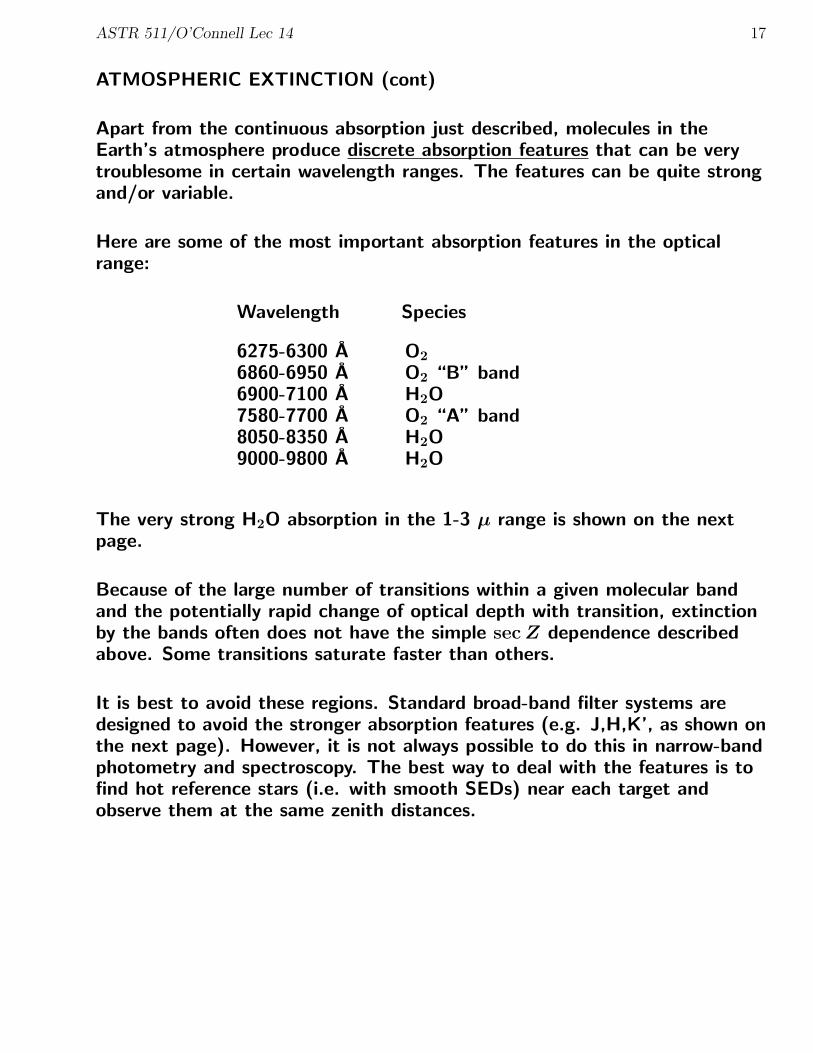
ATMOSPHERIC EXTINCTION (cont)
Apart from the continuous absorption just described, molecules in theEarth’s atmosphere produce discrete absorption features that can be verytroublesome in certain wavelength ranges. The features can be quite strongand/or variable.
Here are some of the most important absorption features in the opticalrange:
Wavelength Species
6275-6300 A O26860-6950 A O2 “B” band6900-7100 A H2O7580-7700 A O2 “A” band8050-8350 A H2O9000-9800 A H2O
The very strong H2O absorption in the 1-3 µ range is shown on the nextpage.
Because of the large number of transitions within a given molecular bandand the potentially rapid change of optical depth with transition, extinctionby the bands often does not have the simple sec Z dependence describedabove. Some transitions saturate faster than others.
It is best to avoid these regions. Standard broad-band filter systems aredesigned to avoid the stronger absorption features (e.g. J,H,K’, as shown onthe next page). However, it is not always possible to do this in narrow-bandphotometry and spectroscopy. The best way to deal with the features is tofind hot reference stars (i.e. with smooth SEDs) near each target andobserve them at the same zenith distances.

ASTR 511/O’Connell Lec 14 18
LINE ABSORPTION IN THE NEAR-IR
Transmission of the Earth’s atmosphere in the near-infrared. Absorption isdominated by H2O. Horizontal lines show the definitions of the J, H, and K’
photometric bands, which lie in relatively clean regions.

ASTR 511/O’Connell Lec 14 19
VII. PHOTOMETRIC CALIBRATION & REDUCTION
Calibration of photometric observations and reduction to the standardbroad-band system require observation of standard stars. These are used todetermine the effects of atmospheric extinction and the “transformation”between the response of your equipment and that of the standard system.
(i) Atmospheric transmission varies from night to night. You must makesufficient standard observations each night to calibrate thatindependently of other nights of your run.
(ii) However, you can use combined data from several nights to determinethe photometric transformations between your filter set and thestandard set.
(iii) Calibration can have strong color-dependent terms. This means thatyour standards must span the color range of your “unknowns.” Thelarger is that range, the larger is the standard set you need to observe.
(iv) Standards must be in the range of brightness appropriate for yourequipment.
Recalling equation (2) of Lecture 12, the count rate s (detected photonsper second in filter i) for a given source is
si ∝π
4D2
e
∫e−k(λ) sec Z Ti(λ)
Fλ(λ)
hνdλ
A. Narrow-Band Observations
If the bandwidth of the filter is so narrow that all of the terms in theabove expression are well approximated by mean values, then it isstraightforward to calibrate your data. The basic relation is:
mij = −2.5 log10 sijk − Ki sec Zk − ai
Here mij is the broad-band magnitude in filter i for standard star j;sijk is the count rate for the kth observation of this star at zenithdistance Zk.

ASTR 511/O’Connell Lec 14 20
Ki is the atmospheric extinction coefficient for band i and ai is thetransformation term between the local and standard photometricsystems.
The problem is to determine Ki and ai. More than two standard starobservations overdetermine the problem, but a large set of calibrationobservations gives valuable information on the scatter from random andsystematic errors (e.g. secular variation in atmospheric transparency).
B. Broad-Band Observations
The complexity here arises from the fact that the various terms in theproportion above are not constant across a broad-band filter. The effectof this will depend on the distribution of light of the source within theband, i.e. on the spectral slope of the source. This means there will becolor terms in both the effective atmospheric extinction and in thetransformation.
The normal approach to this problem is to first define “instrumentalcolors,” based on the relative count rates of two adjacent filters. Forexample:
Ci ≡ −2.5 log10
(si+1
si
)Then, rewrite the calibration equation above to include color terms inboth the extinction and transformation as follows:
mij = −2.5 log10 sijk − [K0,i + K1,iCi] sec Zk − a0,i − a1,iCi
The problem now includes 4 unknowns, and solution depends on havinga large range of color in the standard star observations. Many morestandard observations are needed than in the narrow-band case.
To provide a more robust solution, one normally starts with an estimateof the K terms (based on average atmospheric conditions) and iterateson those.
For more details on extinction corrections and reduction, see thebibliography (the Young articles are very thorough).