14.452 economic growthdaron acemoglu (mit) economic growth lecture 5 november 4, 2008 2 / 71...
TRANSCRIPT

14.452 Economic GrowthFall 2008
MIT OpenCourseWarehttp://ocw.mit.edu
For information about citing these materials or our Terms of Use, visit: http://ocw.mit.edu/terms.

14.452 Economic Growth: Lecture 5, NeoclassicalGrowth
Daron Acemoglu
MIT
November 4, 2008
Daron Acemoglu (MIT) Economic Growth Lecture 5 November 4, 2008 1 / 71

Introduction Introduction
Introduction
Ramsey or Cass-Koopmans model: di¤ers from the Solow model onlybecause it explicitly models the consumer side and endogenizessavings.
Beyond its use as a basic growth model, also a workhorse for manyareas of macroeconomics.
Daron Acemoglu (MIT) Economic Growth Lecture 5 November 4, 2008 2 / 71

Introduction Environment
Preferences, Technology and Demographics I
In�nite-horizon, continuous time.Representative household with instantaneous utility function
u (c (t)) , (1)
Assumption u (c) is strictly increasing, concave, twice continuouslydi¤erentiable with derivatives u0 and u00, and satis�es thefollowing Inada type assumptions:
limc!0
u0 (c) = ∞ and limc!∞
u0 (c) = 0.
Suppose representative household represents set of identicalhouseholds (normalized to 1).Each household has an instantaneous utility function given by (1).L (0) = 1 and
L (t) = exp (nt) . (2)
Daron Acemoglu (MIT) Economic Growth Lecture 5 November 4, 2008 3 / 71

Introduction Environment
Preferences, Technology and Demographics II
All members of the household supply their labor inelastically.Objective function of each household at t = 0:
U (0) �Z ∞
0exp (� (ρ� n) t) u (c (t)) dt, (3)
wherec (t)=consumption per capita at t,ρ=subjective discount rate, and e¤ective discount rate is ρ� n.
Objective function (3) embeds:Household is fully altruistic towards all of its future members, andmakes allocations of consumption (among household members)cooperatively.Strict concavity of u (�)
Thus each household member will have an equal consumption
c (t) � C (t)L (t)
Daron Acemoglu (MIT) Economic Growth Lecture 5 November 4, 2008 4 / 71
Introduction Environment
Preferences, Technology and Demographics III
Utility of u (c (t)) per household member at time t, total ofL (t) u (c (t)) = exp (nt) u (c (t)).
With discount at rate of exp (�ρt), obtain (3).
Assumption 40.ρ > n.
Ensures that in the model without growth, discounted utility is �nite.Will strengthen it in model with growth.
Start model without any technological progress.
Factor and product markets are competitive.
Production possibilities set of the economy is represented by
Y (t) = F [K (t) , L (t)] ,
Standard constant returns to scale and Inada assumptions still hold.
Daron Acemoglu (MIT) Economic Growth Lecture 5 November 4, 2008 5 / 71
Introduction Environment
Preferences, Technology and Demographics IV
Per capita production function f (�)
y (t) � Y (t)L (t)
= F�K (t)L (t)
, 1�
� f (k (t)) ,
where, as before,
k (t) � K (t)L (t)
. (4)
Competitive factor markets then imply:
R (t) = FK [K (t), L(t)] = f0 (k(t)). (5)
andw (t) = FL[K (t), L(t)] = f (k (t))� k (t) f 0 (k(t)). (6)
Daron Acemoglu (MIT) Economic Growth Lecture 5 November 4, 2008 6 / 71

Introduction Environment
Preferences, Technology and Demographics V
Denote asset holdings of the representative household at time t byA (t). Then,
A (t) = r (t)A (t) + w (t) L (t)� c (t) L (t)
r (t) is the risk-free market �ow rate of return on assets, andw (t) L (t) is the �ow of labor income earnings of the household.De�ning per capita assets as
a (t) � A (t)L (t)
,
we obtain:
a (t) = (r (t)� n) a (t) + w (t)� c (t) . (7)
Household assets can consist of capital stock, K (t), which they rentto �rms and government bonds, B (t).
Daron Acemoglu (MIT) Economic Growth Lecture 5 November 4, 2008 7 / 71

Introduction Environment
Preferences, Technology and Demographics VI
With uncertainty, households would have a portfolio choice betweenK (t) and riskless bonds.
With incomplete markets, bonds allow households to smoothidiosyncratic shocks. But for now no need.
Thus, market clearing )
a (t) = k (t) .
No uncertainty depreciation rate of δ implies
r (t) = R (t)� δ. (8)
Daron Acemoglu (MIT) Economic Growth Lecture 5 November 4, 2008 8 / 71
Introduction Environment
The Budget Constraint I
The di¤erential equation
a (t) = (r (t)� n) a (t) + w (t)� c (t)
is a �ow constraint
Not su¢ cient as a proper budget constraint unless we impose a lowerbound on assets.
Three options:1 Lower bound on assets such as a (t) � 0 for all t2 Natural debt limit (see notes).3 No-Ponzi Game Condition.
The �rst two are not always applicable, so the third is most general.
Daron Acemoglu (MIT) Economic Growth Lecture 5 November 4, 2008 9 / 71

Introduction Environment
The Budget Constraint II
Write the single budget constraint of the form:Z T
0c (t) L(t) exp
�Z T
tr (s) ds
�dt +A (T ) (9)
=Z T
0w (t) L (t) exp
�Z T
tr (s) ds
�dt +A (0) exp
�Z T
0r (s) ds
�Di¤erentiating this expression with respect to T and dividing L(t)gives (7).
Now imagine that (9) applies to a �nite-horizon economy ending atdate T .
Flow budget constraint (7) by itself does not guarantee thatA (T ) � 0.Thus in �nite-horizon we would simply impose (9) as a boundarycondition.
Daron Acemoglu (MIT) Economic Growth Lecture 5 November 4, 2008 10 / 71
Introduction Environment
The Budget Constraint III
In�nite-horizon case: no-Ponzi-game condition,
limt!∞
a (t) exp��Z t
0(r (s)� n) ds
�� 0. (10)
Transversality condition ensures individual would never want to havepositive wealth asymptotically, so no-Ponzi-game condition can bestrengthened to (though not necessary in general):
limt!∞
a (t) exp��Z t
0(r (s)� n) ds
�= 0. (11)
Daron Acemoglu (MIT) Economic Growth Lecture 5 November 4, 2008 11 / 71

Introduction Environment
The Budget Constraint IV
To understand no-Ponzi-game condition, multiply both sides of (9) by
exp��R T0 r (s) ds
�:
exp��Z t
0r (s) ds
� �Z T
0c (t) L(t)dt +A (T )
�=
Z T
0w (t) L (t) exp
��Z t
0r (s) ds
�dt +A (0) ,
Divide everything by L (0) and note that L(t) grows at the rate n,Z T
0c (t) exp
��Z t
0(r (s)� n) ds
�dt
+ exp��Z T
0(r (s)� n) ds
�a (T )
=Z T
0w (t) exp
��Z t
0(r (s)� n) ds
�dt + a (0) .
Daron Acemoglu (MIT) Economic Growth Lecture 5 November 4, 2008 12 / 71

Introduction Environment
The Budget Constraint V
Take the limit as T ! ∞ and use the no-Ponzi-game condition (11)to obtain Z ∞
0c (t) exp
��Z t
0(r (s)� n) ds
�dt
= a (0) +Z ∞
0w (t) exp
��Z t
0(r (s)� n) ds
�dt,
Thus no-Ponzi-game condition (11) essentially ensures that theindividual�s lifetime budget constraint holds in in�nite horizon.
Daron Acemoglu (MIT) Economic Growth Lecture 5 November 4, 2008 13 / 71

Characterization of Equilibrium De�nition of Equilibrium
De�nition of Equilibrium
De�nition A competitive equilibrium of the Ramsey economy consistsof paths [C (t) ,K (t) ,w (t) ,R (t)]∞t=0, such that therepresentative household maximizes its utility given initialcapital stock K (0) and the time path of prices[w (t) ,R (t)]∞t=0, and all markets clear.
Notice refers to the entire path of quantities and prices, not juststeady-state equilibrium.
De�nition A competitive equilibrium of the Ramsey economy consistsof paths [c (t) , k (t) ,w (t) ,R (t)]∞t=0, such that therepresentative household maximizes (3) subject to (7) and(10) given initial capital-labor ratio k (0), factor prices[w (t) ,R (t)]∞t=0 as in (5) and (6), and the rate of return onassets r (t) given by (8).
Daron Acemoglu (MIT) Economic Growth Lecture 5 November 4, 2008 14 / 71
Characterization of Equilibrium Household Maximization
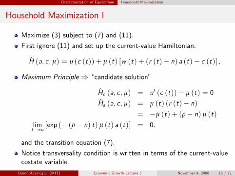
Household Maximization I
Maximize (3) subject to (7) and (11).
First ignore (11) and set up the current-value Hamiltonian:
H (a, c , µ) = u (c (t)) + µ (t) [w (t) + (r (t)� n) a (t)� c (t)] ,
Maximum Principle ) �candidate solution�
Hc (a, c , µ) = u0 (c (t))� µ (t) = 0
Ha (a, c , µ) = µ (t) (r (t)� n)= �µ (t) + (ρ� n) µ (t)
limt!∞
[exp (� (ρ� n) t) µ (t) a (t)] = 0.
and the transition equation (7).
Notice transversality condition is written in terms of the current-valuecostate variable.
Daron Acemoglu (MIT) Economic Growth Lecture 5 November 4, 2008 15 / 71

Characterization of Equilibrium Household Maximization
Household Maximization II
For any µ (t) > 0, H (a, c , µ) is a concave function of (a, c) andstrictly concave in c .
The �rst necessary condition implies µ (t) > 0 for all t.
Therefore, Su¢ cient Conditions imply that the candidate solution isan optimum (is it unique?)
Rearrange the second condition:
µ (t)µ (t)
= � (r (t)� ρ) , (12)
First necessary condition implies,
u0 (c (t)) = µ (t) . (13)
Daron Acemoglu (MIT) Economic Growth Lecture 5 November 4, 2008 16 / 71
Characterization of Equilibrium Household Maximization
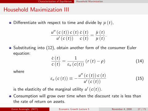
Household Maximization III
Di¤erentiate with respect to time and divide by µ (t),
u00 (c (t)) c (t)u0 (c (t))
c (t)c (t)
=µ (t)µ (t)
.
Substituting into (12), obtain another form of the consumer Eulerequation:
c (t)c (t)
=1
εu (c(t))(r (t)� ρ) (14)
where
εu (c (t)) � �u00 (c (t)) c (t)u0 (c (t))
(15)
is the elasticity of the marginal utility u0 (c(t)).
Consumption will grow over time when the discount rate is less thanthe rate of return on assets.
Daron Acemoglu (MIT) Economic Growth Lecture 5 November 4, 2008 17 / 71

Characterization of Equilibrium Household Maximization
Household Maximization IV
Speed at which consumption will grow is related to the elasticity ofmarginal utility of consumption, εu (c (t)).
Even more importantly, εu (c (t)) is the inverse of the intertemporalelasticity of substitution:
regulates willingness to substitute consumption (or any other attributethat yields utility) over time.Elasticity between dates t and s > t is de�ned as
σu (t, s) = �d log (c (s) /c (t))
d log (u0 (c (s)) /u0 (c (t))).
As s # t,
σu (t, s)! σu (t) = �u0 (c (t))
u00 (c (t)) c (t)=
1εu (c (t))
. (16)
Daron Acemoglu (MIT) Economic Growth Lecture 5 November 4, 2008 18 / 71

Characterization of Equilibrium Household Maximization
Household Maximization V
Integrating (12),
µ (t) = µ (0) exp��Z t
0(r (s)� ρ) ds
�= u0 (c (0)) exp
��Z t
0(r (s)� ρ) ds
�,
Substituting into the transversality condition,
0 = limt!∞
�exp (� (ρ� n) t) a (t) u0 (c (0)) exp
��Z t
0(r (s)� ρ) ds
��0 = lim
t!∞
�a (t) exp
��Z t
0(r (s)� n) ds
��.
Thus the �strong version�of the no-Ponzi condition, (11) has to hold.
Daron Acemoglu (MIT) Economic Growth Lecture 5 November 4, 2008 19 / 71

Characterization of Equilibrium Household Maximization
Household Maximization VI
Since a (t) = k (t), transversality condition is also equivalent to
limt!∞
�exp
��Z t
0(r (s)� n) ds
�k (t)
�= 0
Notice term exp��R t0 r (s) ds
�is a present-value factor: converts a
unit of income at t to a unit of income at 0.
When r (s) = r , factor would be exp (�rt). More generally, de�ne anaverage interest rate between dates 0 and t
r (t) =1t
Z t
0r (s) ds. (17)
Thus conversion factor between dates 0 and t is
exp (�r (t) t) ,
Daron Acemoglu (MIT) Economic Growth Lecture 5 November 4, 2008 20 / 71

Characterization of Equilibrium Household Maximization
Household Maximization VII
And the transversality condition
limt!∞
[exp (� (r (t)� n) t) a (t)] = 0. (18)
Recal solution to the di¤erential equation
y (t) = b (t) y (t)
is
y (t) = y (0) exp�Z t
0b (s) ds
�,
Integrate (14):
c (t) = c (0) exp�Z t
0
r (s)� ρ
εu (c (s))ds�
Once we determine c (0), path of consumption can be exactly solvedout.
Daron Acemoglu (MIT) Economic Growth Lecture 5 November 4, 2008 21 / 71
Characterization of Equilibrium Household Maximization
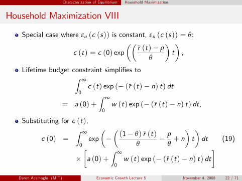
Household Maximization VIII
Special case where εu (c (s)) is constant, εu (c (s)) = θ:
c (t) = c (0) exp��
r (t)� ρ
θ
�t�,
Lifetime budget constraint simpli�es toZ ∞
0c (t) exp (� (r (t)� n) t) dt
= a (0) +Z ∞
0w (t) exp (� (r (t)� n) t) dt,
Substituting for c (t),
c (0) =Z ∞
0exp
���(1� θ) r (t)
θ� ρ
θ+ n�t�dt (19)
��a (0) +
Z ∞
0w (t) exp (� (r (t)� n) t) dt
�Daron Acemoglu (MIT) Economic Growth Lecture 5 November 4, 2008 22 / 71
Characterization of Equilibrium Equilibrium Prices
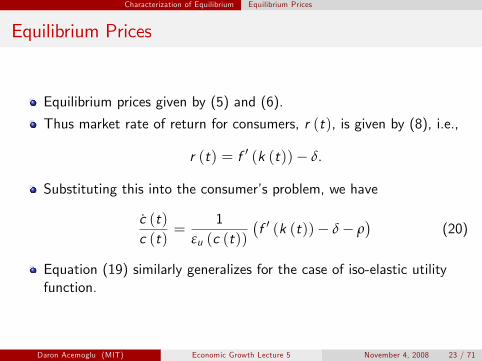
Equilibrium Prices
Equilibrium prices given by (5) and (6).
Thus market rate of return for consumers, r (t), is given by (8), i.e.,
r (t) = f 0 (k (t))� δ.
Substituting this into the consumer�s problem, we have
c (t)c (t)
=1
εu (c (t))
�f 0 (k (t))� δ� ρ
�(20)
Equation (19) similarly generalizes for the case of iso-elastic utilityfunction.
Daron Acemoglu (MIT) Economic Growth Lecture 5 November 4, 2008 23 / 71

Optimal Growth Optimal Growth
Optimal Growth I
In an economy that admits a representative household, optimalgrowth involves maximization of utility of representative householdsubject to technology and feasibility constraints:
max[k (t),c (t)]∞t=0
Z ∞
0exp (� (ρ� n) t) u (c (t)) dt,
subject tok (t) = f (k (t))� (n+ δ)k (t)� c (t) ,
and k (0) > 0.
Versions of the First and Second Welfare Theorems for economieswith a continuum of commodities: solution to this problem should bethe same as the equilibrium growth problem.
But straightforward to show the equivalence of the two problems.
Daron Acemoglu (MIT) Economic Growth Lecture 5 November 4, 2008 24 / 71

Optimal Growth Optimal Growth
Optimal Growth II
Again set up the current-value Hamiltonian:
H (k, c , µ) = u (c (t)) + µ (t) [f (k (t))� (n+ δ)k (t)� c (t)] ,
Candidate solution from the Maximum Principle:
Hc (k, c , µ) = 0 = u0 (c (t))� µ (t) ,
Hk (k, c , µ) = �µ (t) + (ρ� n) µ (t)
= µ (t)�f 0 (k (t))� δ� n
�,
limt!∞
[exp (� (ρ� n) t) µ (t) k (t)] = 0.
Su¢ ciency Theorem ) unique solution (H and thus the maximizedHamiltonian strictly concave in k).
Daron Acemoglu (MIT) Economic Growth Lecture 5 November 4, 2008 25 / 71
Optimal Growth Optimal Growth
Optimal Growth III
Repeating the same steps as before, these imply
c (t)c (t)
=1
εu (c (t))
�f 0 (k (t))� δ� ρ
�,
which is identical to (20), and the transversality condition
limt!∞
�k (t) exp
��Z t
0
�f 0 (k (s))� δ� n
�ds��
= 0,
which is, in turn, identical to (11).Thus the competitive equilibrium is a Pareto optimum and that thePareto allocation can be decentralized as a competitive equilibrium.
Proposition In the neoclassical growth model described above, withstandard assumptions on the production function(assumptions 1-40), the equilibrium is Pareto optimal andcoincides with the optimal growth path maximizing theutility of the representative household.
Daron Acemoglu (MIT) Economic Growth Lecture 5 November 4, 2008 26 / 71

Steady-State Equilibrium Steady State
Steady-State Equilibrium I
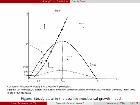
Steady-state equilibrium is de�ned as an equilibrium path in whichcapital-labor ratio, consumption and output are constant, thus:
c (t) = 0.
From (20), as long as f (k�) > 0, irrespective of the exact utilityfunction, we must have a capital-labor ratio k� such that
f 0 (k�) = ρ+ δ, (21)
Pins down the steady-state capital-labor ratio only as a function ofthe production function, the discount rate and the depreciation rate.
Modi�ed golden rule: level of the capital stock that does notmaximize steady-state consumption, because earlier consumption ispreferred to later consumption.
Daron Acemoglu (MIT) Economic Growth Lecture 5 November 4, 2008 27 / 71
Steady-State Equilibrium Steady State
c(t)
kgold0k(t)
k(0)
c’(0)
c’’(0)
c(t)=0
k(t)=0
k*
c(0)
c*
k
Figure: Steady state in the baseline neoclassical growth modelDaron Acemoglu (MIT) Economic Growth Lecture 5 November 4, 2008 28 / 71
Courtesy of Princeton University Press. Used with permission. Figure 8.1 in Acemoglu, K. Daron. Introduction to Modern Economic Growth. Princeton, NJ: Princeton University Press, 2009.
ISBN: 9780691132921.
Steady-State Equilibrium Steady State
Steady-State Equilibrium II
Given k�, steady-state consumption level:
c� = f (k�)� (n+ δ)k�, (22)
Given Assumption 40, a steady state where the capital-labor ratio andthus output are constant necessarily satis�es the transversalitycondition.
Proposition In the neoclassical growth model described above, withAssumptions 1, 2, assumptions on utility above andAssumption 40, the steady-state equilibrium capital-laborratio, k�, is uniquely determined by (21) and is independentof the utility function. The steady-state consumption percapita, c�, is given by (22).
Parameterize the production function as follows
f (k) = Af (k) ,
Daron Acemoglu (MIT) Economic Growth Lecture 5 November 4, 2008 29 / 71

Steady-State Equilibrium Steady State
Steady-State Equilibrium III
Since f (k) satis�es the regularity conditions imposed above, so doesf (k).
Proposition Consider the neoclassical growth model described above,with Assumptions 1, 2, assumptions on utility above andAssumption 40, and suppose that f (k) = Af (k). Denotethe steady-state level of the capital-labor ratio byk� (A, ρ, n, δ) and the steady-state level of consumption percapita by c� (A, ρ, n, δ) when the underlying parameters areA, ρ, n and δ. Then we have
∂k� (�)∂A
> 0,∂k� (�)
∂ρ< 0,
∂k� (�)∂n
= 0 and∂k� (�)
∂δ< 0
∂c� (�)∂A
> 0,∂c� (�)
∂ρ< 0,
∂c� (�)∂n
< 0 and∂c� (�)
∂δ< 0.
Daron Acemoglu (MIT) Economic Growth Lecture 5 November 4, 2008 30 / 71

Steady-State Equilibrium Steady State
Steady-State Equilibrium IV
Instead of the saving rate, it is now the discount factor that a¤ectsthe rate of capital accumulation.Loosely, lower discount rate implies greater patience and thus greatersavings.Without technological progress, the steady-state saving rate can becomputed as
s� =δk�
f (k�). (23)
Rate of population growth has no impact on the steady statecapital-labor ratio, which contrasts with the basic Solow model.
result depends on the way in which intertemporal discounting takesplace.
k� and thus c� do not depend on the instantaneous utility functionu (�).
form of the utility function only a¤ects the transitional dynamicsnot true when there is technological change,.
Daron Acemoglu (MIT) Economic Growth Lecture 5 November 4, 2008 31 / 71
Dynamics Transitional Dynamics
Transitional Dynamics I
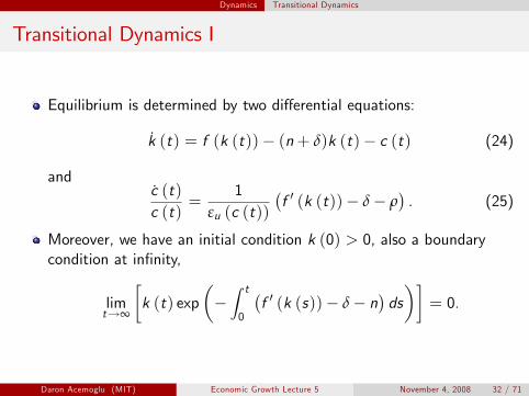
Equilibrium is determined by two di¤erential equations:
k (t) = f (k (t))� (n+ δ)k (t)� c (t) (24)
andc (t)c (t)
=1
εu (c (t))
�f 0 (k (t))� δ� ρ
�. (25)
Moreover, we have an initial condition k (0) > 0, also a boundarycondition at in�nity,
limt!∞
�k (t) exp
��Z t
0
�f 0 (k (s))� δ� n
�ds��
= 0.
Daron Acemoglu (MIT) Economic Growth Lecture 5 November 4, 2008 32 / 71

Dynamics Transitional Dynamics
Transitional Dynamics II
Appropriate notion of saddle-path stability:
consumption level (or equivalently µ) is the control variable, and c (0)(or µ (0)) is free: has to adjust to satisfy transversality conditionsince c (0) or µ (0) can jump to any value, need that there exists aone-dimensional manifold tending to the steady state (stable arm).If there were more than one path equilibrium would be indeterminate.
Economic forces are such that indeed there will be a one-dimensionalmanifold of stable solutions tending to the unique steady state.
See Figure.
Daron Acemoglu (MIT) Economic Growth Lecture 5 November 4, 2008 33 / 71
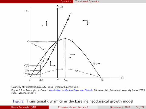
Dynamics Transitional Dynamics
c(t)
kgold0k(t)
k(0)
c’(0)
c’’(0)
c(t)=0
k(t)=0
k*
c(0)
c*
k
Figure: Transitional dynamics in the baseline neoclassical growth modelDaron Acemoglu (MIT) Economic Growth Lecture 5 November 4, 2008 34 / 71
Courtesy of Princeton University Press. Used with permission. Figure 8.1 in Acemoglu, K. Daron. Introduction to Modern Economic Growth. Princeton, NJ: Princeton University Press, 2009. ISBN: 9780691132921.
Dynamics Transitional Dynamics
Transitional Dynamics: Su¢ ciency
Why is the stable arm unique?Three di¤erent (complementary) lines of analysis
1 Su¢ ciency Theorem2 Global Stability Analysis3 Local Stability Analysis
Su¢ ciency Theorem: solution starting in c (0) and limiting to thesteady state satis�es the necessary and su¢ cient conditions, and thusunique solution to household problem and unique equilibrium.
Proposition In the neoclassical growth model described above, withAssumptions 1, 2, assumptions on utility above andAssumption 40, there exists a unique equilibrium pathstarting from any k (0) > 0 and converging to the uniquesteady-state (k�, c�) with k� given by (21). Moreover, ifk (0) < k�, then k (t) " k� and c (t) " c�, whereas ifk (0) > k�, then k (t) # k� and c (t) # c� .
Daron Acemoglu (MIT) Economic Growth Lecture 5 November 4, 2008 35 / 71

Dynamics Transitional Dynamics
Global Stability Analysis
Alternative argument:
if c (0) started below it, say c 00 (0), consumption would reach zero,thus capital would accumulate continuously until the maximum level ofcapital (reached with zero consumption) k > kgold . This would violatethe transversality condition. Can be established that transversalitycondition necessary in this case, thus such paths can be ruled out.if c (0) started above this stable arm, say at c 0 (0), the capital stockwould reach 0 in �nite time, while consumption would remain positive.But this would violate feasibility (a little care is necessary with thisargument, since necessary conditions do not apply at the boundary).
Daron Acemoglu (MIT) Economic Growth Lecture 5 November 4, 2008 36 / 71
Dynamics Transitional Dynamics
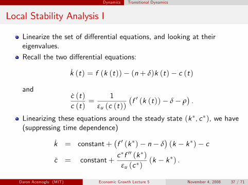
Local Stability Analysis I
Linearize the set of di¤erential equations, and looking at theireigenvalues.
Recall the two di¤erential equations:
k (t) = f (k (t))� (n+ δ)k (t)� c (t)
andc (t)c (t)
=1
εu (c (t))
�f 0 (k (t))� δ� ρ
�.
Linearizing these equations around the steady state (k�, c�), we have(suppressing time dependence)
k = constant+�f 0 (k�)� n� δ
�(k � k�)� c
c = constant+c�f 00 (k�)
εu (c�)(k � k�) .
Daron Acemoglu (MIT) Economic Growth Lecture 5 November 4, 2008 37 / 71

Dynamics Transitional Dynamics
Local Stability Analysis II
From (21), f 0 (k�)� δ = ρ, so the eigenvalues of this two-equationsystem are given by the values of ξ that solve the following quadraticform:
det
ρ� n� ξ �1c �f 00(k �)
εu (c �)0� ξ
!= 0.
Since c�f 00 (k�) /εu (c�) < 0, there are two real eigenvalues, onenegative and one positive.
Thus local analysis also leads to the same conclusion, but can onlyestablish local stability.
Daron Acemoglu (MIT) Economic Growth Lecture 5 November 4, 2008 38 / 71
Technological Change Technological Change
Technological Change and the Neoclassical Model
Extend the production function to:
Y (t) = F [K (t) ,A (t) L (t)] , (26)
whereA (t) = exp (gt)A (0) .
A consequence of Uzawa Theorem.: (26) imposes purelylabor-augmenting� Harrod-neutral� technological change.
Continue to adopt all usual assumptions, and Assumption 40 will bestrengthened further in order to ensure �nite discounted utility in thepresence of sustained economic growth.
Daron Acemoglu (MIT) Economic Growth Lecture 5 November 4, 2008 39 / 71
Technological Change Technological Change
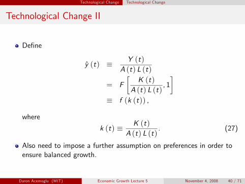
Technological Change II
De�ne
y (t) � Y (t)A (t) L (t)
= F�
K (t)A (t) L (t)
, 1�
� f (k (t)) ,
where
k (t) � K (t)A (t) L (t)
. (27)
Also need to impose a further assumption on preferences in order toensure balanced growth.
Daron Acemoglu (MIT) Economic Growth Lecture 5 November 4, 2008 40 / 71

Technological Change Technological Change
Technological Change III
De�ne balanced growth as a pattern of growth consistent with theKaldor facts of constant capital-output ratio and capital share innational income.
These two observations together also imply that the rental rate ofreturn on capital, R (t), has to be constant, which, from (8), impliesthat r (t) has to be constant.
Again refer to an equilibrium path that satis�es these conditions as abalanced growth path (BGP).
Balanced growth also requires that consumption and output grow at aconstant rate. Euler equation
c (t)c (t)
=1
εu (c (t))(r (t)� ρ) .
Daron Acemoglu (MIT) Economic Growth Lecture 5 November 4, 2008 41 / 71
Technological Change Technological Change
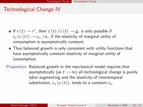
Technological Change IV
If r (t)! r �, then c (t) /c (t)! gc is only possible ifεu (c (t))! εu , i.e., if the elasticity of marginal utility ofconsumption is asymptotically constant.
Thus balanced growth is only consistent with utility functions thathave asymptotically constant elasticity of marginal utility ofconsumption.
Proposition Balanced growth in the neoclassical model requires thatasymptotically (as t ! ∞) all technological change is purelylabor augmenting and the elasticity of intertemporalsubstitution, εu (c (t)), tends to a constant εu .
Daron Acemoglu (MIT) Economic Growth Lecture 5 November 4, 2008 42 / 71

Technological Change Technological Change
Example: CRRA Utility I
Recall the Arrow-Pratt coe¢ cient of relative risk aversion for atwice-continuously di¤erentiable concave utility function U (c) is
R = �U00 (c) cU 0 (c)
.
Constant relative risk aversion (CRRA) utility function satis�es theproperty that R is constant.
Integrating both sides of the previous equation, setting R to aconstant, implies that the family of CRRA utility functions is given by
U (c) =
(c1�θ�11�θ if θ 6= 1 and θ � 0ln c if θ = 1
,
with the coe¢ cient of relative risk aversion given by θ.
Daron Acemoglu (MIT) Economic Growth Lecture 5 November 4, 2008 43 / 71

Technological Change Technological Change
Example: CRRA Utility II
With time separable utility functions, the inverse of the elasticity ofintertemporal substitution (de�ned in equation (16)) and thecoe¢ cient of relative risk aversion are identical.
Thus the family of CRRA utility functions are also those withconstant elasticity of intertemporal substitution.
Link this utility function to the Gorman preferences: consider aslightly di¤erent problem in which an individual has preferencesde�ned over the consumption of N commodities fc1, ..., cNg given by
U (fc1, ..., cNg) =(
∑Nj=1
c1�θj1�θ if θ 6= 1 and θ � 0
∑Nj=1 ln cj if θ = 1
. (28)
Daron Acemoglu (MIT) Economic Growth Lecture 5 November 4, 2008 44 / 71
Technological Change Technological Change
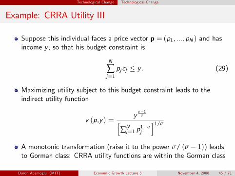
Example: CRRA Utility III
Suppose this individual faces a price vector p = (p1, ..., pN ) and hasincome y , so that his budget constraint is
N
∑j=1pjcj � y . (29)
Maximizing utility subject to this budget constraint leads to theindirect utility function
v (p,y) =y
σ�1σh
∑Nj=1 p
1�σj
i1/σ
A monotonic transformation (raise it to the power σ/ (σ� 1)) leadsto Gorman class: CRRA utility functions are within the Gorman class
Daron Acemoglu (MIT) Economic Growth Lecture 5 November 4, 2008 45 / 71

Technological Change Technological Change
Example: CRRA Utility IV
If all individuals have CRRA utility functions, then we can aggregatetheir preferences and represent them as if it belonged to a singleindividual.
Now consider a dynamic version of these preferences (de�ned overin�nite horizon):
U =
(∑∞t=0 βt
c (t)1�θ�11�θ if θ 6= 1 and θ � 0
∑∞t=0 βt ln c (t) if θ = 1
.
The important feature here is not that the coe¢ cient of relative riskaversion constant, but that the intertemporal elasticity of substitutionis constant.
Daron Acemoglu (MIT) Economic Growth Lecture 5 November 4, 2008 46 / 71

Technological Change Technological Change
Technological Change V
Given the restriction that balanced growth is only possible with aconstant elasticity of intertemporal substitution, start with
u (c (t)) =
(c (t)1�θ�11�θ if θ 6= 1 and θ � 0ln c(t) if θ = 1
,
Elasticity of marginal utility of consumption, εu , is given by θ.
When θ = 0, these represent linear preferences, when θ = 1, we havelog preferences, and as θ ! ∞, in�nitely risk-averse, and in�nitelyunwilling to substitute consumption over time.
Assume that the economy admits a representative household withCRRA preferencesZ ∞
0exp (�(ρ� n)t) c (t)
1�θ � 11� θ
dt, (30)
Daron Acemoglu (MIT) Economic Growth Lecture 5 November 4, 2008 47 / 71
Technological Change Technological Change
Technological Change VI
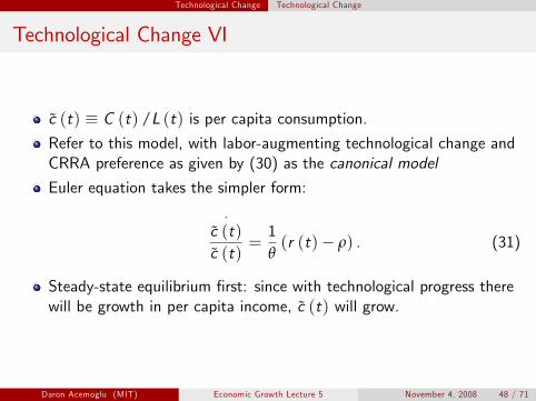
c (t) � C (t) /L (t) is per capita consumption.Refer to this model, with labor-augmenting technological change andCRRA preference as given by (30) as the canonical model
Euler equation takes the simpler form:
�c (t)c (t)
=1θ(r (t)� ρ) . (31)
Steady-state equilibrium �rst: since with technological progress therewill be growth in per capita income, c (t) will grow.
Daron Acemoglu (MIT) Economic Growth Lecture 5 November 4, 2008 48 / 71

Technological Change Technological Change
Technological Change VII
Instead de�ne
c (t) � C (t)A (t) L (t)
� c (t)A (t)
.
This normalized consumption level will remain constant along theBGP:
c (t)c (t)
��
c (t)c (t)
� g
=1θ(r (t)� ρ� θg) .
Daron Acemoglu (MIT) Economic Growth Lecture 5 November 4, 2008 49 / 71

Technological Change Technological Change
Technological Change VIII
For the accumulation of capital stock:
k (t) = f (k (t))� c (t)� (n+ g + δ) k (t) ,
where k (t) � K (t) /A (t) L (t).Transversality condition, in turn, can be expressed as
limt!∞
�k (t) exp
��Z t
0
�f 0 (k (s))� g � δ� n
�ds��
= 0. (32)
In addition, equilibrium r (t) is still given by (8), so
r (t) = f 0 (k (t))� δ
Daron Acemoglu (MIT) Economic Growth Lecture 5 November 4, 2008 50 / 71
Technological Change Technological Change
Technological Change IX
Since in steady state c (t) must remain constant:
r (t) = ρ+ θg
orf 0 (k�) = ρ+ δ+ θg , (33)
Pins down the steady-state value of the normalized capital ratio k�
uniquely.
Normalized consumption level is then given by
c� = f (k�)� (n+ g + δ) k�, (34)
Per capita consumption grows at the rate g .
Daron Acemoglu (MIT) Economic Growth Lecture 5 November 4, 2008 51 / 71

Technological Change Technological Change
Technological Change X
Because there is growth, to make sure that the transversalitycondition is in fact satis�ed substitute (33) into (32):
limt!∞
�k (t) exp
��Z t
0[ρ� (1� θ) g � n] ds
��= 0,
Can only hold if ρ� (1� θ) g � n > 0, or alternatively :Assumption 4:
ρ� n > (1� θ) g .
Remarks:
Strengthens Assumption 40 when θ < 1.Alternatively, recall in steady state r = ρ+ θg and the growth rate ofoutput is g + n.Therefore, equivalent to requiring that r > g + n.
Daron Acemoglu (MIT) Economic Growth Lecture 5 November 4, 2008 52 / 71

Technological Change Technological Change
Technological Change XI
Proposition Consider the neoclassical growth model with laboraugmenting technological progress at the rate g andpreferences given by (30). Suppose that Assumptions 1, 2,assumptions on utility above hold and ρ� n > (1� θ) g .Then there exists a unique balanced growth path with anormalized capital to e¤ective labor ratio of k�, given by(33), and output per capita and consumption per capitagrow at the rate g .
Steady-state capital-labor ratio no longer independent of preferences,depends on θ.
Positive growth in output per capita, and thus in consumption percapita.With upward-sloping consumption pro�le, willingness to substituteconsumption today for consumption tomorrow determinesaccumulation and thus equilibrium e¤ective capital-labor ratio.
Daron Acemoglu (MIT) Economic Growth Lecture 5 November 4, 2008 53 / 71

Technological Change Technological Change
c(t)
kgold0k(t)
k(0)
c’(0)
c’’(0)
c(t)=0
k(t)=0
k*
c(0)
c*
k
Figure: Transitional dynamics in the neoclassical growth model with technologicalchange.
Daron Acemoglu (MIT) Economic Growth Lecture 5 November 4, 2008 54 / 71
Courtesy of Princeton University Press. Used with permission. Figure 8.1 in Acemoglu, K. Daron. Introduction to Modern Economic Growth. Princeton, NJ: Princeton University Press, 2009.
ISBN: 9780691132921.
Technological Change Technological Change
Technological Change XII
Steady-state e¤ective capital-labor ratio, k�, is determinedendogenously, but steady-state growth rate of the economy is givenexogenously and equal to g .
Proposition Consider the neoclassical growth model with laboraugmenting technological progress at the rate g andpreferences given by (30). Suppose that Assumptions 1, 2,assumptions on utility above hold and ρ� n > (1� θ) g .Then there exists a unique equilibrium path of normalizedcapital and consumption, (k (t) , c (t)) converging to theunique steady-state (k�, c�) with k� given by (33).Moreover, if k (0) < k�, then k (t) " k� and c (t) " c�,whereas if k (0) > k�, then c (t) # k� and c (t) # c�.
Daron Acemoglu (MIT) Economic Growth Lecture 5 November 4, 2008 55 / 71
Technological Change Technological Change
Example: CRRA and Cobb-Douglas
Production function is given by F (K ,AL) = K α (AL)1�α, so that
f (k) = kα,
Thus r = αkα�1 � δ.
Suppressing time dependence, Euler equation:
cc=1θ
�αkα�1 � δ� ρ� θg
�,
Accumulation equation:
kk= kα�1 � δ� g � n� c
k.
De�ne z � c/k and x � kα�1, which implies thatx/x = (α� 1) k/k.
Daron Acemoglu (MIT) Economic Growth Lecture 5 November 4, 2008 56 / 71
Technological Change Technological Change
Example II
Therefore,xx= � (1� α) (x � δ� g � n� z) (35)
zz=cc� kk,
Thus
zz=
1θ(αx � δ� ρ� θg)� x + δ+ g + n+ z
=1θ((α� θ)x � (1� θ)δ+ θn)� ρ
θ+ z . (36)
Di¤erential equations (35) and (36) together with the initial conditionx (0) and the transversality condition completely determine thedynamics of the system.
Daron Acemoglu (MIT) Economic Growth Lecture 5 November 4, 2008 57 / 71

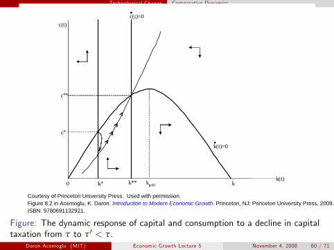
Technological Change Comparative Dynamics
Comparative Dynamics I
Comparative statics: changes in steady state in response to changesin parameters.
Comparative dynamics look at how the entire equilibrium path ofvariables changes in response to a change in policy or parameters.
Look at the e¤ect of a change in tax on capital (or discount rate ρ)
Consider the neoclassical growth in steady state (k�, c�).
Tax declines to τ0 < τ.
From Propositions above, after the change there exists a uniquesteady state equilibrium that is saddle path stable.
Let this steady state be denoted by (k��, c��).
Since τ0 < τ, k�� > k� while the equilibrium growth rate will remainunchanged.
Daron Acemoglu (MIT) Economic Growth Lecture 5 November 4, 2008 58 / 71

Technological Change Comparative Dynamics
Comparative Dynamics II
Figure: drawn assuming change is unanticipated and occurs at somedate T .
At T , curve corresponding to c/c = 0 shifts to the right and laws ofmotion represented by the phase diagram change.
Following the decline c� is above the stable arm of the new dynamicalsystem: consumption must drop immediately
Then consumption slowly increases along the stable arm
Overall level of normalized consumption will necessarily increase, sincethe intersection between the curve for c/c = 0 and for k/k = 0 willnecessarily be to the left side of kgold .
Daron Acemoglu (MIT) Economic Growth Lecture 5 November 4, 2008 59 / 71
Technological Change Comparative Dynamics
c(t)
kgold0k(t)
k*
c(t)=0
k(t)=0
k**
c**
c*
k
Figure: The dynamic response of capital and consumption to a decline in capitaltaxation from τ to τ0 < τ.
Daron Acemoglu (MIT) Economic Growth Lecture 5 November 4, 2008 60 / 71
Courtesy of Princeton University Press. Used with permission. Figure 8.2 in Acemoglu, K. Daron. Introduction to Modern Economic Growth. Princeton, NJ: Princeton University Press, 2009. ISBN: 9780691132921.

Policy and Quantitative Analysis The Role of Policy
The Role of Policy I
Growth of per capita consumption and output per worker (per capita)are determined exogenously.But level of income, depends on 1/θ, ρ, δ, n, and naturally the formof f (�).Proximate causes of di¤erences in income per capita: here explainthose di¤erences only in terms of preference and technologyparameters.Link between proximate and potential fundamental causes:
e.g. intertemporal elasticity of substitution and the discount rate canbe as related to cultural or geographic factors.
But an explanation for cross-country and over-time di¤erences ineconomic growth based on di¤erences or changes in preferences isunlikely to be satisfactory.More appealing: link incentives to accumulate physical capital (andhuman capital and technology) to the institutional environment.
Daron Acemoglu (MIT) Economic Growth Lecture 5 November 4, 2008 61 / 71

Policy and Quantitative Analysis The Role of Policy
The Role of Policy II
Simple way: through di¤erences in policies.
Introduce linear tax policy: returns on capital net of depreciation aretaxed at the rate τ and the proceeds of this are redistributed back tothe consumers.
Capital accumulation equation remains as above:
k (t) = f (k (t))� c (t)� (n+ g + δ) k (t) ,
But interest rate faced by households changes to:
r (t) = (1� τ)�f 0 (k (t))� δ
�,
Daron Acemoglu (MIT) Economic Growth Lecture 5 November 4, 2008 62 / 71
Policy and Quantitative Analysis The Role of Policy
The Role of Policy III
Growth rate of normalized consumption is then obtained from theconsumer Euler equation, (31):
c (t)c (t)
=1θ(r (t)� ρ� θg) .
=1θ
�(1� τ)
�f 0 (k (t))� δ
�� ρ� θg
�.
Identical argument to that before implies
f 0 (k�) = δ+ρ+ θg1� τ
. (37)
Higher τ, since f 0 (�) is decreasing, reduces k�.Higher taxes on capital have the e¤ect of depressing capitalaccumulation and reducing income per capita.But have not so far o¤ered a reason why some countries may taxcapital at a higher rate than others.
Daron Acemoglu (MIT) Economic Growth Lecture 5 November 4, 2008 63 / 71

A Quantitative Evaluation A Quantitative Evaluation
A Quantitative Evaluation I
Consider a world consisting of a collection J of closed neoclassicaleconomies (with the caveats of ignoring technological, trade and�nancial linkages across countriesEach country j 2 J admits a representative household with identicalpreferences, Z ∞
0exp (�ρt)
C 1�θj � 11� θ
dt. (38)
There is no population growth, so cj is both total or per capitaconsumption.Equation (38) imposes that all countries have the same discount rateρ.All countries also have access to the same production technologygiven by the Cobb-Douglas production function
Yj = K 1�αj (AHj )
α , (39)
Hj is the exogenously given stock of e¤ective labor (human capital).Daron Acemoglu (MIT) Economic Growth Lecture 5 November 4, 2008 64 / 71

A Quantitative Evaluation A Quantitative Evaluation
A Quantitative Evaluation II
The accumulation equation is
Kj = Ij � δKj .
The only di¤erence across countries is in the budget constraint for therepresentative household,
(1+ τj ) Ij + Cj � Yj , (40)
τj is the tax on investment: varies across countries because of policiesor di¤erences in institutions/property rights enforcement.
1+ τj is also the relative price of investment goods (relative toconsumption goods): one unit of consumption goods can only betransformed into 1/ (1+ τj ) units of investment goods.
The right-hand side variable of (40) is still Yj : assumes that τj Ij iswasted, rather than simply redistributed to some other agents.
Daron Acemoglu (MIT) Economic Growth Lecture 5 November 4, 2008 65 / 71

A Quantitative Evaluation A Quantitative Evaluation
A Quantitative Evaluation III
Without major consequence since CRRA preferences (38) can beexactly aggregated across individuals.
Competitive equilibrium: solution to maximization of (38) subject to(40) and the capital accumulation equation.
Euler equation of the representative household
CjCj=1θ
�(1� α)
(1+ τj )
�AHjKj
�α
� δ� ρ
�.
Steady state: because A is assumed to be constant, the steady statecorresponds to Cj/Cj = 0. Thus,
Kj =(1� α)1/α AHj
[(1+ τj ) (ρ+ δ)]1/α
Daron Acemoglu (MIT) Economic Growth Lecture 5 November 4, 2008 66 / 71
A Quantitative Evaluation A Quantitative Evaluation
A Quantitative Evaluation IV
Thus countries with higher taxes on investment will have a lowercapital stock, lower capital per worker, and lower capital output ratio(using (39) the capital output ratio is simply K/Y = (K/AH)α) insteady state.Substituting into (39), and comparing two countries with di¤erenttaxes (but the same human capital):
Y (τ)Y (τ0)
=
�1+ τ0
1+ τ
� 1�αα
(41)
So countries that tax investment at a higher rate will be poorer.Advantage relative to Solow growth model: extent to which di¤erenttypes of distortions will a¤ect income and capital accumulation isdetermined endogenously.A plausible value for α is 2/3, since this is the share of labor incomein national product.
Daron Acemoglu (MIT) Economic Growth Lecture 5 November 4, 2008 67 / 71
A Quantitative Evaluation A Quantitative Evaluation
A Quantitative Evaluation V
For di¤erences in τ�s across countries there is no obvious answer:
popular approach: obtain estimates of τ from the relative price ofinvestment goods (as compared to consumption goods)data from the Penn World tables suggest there is a large amount ofvariation in the relative price of investment goods.
E.g., countries with the highest relative price of investment goodshave relative prices almost eight times as high as countries with thelowest relative price.
Using α = 2/3, equation (41) implies:
Y (τ)Y (τ0)
� 81/2 � 3.
Thus, even very large di¤erences in taxes or distortions are unlikely toaccount for the large di¤erences in income per capita that we observe.
Daron Acemoglu (MIT) Economic Growth Lecture 5 November 4, 2008 68 / 71
A Quantitative Evaluation A Quantitative Evaluation
A Quantitative Evaluation VI
Parallels discussion of the Mankiw-Romer-Weil approach:
di¤erences in income per capita unlikely to be accounted for bydi¤erences in capital per worker alone.need sizable di¤erences in the e¢ ciency with which these factors areused, absent in this model.
But many economists have tried (and still try) to use versions of theneoclassical model to go further.
Motivation is simple: if instead of using α = 2/3, we take α = 1/3
Y (τ)Y (τ0)
� 82 � 64.
Thus if there is a way of increasing the responsiveness of capital orother factors to distortions, predicted di¤erences across countries canbe made much larger.
Daron Acemoglu (MIT) Economic Growth Lecture 5 November 4, 2008 69 / 71

A Quantitative Evaluation A Quantitative Evaluation
A Quantitative Evaluation VII
To have a model in which α = 1/3, must have additionalaccumulated factors, while still keeping the share of labor income innational product roughly around 2/3.
E.g., include human capital, but human capital di¤erences appear tobe insu¢ cient to explain much of the income per capita di¤erencesacross countries.
Or introduce other types of capital or perhaps technology thatresponds to distortions in the same way as capital.
Daron Acemoglu (MIT) Economic Growth Lecture 5 November 4, 2008 70 / 71

Conclusions
Conclusions
Major contribution: open the black box of capital accumulation byspecifying the preferences of consumers.
Also by specifying individual preferences we can explicitly compareequilibrium and optimal growth.
Paves the way for further analysis of capital accumulation, humancapital and endogenous technological progress.
Did our study of the neoclassical growth model generate new insightsabout the sources of cross-country income di¤erences and economicgrowth relative to the Solow growth model? Largely no.
This model, by itself, does not enable us to answer questions aboutthe fundamental causes of economic growth.
But it clari�es the nature of the economic decisions so that we are ina better position to ask such questions.
Daron Acemoglu (MIT) Economic Growth Lecture 5 November 4, 2008 71 / 71